Abstract
In this paper, we propose informed weighted non-negative matrix factorization (NMF) methods using an -divergence cost function. The available information comes from the exact knowledge/boundedness of some components of the factorization—which are used to structure the NMF parameterization—together with the row sum-to-one property of one matrix factor. In this contribution, we extend our previous work which partly involved some of these aspects to -divergence cost functions. We derive new update rules which are extendthe previous ones and take into account the available information. Experiments conducted for several operating conditions on realistic simulated mixtures of particulate matter sources show the relevance of these approaches. Results from a real dataset campaign are also presented and validated with expert knowledge.
1. Introduction
Source apportionment consists of estimating the particulate matter (PM) sources present in the ambient air together with their relative concentrations. A source is fully characterized by a profile which gathers the m chemical species’ proportions (expressed in ng/μg) that constitute it. Usually, several, say n, PM samples are collected using an automated sampler, then characterized to asses the chemical composition. Each of them can be written as a mixture of p profiles, with different concentrations (expressed in ng/m). Mathematically, if we respectively denote by X, G, and F as the non-negative data matrix, contribution matrix, and profile matrix, the collected data reads
While being known under the name of (blind) source separation in the signal/image processing community, Equation (1) is called the receptor model in the chemistry community. In practice, the latter should satisfy the following properties [1]:
- The entries of G and F are non-negative (one cannot assume a negative mass in G nor a negative proportion of chemical species in F).
- The product must fit the data matrix X.
- When one entry of the product does not fit the entry , we should then checki.e., the estimated mass of a chemical species in a sample should not be above the corresponding measured one.
As a consequence, estimating the unknown matrices G and F is mainly performed using positive matrix factorization (PMF) [2] and, in particular, using its popular version from the US Environmental Protection Agency.
Independently from the PMF investigations done by the chemistry community, Equation (1) has been massively considered by the signal/image processing and the machine learning communities which processed it with non-negative matrix factorization (NMF) techniques [3].
The general idea behind NMF is to minimize a discrepancy measure between X and the estimated product . Such a problem has been extensively studied in the past years. Historically—apart from pioneering work [4]—most methods are based on an alternating optimization of the factor matrices. NMF has been massively investigated because of the more interpretable results it provides when compared with methods without sign constraints. NMF was successfully applied to many fields, e.g., hyperspectral unmixing [5,6], astrophysics [7,8], fluorescence spectroscopy for agro-food analysis [9], audio signals [10], or environmental data processing [11].
It should be noticed that NMF is flexible and can take into consideration additional assumptions to provide a better estimation of the NMF factors. In the literature, assumptions such as sparseness [12,13], fixed row and/or column sums [13,14], structure in the matrix factors [15,16], or orthogonality constraints [17] were investigated.
Solving Equation (1) can be performed by appropriately choosing a discrepancy measure between X and . When this measure is the Frobenius norm of their difference, the possible presence of a few outliers may corrupt the NMF enhancement. As a consequence, robust NMF methods were proposed to deal with a predefined number of outliers. While some of them decompose the data matrix into the sum of a low-rank and a sparse matrix—where the latter contains the outlying component [18]—most ones consider some modified cost functions as dissimilarity measures which gave rise to flexible and robust algorithms, e.g., Bregman-NMF [19], -NMF [20], -NMF [21,22], -NMF [23], Correntropy-NMF [24], Huber-NMF [25] (it should be noticed that the Huber cost function has also been considered for robust PMF [26]).
Lastly, it should be noticed that in receptor models, each data point is provided with an uncertainty measure and PMF actually solves a weighted optimization problem [4,26]. Weighted extensions of NMF have been also considered, e.g., to enhance the factorization [27] or to deal with missing entries [28,29]. However, it is known than both the PMF [30] and the standard NMF techniques face some convergence issues (however, the convergence of NMF is guaranteed under some separability assumptions [3] which are not satisfied in practice in the considered application and which are thus out of the scope of this paper) [3].
As a consequence, we investigated the enhancement provided by informed NMF. In Ref. [31], the use of a Gaussian plume model enables us to assess the presence or absence of some punctual sources, depending on wind measures, and source and sensor locations which allowed us to fix some entries of G to zero. In the absence of a punctual source, such an information should be dropped. In Ref. [32], an informed NMF-based weighted criterion takes into consideration the known values of some terms of F (Informed NMF has also been proposed in [33] where the known entries are seen as a penalization term in the NMF optimization problem) in order to improve the separation. For that purpose, we introduced a specific parameterization for NMF methods using a Frobenius norm. This approach should be considered as a flexible NMF counterpart of [34] in between blind source separation—where no information on F is provided—and regression, where F is fully known. While it was shown in practice to be less sensitive than blind NMF to convergence issues, this method can still be affected by outliers which are present in many receptor modeling problems.
In this paper, we thus extend our previous work [32] by (i) investigating and discussing several -divergence expressions, (ii) exploring different data normalization procedures combined with set values (as profiles are chemical species proportions, the rows of F are normalized), and (iii) adding minimum and maximum bounds to some of the unknown values of F. The methods we propose in this paper have been partially introduced in [35,36], in the framework of the -divergence only. We generalize here [35,36] to the -divergence and we provide a detailed study of their performance, shown on both realistic simulations and real data campaign.
The remainder of the paper is structured as follows. We recall some properties of the -divergence in Section 2. Section 3 introduces our proposed NMF parameterization—which puts on light the special structure of the profile matrix in the NMF algorithm—while Section 4 is dedicated to the problem formulation. We introduce our proposed methods in Section 5 that we test in Section 6. Lastly, we conclude about the proposed work in Section 7. Appendix A introduces update rules for an alternative informed -NMF method.
2. Robust Cost Functions
2.1. Introduction to Modified Cost Functions
Chemical data often face some particular measures whose characteristics substantially differ from those which are commonly observed. From a signal processing point of view, such data may be considered as outliers which may degrade the performance of classical algorithms using the Frobenius norm in their cost function. Such an issue is often addressed in the field of robustness where the challenge is to design new algorithms which take into account the above corrupted data.
Apart from the low-rank plus sparse decomposition [18], robust NMF algorithms using modified cost functions were investigated. Indeed, these robust functions provide less penalization to large entries of the residual matrix, which is defined as
Among them, the Huber cost function accounts for the differentiable connection between the and norms, according to the residual value with respect to an adaptive cutoff parameter. Another popular modified cost function stands for the correntropy measure [24] which accounts for a bounded and non-convex discrepancy measure.
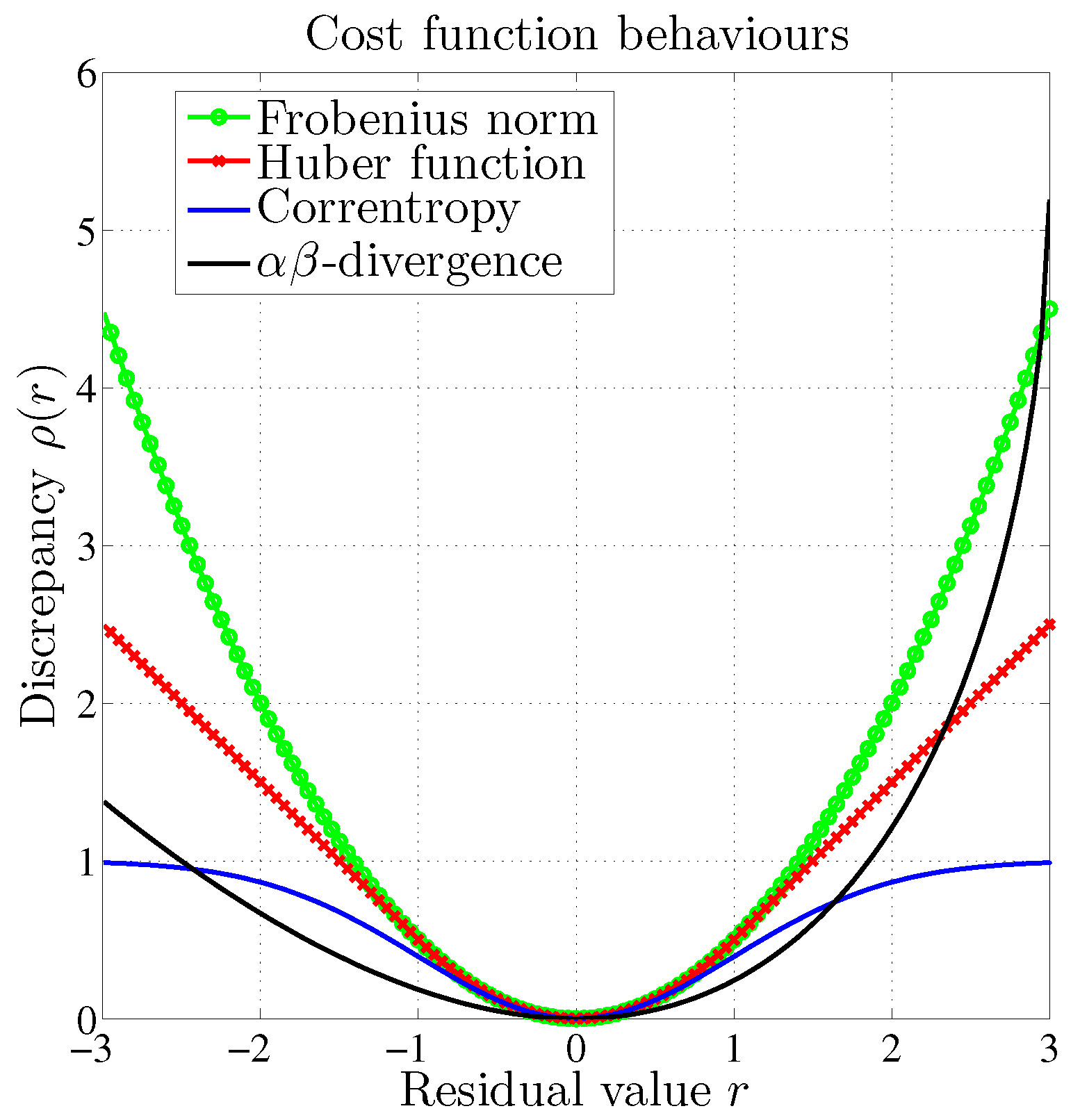
In contrast with the above measures, the -divergence is not a norm as it is not symmetrical. Figure 1 shows an example of the behavior of such functions which are penalizing the values of the residual in different ways. As mentioned earlier, the -divergence is the only cost function to present a possible asymmetric behavior around the null residual value. Hopke [1] highlighted the need for methods dedicated to chemical source apportionment which enforce a positive residual value. This situation fits well with the configuration described in Figure 1.

Figure 1.
Behavior of several dissimilarity measures with respect to the residual value.
2.2. -Divergence
The -divergence (For special values of , the reader is invited to consult [23]) is a parametric discrepancy measure which may be used to evaluate the gap between two scalar quantities p and q, i.e., ,
Special values of the parameters lead to very famous divergence measures [23], such as -divergences or -divergences [21]. These divergences are different from classical norms in the sense that they check some common properties—e.g., non-negativity—while others such as symmetry, scalability and triangular inequality are not satisfied.
Cichocki et al. [23] study the influence of the parameters and on the robustness of the estimated data (they also establish general connections between the general -divergence and the scaled -order -divergence with an zoom of its arguments). To this aim, they express the sensitivity to outliers by computing the differentiation with respect to an unknown parameter here replaced for simplicity with an entry of F, namely , i.e.,
where
and
For the sake of comparison, sensitivity equations of M-estimators [37] are usually designed for the weighted Frobenius cost function (corresponding to and in a -divergence), i.e.,
where accounts for the general entry of the weight matrix. This weight is usually viewed as a confidence index into the corresponding data. As a consequence, a large residual together with a large weight leads to large modifications in the estimates. In the frame of Equation (8), the weight entry reads
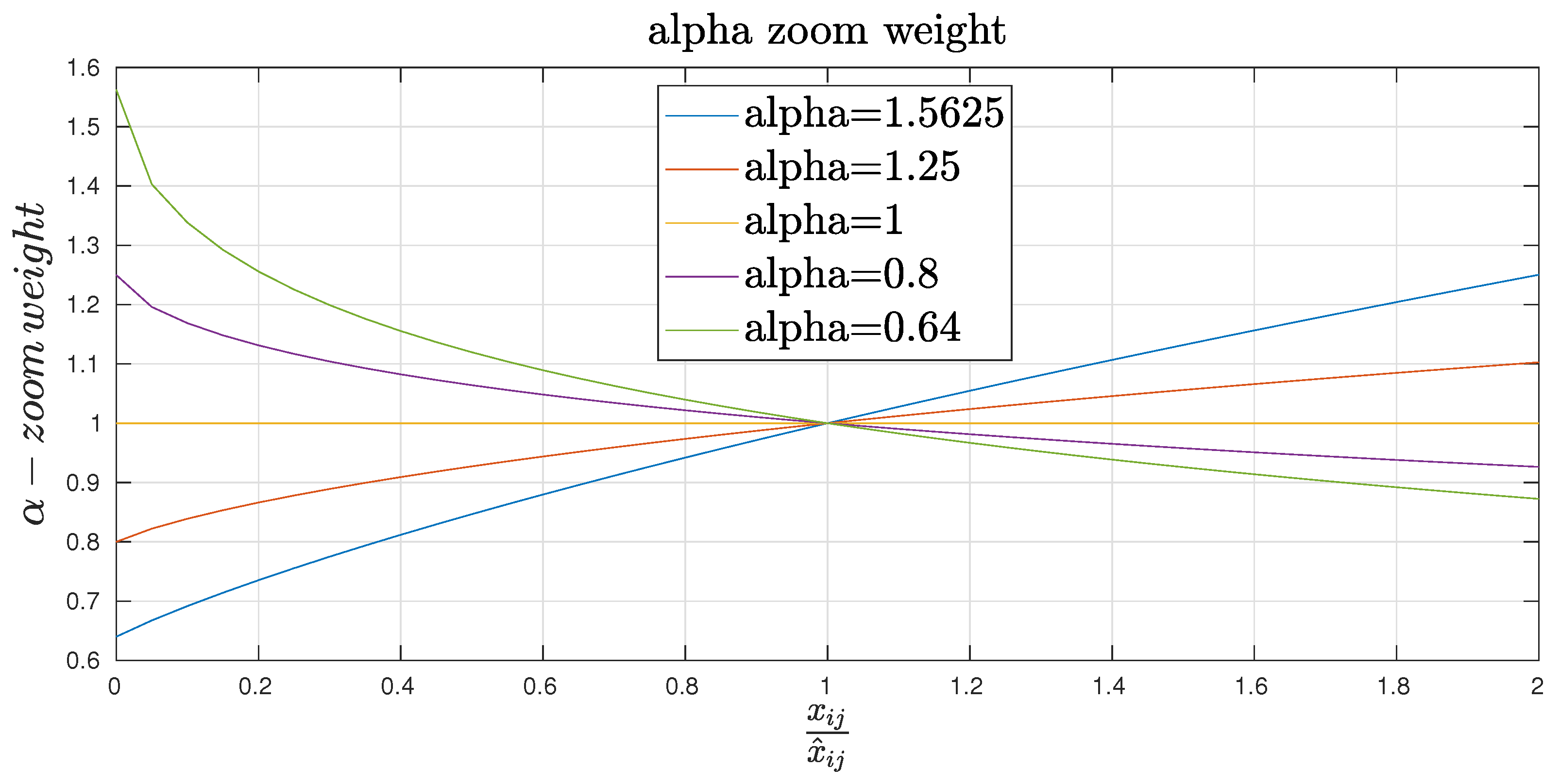
Figure 2 describes the -zoom weight as a function of the ratio for different values of . It turns out that provides small weight to large values of the ratio . In other words, this situation does not induce big changes in the estimates. Outliers such as will be allowed in this context.
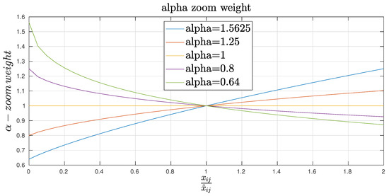
Figure 2.
The -zoom weight.
Equation (8) combines two effects, namely an -zoom and an weight effect. When , the emphasis of the -zoom is put on larger values of the ratio while the emphasis is put on smaller values of this ratio when . These properties are recalled in Table 1. The weight effect in is expressed as a function of in Table 2.

Table 1.
Properties of -zoom.

Table 2.
Weighting effect on the -divergence.
To summarize, can be used to control the influence of large or small ratios in the estimator through the -zoom, while provides some control on the weighting of the ratios depending on the demand to better fit to larger or smaller values of the model [23]. Gathering these properties, the space of values may be partitioned in several areas as described in Figure 3.
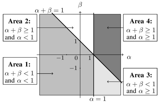
Figure 3.
Different areas as a function of and .
Each zone allows a certain kind of outliers. Areas 1 and 2 allow outliers of the form for large and small amplitudes of , respectively. Areas 3 and 4 accept outliers such as for large and small amplitudes of , respectively. Areas 1 and 3 favor a better fit to small values of X while areas 2 and 4 favor a better fit to large ones. As a consequence, for our considered application, we propose to favor a best fit for major species with respect to minor species. This leads to considering the case . Secondly, if the estimation does not fit the data, we prefer keeping situations where holds, as explained in Section 1 and in [1]. This fact results in the choice . These two conditions give rise to an area of interest which is area 2 and which is kept along the article (for convexity reasons in NMF [23], area 2 should be delimited to ).
2.3. Existing NMF Methods with Parametric Divergences
NMF methods are formulated as the global minimization of a cost function under the non-negativity of both factors G and F. Aside from pioneering work [4], NMF is classically performed through an iterative procedure which alternatively minimizes—for a fixed F (respectively G)—a discrepancy between X and . Multiplicative update rules were firstly proposed in [38] for the Frobenius norm and the Kullback–Leibler divergence. While being easy to implement, multiplicative algorithms only ensure that the cost function does not increase within iterations, which is not sufficient for getting a limit point. The study of NMF convergence through the Karush–Kuhn Tucker (KKT) conditions was explored by Lin [39]; stationarity is only a necessary condition of a local minimum. Moreover, some limit points which are not stationary may exist, especially if some components of F and G are initialized to zero.
Moreover, most algorithms are sensitive to the initialization and to the presence of outliers. Parametric divergences may reduce the influence of this last drawback by an appropriate choice of the hyperparameters.
Cichocki et al. [20] proposed multiplicative update rules with -divergence. The developed rules were based on the majorization-minimization (MM) strategy [40] but they may also be obtained in a heuristic way by using the KKT conditions or partial derivatives of the cost function as well.
Févotte and Idier [21] proposed to use the -divergence as a cost function and derived different kinds of rules according to three different strategies involving the heuristic approach, the majorization-minimization strategy [40] and a new one called majorization-equalization. This last strategy provides a larger step size and a faster convergence. Hennequin et al. stated that the -divergence could be viewed as a special case of Bregman divergence [41], thus leading us to apply Bregman divergence theorems to -divergence. Cichocki et al. [23] proposed NMF based on generalized -divergences in the framework of majorization-minimization (MM).
Extending the work in [27,42] from the one hand and in [23] from the other hand, we introduced in [35] a weighted -NMF (-WNMF) defined for . It is straightforward to extend it to a Weighted -NMF which amounts to minimizing a weighted -divergence,
and yields
where
and
and respectively denote the componentwise product and division between two matrices. W is a weight matrix used to model the uncertainties associated to the data samples , and whose general element is set to . This approach encompasses several other methods, especially -NMF [23] if , i.e., for any i and j, , and -NMF [21] if additionally .
Apart from multiplicative updates, NMF based on alternating direction method of multipliers (ADMM) were recently proposed [43] for their ability to perform distributed computations for large scale data and in particular, Sun and Févotte introduced an approach based on the -divergence [22] while Zhu and Honeine [24] proposed a correntropy-based approach for large deviations. Such fast approaches are not required for the considered chemical application where the global computation time is not an issue.
3. Constraint Parameterization
In this paper, we assume the values of some components of the profile matrix F to be provided or bounded by experts. We thus propose a formalism which takes into account this knowledge. It extends our previous parameterization [32] which only considered equality constraints.
Let and be two binary matrices which inform the presence/absence of equality and inequality constraints on each element of the matrix F, respectively, i.e.,
We then define the binary matrices and as and , where is the matrix of ones. By construction, we obtain
We denote by the sparse matrix of set values, i.e.,
Please note that —the -th element of —is equal to zero when . We can easily prove that
Similarly, we define and the sparse matrices of upper and lower bounds (equality constraints could be considered as inequalities, with the same upper and lower bounds. However, in some preliminary tests, we found our proposed approaches to outperform those using bound constraints only), respectively, i.e.,
Let and be the i-th column of F and , respectively. A column may be expressed as
where and are respectively the vector of free parameters and the orthonormal basis of free parameters [32]. From Equation (20), we define as
and as the matrix gathering each column , i.e.,
4. General Problem Formulation
The proposed informed NMF methods consist of estimating the matrices G and F in order to get an approximate factorization (1) under the above constraints, i.e.,
where the weighted divergence is defined in Equation (11). The first constraint ensures that some predefined components of F are set while the second one forces the selected components to be bound-constrained. The last condition enforces each row of F to be normalized, i.e., , (Please note that the normalization met in remote sensing [44]—where the sum of each row of F is equal to one—is not similar, except in a noiseless case in the framework of exact factorization. Moreover, the normalization also differs from the one met in mobile sensor calibration [13] as the normalization is approximately satisfied in the latter).
The main challenge in the Equation (25) consists of finding solutions which are satisfying all the above constraints. The first constraint leads to consider the parametrization (23) that we used in [32]. By substituting the parametrization (23), Equation (25) becomes a constrained NMF with respect to G and , i.e.,
In the case of bound constraints only, no dedicated parameterization exists, but projective methods have been developed [45]. The row sum-to-one constraint has been taken under account by using a special parameterization in [14]. However, dealing with all the constraints together at the same time is a difficult task. We thus propose a less elegant, yet efficient strategy which consists of considering them sequentially. By dropping the bound constraint, we obtain the following reduced problem:
As an alternative to the above problem, please note that by combining Equations (1) and (23), we obtain
We can thus derive a slightly different problem, i.e.,
which yieldsslightly different update rules. We proposed in [35] some multiplicative update rules to solve Equation (29) in the case of -divergence only. The extension to the -divergence is derived in Appendix A.
As explained above, instead of looking for the solution of Equation (26) directly, we sequentially consider each additional set of information, i.e., we first estimate and F that we then normalize and project onto the set of admissible solutions (or that we project and then normalize, respectively) within iterations.
5. Proposed Informed -NMF Methods
5.1. Weighted -NMF with Set Constraints
In this section, we firstly aim to solve Equation (27) without the sum-to-one constraint. The whole strategy follows the majoration-minimization technique [40] and consists of (i) finding a majoring function which is convex with respect to the unknown parameters, and (ii) minimizing this auxiliary function instead of the original one.
Proposition 1.
Update rules for the free part of the profile matrix are
where (denoting ), we define
Proof.
We consider a column of the data since the divergence may be split into independent partial divergences. Using the notations defined in Section 3, we hereafter drop the index i for the vectors , , , and for the matrix . Let k be the current iteration index and let us define
The weighted -divergence between two corresponding column vectors reads
where ,
Provided that and noticing that is convex for and [23], Jensen’s inequality may be applied twice, i.e.,
and
where the superscript k is the current iteration number and is the j-th element of the free parameter vector introduced in Equation (20). Equation (34) together with expressions (36) and (37) yield the following auxiliary function:
Canceling its gradient leads to the optimum, i.e.,
which reads in its vector form
By combining Equation (21) with the above relationship, we derive the expression of one column of the matrix :
By replacing U according to Equation (32), and by noticing that , it results in the new update rule:
where
Similarly to [35], we derive the update rules by writing the matrix form of Equation (43), which completes the proof. □
Appendix A proposes the update rules for the problem (29). These rules are almost similar to those introduced above as they present some differences in the multiplicative mask. We show in Appendix A that the update rules proposed in the main part of this paper extend the ones proposed in Appendix A by iteratively updating the weights.
Update rules for G correspondto an unconstrained -WNMF driven by Equation (12) since no information is available on G. Their validity is only guaranteed within the convex domain, i.e., for . Outside this domain, some additional assumptions on the reconstructed data are needed to ensure the local convexity property [23]. As we chose to set and so that they belong to area 2 in Figure 3, the convexity domain reduces the possible area to the intersection between area 2 and the half-plane .
5.2. Normalization Procedures
In the considered application, the rows of the profile matrix are summed to one. This case is different from the one encountered in hyperspectral unmixing [44]—since our constraint cannot be split into independent vectorial subproblems—and in mobile sensor calibration [13] as the sum-constraint is only approximately satisfied in the latter. As a consequence, in our previous work [32,35], we used to normalize the matrices G and F in each iteration, after estimating them. We reformulate these steps below (see Section 5.2.1) while we investigate an alternative normalization procedure in Section 5.2.2. They are introduced in the framework of the above approach but the rules may be applied to our previous work [32,35] as well.
5.2.1. Classical Normalization
Let us define as the normalized profile matrix and the corresponding scaled contribution matrix. In order to hold the sum-to-one property, Lantéri et al. [14] proposed a change of variables under the form (please note that the normalization constraint can also be solved as a penalization term in the NMF problem formulation [13]. This setting is interesting when the sum constraint is approximately satisfied, which is not the case for the considered application).
which may be written under matrix form as
This equation enables to normalize the rows of F whereas the symmetric version enables to scale the columns of G correspondingly, i.e.,
The product then reads
which results in the expression of its general entry:
This means that the matrix product is maintained throughout the normalization process. Since the cost function to minimize only depends on this product, this property ensures the same decrease as in the unconstrained case within iterations.
The normalized expression of F—denoted —at iteration then reads
where
and where stands for the free part of the normalized matrix defined by . Noticing that
we express Equation (49) with respect to :
Similarly, we derive the update rules for , i.e.,
where —defined in Equation (14)—is computed with the unnormalized matrix which reads
Equations (52) and (53) thus provide the update rules for our first normalized and constrained WNMF method denoted -N-constrained and weighted NMF (CWNMF) below. Although the set profiles are lost within iterations due to the normalization process, we noticed in preliminary tests that they were recovered asymptotically.
5.2.2. Alternative Normalization
As an alternative, we now propose a second normalization which keeps the set constraints on F within iterations. Starting with Equation (30) that we normalize, it turns out that
where accounts for the matrix involving the sum of the free components for each source, and the other part of the expression represents the different proportions within the free profiles. Using the property (51), alternative update rules may be derived
This normalization keeps the constraints verified within iterations but may move along directions different from the steepest descent direction. During this process, the contribution matrix does not require a scale factor as in the first method since the scale factor is only applied to the free parameters of F. We then estimate using the unconstrained rules defined in Equations (12) and (14). The update rules (12) and (56) are associated with our second normalized and constrained WNMF method denoted -N-CWNMF below.
5.2.3. Description of Algorithm Acronyms
We proposed above some update rules for two methods for normalized and constrained WNMF. However, we also proposed different update rules in Appendix A for which the above normalizations can be applied. As these methods minimize the divergence between and the Residual , we add a “-R” to their acronym. Table 3 outlines the necessary information for each method. The pseudo code for -N-CWNMF(-R) methods is shown in Algorithm 1.

Table 3.
Our different non-negative matrix factorization (NMF) methods with normalization.
| Algorithm 1-N-constrained weighted non-negative matrix factorization (CWNMF) residual (-R) method. |
| while do Update F at fixed G according to Equation (52) or (56) Update G at fixed F according to Equation (12) or (53) end while |
5.3. Bound-Constrained Normalized and Weighted -NMF
We now focus on problem (25) which involves several kinds of constraints which should coexist simultaneously. To our knowledge, only Lin [45] deals with bound constraints and proposes to adapt the stepsize of projected gradient techniques in order to both decrease the cost function while holding the constraints. However, the work was devoted to bound constraints only, and his solution does not suit our problem with normalization.
As explained above, we propose to tackle them by applying a projection onto the admissible domain. Bound constraints act as safety barriers which prevent unrealistic solutions. However, the combination of normalization and projection should be applied in a predefined order. We thus propose below two structures:
- the bound constraint projection followed by a normalization stage,
- or the normalization followed by the projection.
5.3.1. Informed NMF with Bound Constraints and Normalization
In this subsection, we consider update rules for N-CWNMF methods. The same kind of procedure should be done for N-CWNMF approaches proposed above. We assume that we get at iteration k a normalized matrix and an unscaled (indeed, no scaling is applied on G in N-CWNMF, as explained in Section 5.2.2) contribution matrix . Combining Equations (24) and (54) provide
which may be simplified by using Equation (51), i.e.,
Applying the bound constraint then consists of
where is the projection operator defined by
The second normalization proposed in Section 5.2.2 consists of scaling the free part without changing the set components, which reads
This rule keeps the sum-to-one constraint and the set values. The bound constraints may be lost within because of the normalization but were found to be asymptotically recovered in our tests. The associated updates for G follows the unconstrained ones and it has not to be corrected by a scale factor, i.e.,
where has been introduced in Equation (14). The rules (61) and (62)—associated to our informed NMF approach named -BN-CWNMF—do not ensure the cancellation of the gradient of Equation (38) along iterations but they preserve two set of constraints among the three ones. Let us recall that the approach using the first proposed normalization—denoted -BN-CWNMF—can be derived with the same strategy. The pseudo code for -BN-CWNMF method is shown in Algorithm 2.
| Algorithm 2-BN-CWNMF method |
| while do Update F at fixed G according to Equation (61) Update G at fixed F according to Equation (62) end while |
5.3.2. Informed NMF with Normalization and Bound Constraints
The same procedure as above should be applied in the reverse order so that bound projection is applied as the last step of an iteration. When applied to Equation (58), the second normalization provides
The projection stage then leads to the unnormalized profile
Equations (62) and (64) account for the update rules in this last method, denoted as -NB-CWNMF. The pseudo code for NB-CWNMF method is shown in Algorithm 3.
| Algorithm 3-NB-CWNMF method |
| while do Update F at fixed G according to Equation (64) Update G at fixed F according to Equation (62) end while |
Please notice that only set and bound constraints are checked within iterations. Convergence towards a limit point ensures that limit matrices keep all the desired properties. As explained above, the same procedure with our first considered normalization may be applied, thus yielding an approach named -NB-CWNMF.
6. Experimental Results
In this section, the enhancement provided by our methods are investigated in both simulations and a real data campaign. In these tests, we aim to identify the sources (by their chemical profile) contributing to the total atmospheric suspended PM as well as to quantify their contribution. In both the simulations and the real dataset, we consider atmospheric particles with diameter equal to or below 10 μm (PM). In practice, these particles are trapped in a filter which is changed every 24 h. Each filter is then analyzed by chemists who derive the masses of several chemical species of interest for the considered application, i.e., for evaluating the impact of marine traffic on air pollution in a port city. Species under study are divided into 16 metal tracers—i.e., , , , , P, , , , V, , , , , , , and —8 water soluble ionic species—i.e., , , , , , , , and —carbon compounds—either organic (OC) or elementary (EC)—levoglucosan, and polyols.
In all these experiments, except when we tested the influence of these parameters, we set the values of and to 0.6 and 0.9, respectively. Indeed, such a couple of value lies in the recommended area 2 defined in Figure 3. Moreover, we found in preliminary tests that these values of and provided a better performance. As a consequence, we do not make them vary in the remainder of this section.
Moreover, the signal-to-noise ratio (SNR) enabled us to evaluate the data set and is defined as:
where and stand for the -th non-noisy data and the individual noise. This index is widely used in the literature [46].
6.1. Realistic Simulations
From the validated profile and contribution matrices obtained during the real campaign [47], simulation data were built by taking into account the individual uncertainty provided by the real campaign. In these simulations, the data matrix X thus consisted of a matrix—which correspond to the chemical composition (28 species) of 278 PM samples—associated with individual uncertainties, which are those provided by the chemical analysis.
In addition, we also considered several cases with outliers. It is assumed that outliers come from an additional positive individual contamination.
The mathematical model of the outliers was driven by a random vector including the locations of the outliers in the data matrix. For these locations, a multiplicative model was used depending of the trial number i (between 1 and 400).
where (resp. X) accounts for the with outliers noiseless data (resp. the without outliers noiseless data). The variable is a parameter which may be tuned in order to get a SNR after outliers ranging from 15 dB to 70 dB. In our tests, the outlier deviation increased with the trial number i. In other words, for low trial number, the multiplicative factor remained close to 1 in order to keep large. The effect of such outliers essentially depends on the location of the outliers. Indeed, if an outlier acts on a large entry of the data matrix, its impact on the SNR will be greater.
Then, a noise has to mimic the chemical measurement process. The chemical measurement process only gives a concentration value together with an uncertainty. So, every value within this interval is equally possible. A uniform noise which is designed on a limited support was proposed. This support may be truncated on the left side if the uncertainty is greater than the corresponding data.
Among the 278 samples, 10 and 20 outliers were considered. Practically, we noticed that the signal-to-noise ratio (SNR) index then dropped in the worst case by 4 dB if the set of 20 outliers is taken into consideration with respect to the no outlier case.
6.1.1. Source Profiles
In this study, 10 sources are highlighted. Among them, some of them are purely natural or purely anthropogenic but some of them became anthropised. Table 4 describes major species present in each source profile. Other species than those listed in the corresponding source profile may be considered as negligible. Please note that—as we here consider simulations—the real profile matrix is perfectly known and is provided in Table A1. Also, one should notice that each source profile is presented under a per mil notation, i.e., it sums to a thousand instead of 1 and the only difference is a scale factor equal to 1000.

Table 4.
Features of the different source profiles.
6.1.2. Equality Constraints
Equality constraints or set values enable to inform the algorithm about some entries of the profile matrix. This knowledge is taken into account by specifying matrices and . These matrices are available in Appendix B. It is to be stressed that the only used knowledge here is the absence of some compounds in some source profiles. As a result, matrix reduced to . Then, it follows that our informed methods with residuals were identical to those without residual. As a consequence, we do not test the latter in the simulations below.
6.1.3. Initialization
An approximate prior knowledge of F was used as a starting point for each informed NMF algorithm. Table A3 gathers the different entries used. Then, a weighted quadratic estimation of the initial contribution matrix G [31] was performed so that each method has the same initial factors.
6.1.4. Performance Evaluation
Several performance indexes are available in the literature. However in this work, only the mixing-error ratio () index [52] is considered (please note that while specifically designed for measuring the estimation accuracy of a mixing matrix, the MER may also be used as a signal-to-inteference ratio (SIR) when applied to the profile matrix, and more specifically to ). It was computed over each column of G. For each source, a scalar quantity for source j expressed in may be obtained.
For one exact vector and its estimate , it is possible to write under the form
where and are respectively colinear and orthogonal to the exact vector . This decomposition allows to express the of source j, denoted as , defined as,
Infinite values mean exact separation while 0 correspond to an angle equal to . These values may be summed up into a vector which gathers the performance of each source. Generally, a global indicator is obtained by averaging each index over all sources, i.e.,
In all the cases under study, the MER (the results and the Matlab interpretation codes are already available at http://www-lisic.univ-littoral.fr/~delmaire/recherche.html) index [52] was represented as a function of the input SNR. In this study, intensive computations were performed with ten thousand iterations for each method over 400 tests. In our comparison, we dropped the PMF method as it is only available as a user interface (see https://www.epa.gov/air-research/positive-matrix-factorization-model-environmental-data-analyses) which prevents to compute several tests in a single command. Moreover, even for a single test, our expertise shows that PMF requires the uncertainties to be increased in order to perform a computation, but it did not make sense in this case. As a consequence, nine methods were selected and tested: among them, three are uninformed, two account for our informed methods with set values while the four remaining ones are our informed methods with bounds.
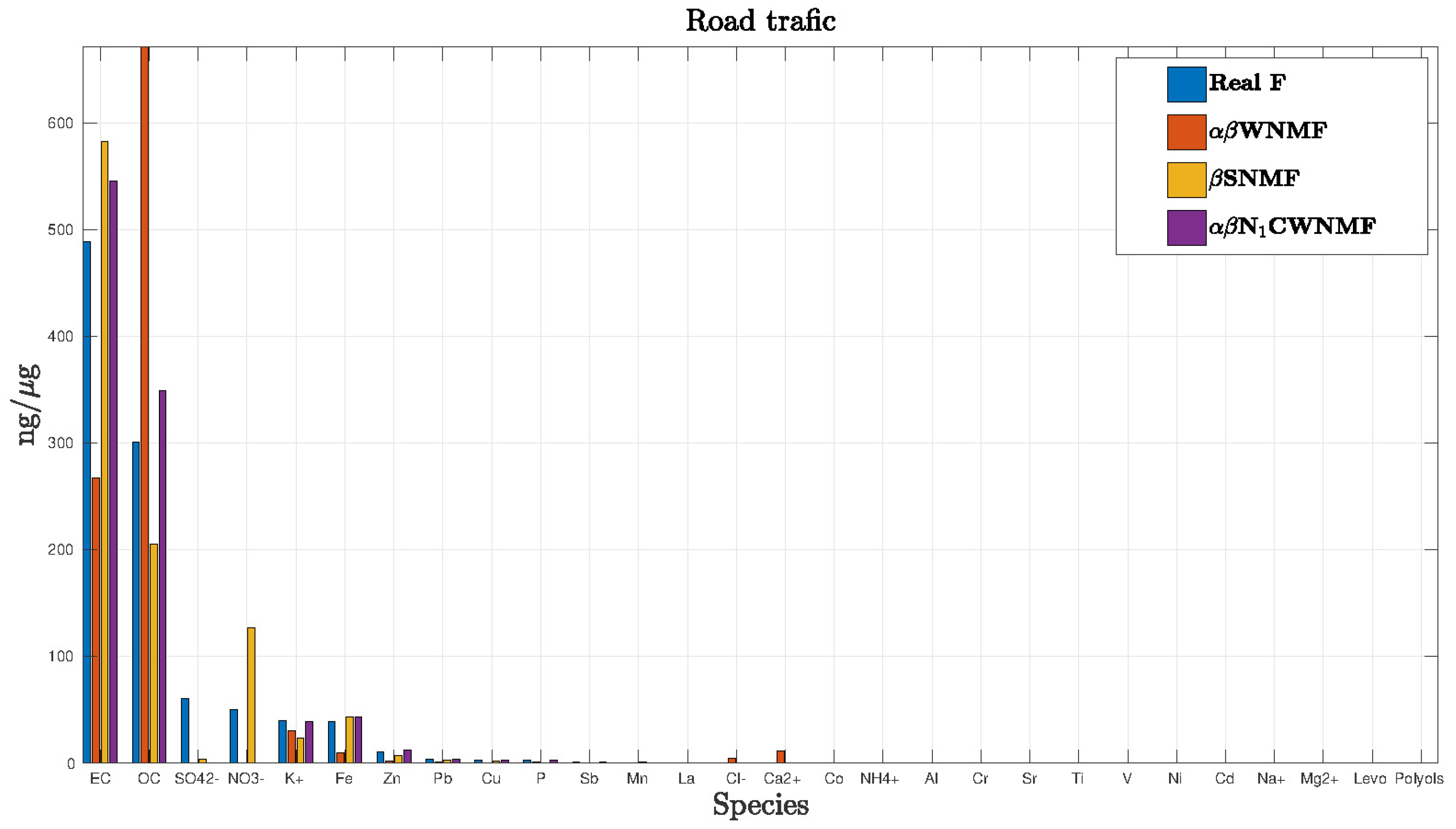
In order to get an idea, we chose to display the road traffic profile estimation in the case when input is equal to 24 dB (Figure 4). Species were represented in descending order of the real profile. We could notice that for this source, NCWNMF appears better than other methods.

Figure 4.
Estimation of the road traffic profile.
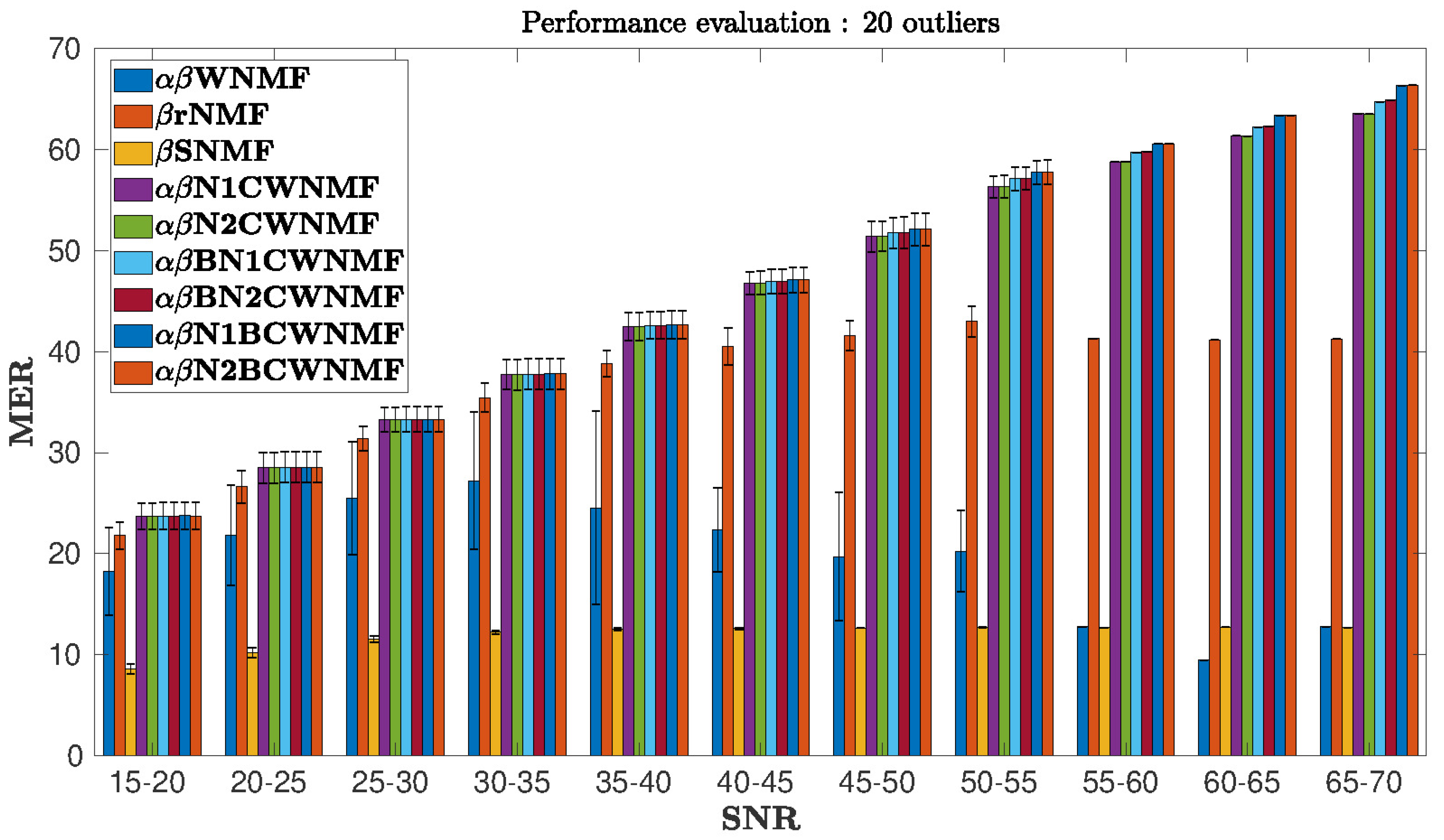
In our tests, the input SNR ranges from 15 to 70 dB. We decided to display only the performance of the methods for 20 outliers as shown in Figure 5 since the other tests provide similar results. The statistical performance is provided in Figure 5 by specifying the standard deviation in each slice of SNR and for each method.
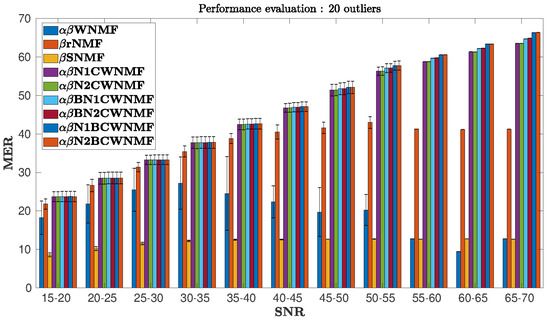
Figure 5.
MER vs. input signal-to-noise ratio (SNR). The case with 20 outliers.
Let us first analyze the enhancement provided by the non-informed NMF methods. One notice that the robust -WNMF [23] performs very poorly in all cases. Its standard deviation appears very large for a wide range of SNRs. Besides, RNMF—which stands for a robust NMF method [18]—behaves correctly for low SNRs while its performance decreases surprisingly for large SNRs. Moreover, we experimented a sparse NMF (SNMF) method [53] including a -divergence cost function together with L sparsity of one factor. We select one trial and test the performance for the parameter ranging from 0 to 2. The optimal value has been selected over 400 trials for the case of 20 outliers. SNMF provides inconsistent solutions in every slice of SNR.
We analyzed the performance of our proposed informed methods. Let us firstly focus on both informed methods with set values which were experimented, i.e., the -N1CWNMF and -N2CWNMF methods. Their performance appeared to be very similar in all the simulations. In practice, their MER was approximately equal to the SNR in every input SNR slice, which was expected according to our experience in preliminary tests.
The four informed NMF methods with bound constraints behaved similarly, except in a few slices where the SNR is large. Indeed, in low SNR, they are slightly better than -N1CWNMF (the gap is not visible due to the scale), but they outperform all the other tested methods as soon as the SNR becomes greater than 40 dB. The low gap in low SNR is essentially due to the fact that we inform F while the performance index is measured on G. In noisy tests—i.e., for a low SNR—the estimated matrix G does not benefit from the additional information on F, because of the important noise in X. However, we noticed an improvement on F for these tests, even if we cannot safely measure it, as the profiles might be correlated.
On the contrary, for medium and large SNR, the MER enhancement was significant for every bound-constrained informed NMF method. More precisely, -N1BCWNMF and -N2BCWNMF outperformed all the other methods with a significant gap as soon as the SNR increased.
We also explored in the synthetic example the use of a large range of and parameters within area 2 such that and . We noticed that the MER index for WNMF method was very sensitive to the choice of the parameters and also to the trial number. A successful tuning of these parameters was somehow difficult.
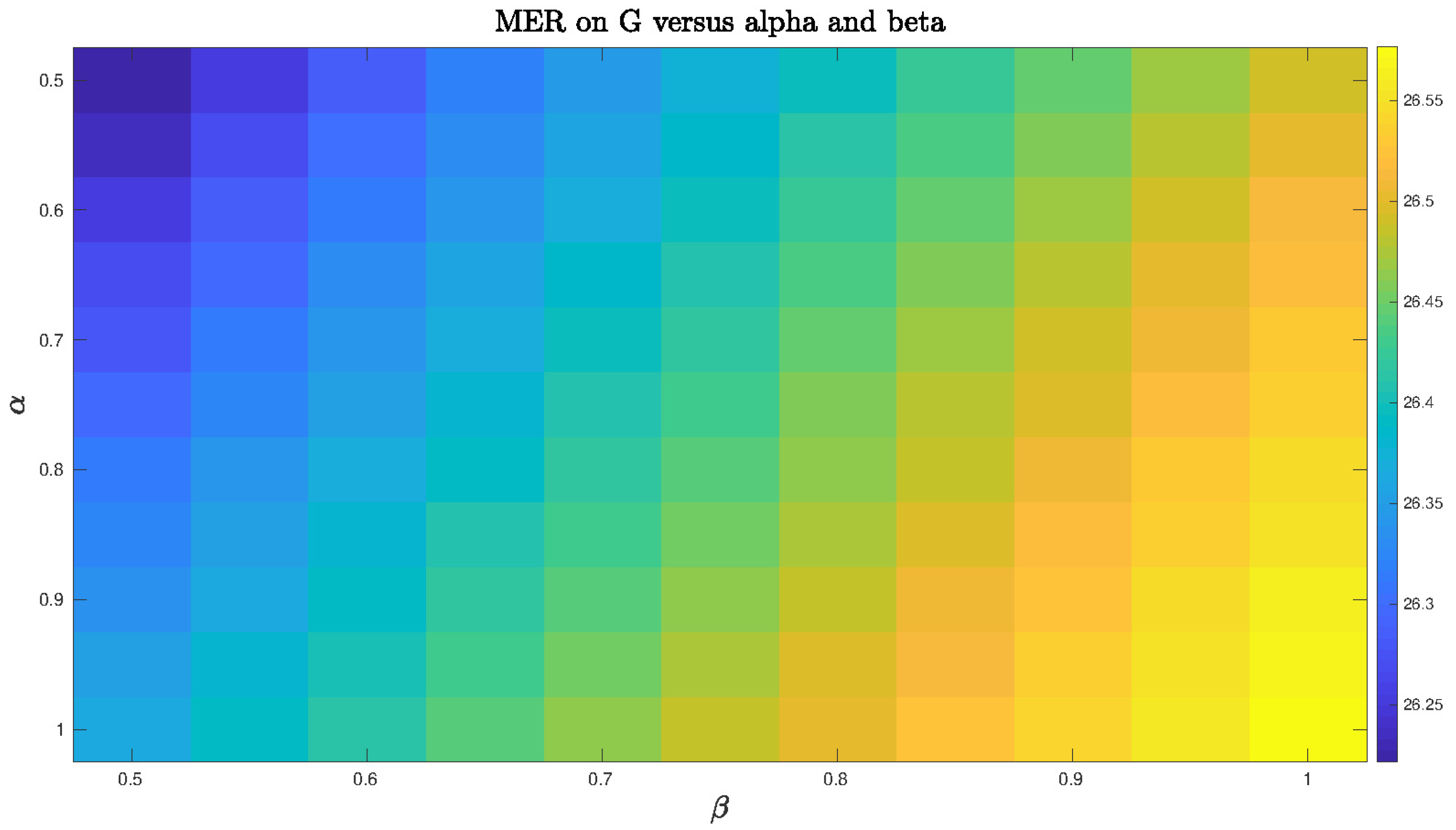
On the other hand, we experiment the same operating conditions for NCWNMF. We observe in Figure 6 that results are more stable than for the uninformed one. In this case, the choice of appears quite insensitive but the method remains satisfactory.

Figure 6.
Mixing-error ratio (MER) index for N constrained and weighted NMF mixing-error ratio (CWNMF) vs. and .
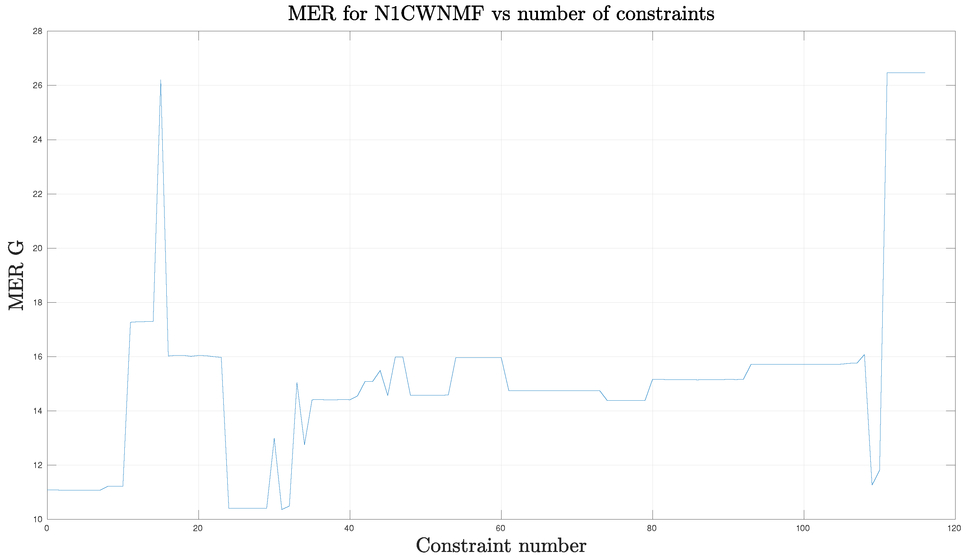
In addition, we could wonder how constraints affect the results. First, we potentially may use 117 set values and roughly 60 bound constraints. We decided to inspect the influence of dropping set values only. For that purpose, we progressively turned on one set value at a time for each column and according to the increasing order of the row index, until the 117 constraints were reached. We plot the MER performance according to the number of constraints in Figure 7.
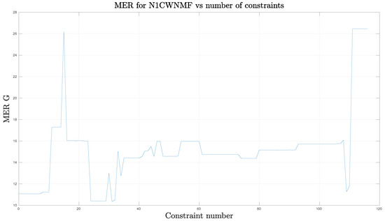
Figure 7.
MER versus constraint number. The case with 20 outliers.
Contrary to what should be expected, adding constraints may sometimes degrade the performance suddenly or conversely. There seems to be set of constraints which fit better to the situation. This conclusion is quite surprising and the design of appropriate constraints seems an open question.
To conclude, these methods provide a good performance in every situation and are thus better-suited for the considered application.
6.2. Real Data Case
The real data campaign was conducted by Dr C. Roche during her Ph.D. thesis [54], within the UCEIV laboratory (Université du Littoral Côte d’Opale). The first goal of this thesis was to study how much the shipping traffic in the English Channel, one of the most important in the world, can contribute to the atmospheric PM concentration in coastal area, such as the Hauts–de–France region. In her work, some characteristic species of maritime traffic emissions have been evidenced. Then, some flexible bound profiles and set profile entries were proposed. Using this knowledge, the challenge was to implement an informed NMF method—as those developed in [32]—in order to reconstruct the PM origin.
Contrary to [54], we here would like to drop some of the bound information and to test whether or not the new methods that we propose in this paper are still competitive.
6.2.1. Context
A sampling campaign has been conducted using a Digitel DA80 sampler over a long period—i.e., 16 months—in Cape Gris–Nez and over a shorter period—i.e., three months—in the port of Calais, which enabled us to get 278 sample measurements. Cape Gris–Nez and Calais are two coastal sites in the eastern part of the English channel. The first one is a rural site whereas the port of Calais is the second busiest in passenger traffic in Europe with 10.8 million of passengers and over 80 arrivals and departures of ferries per day in average in 2014 [55].
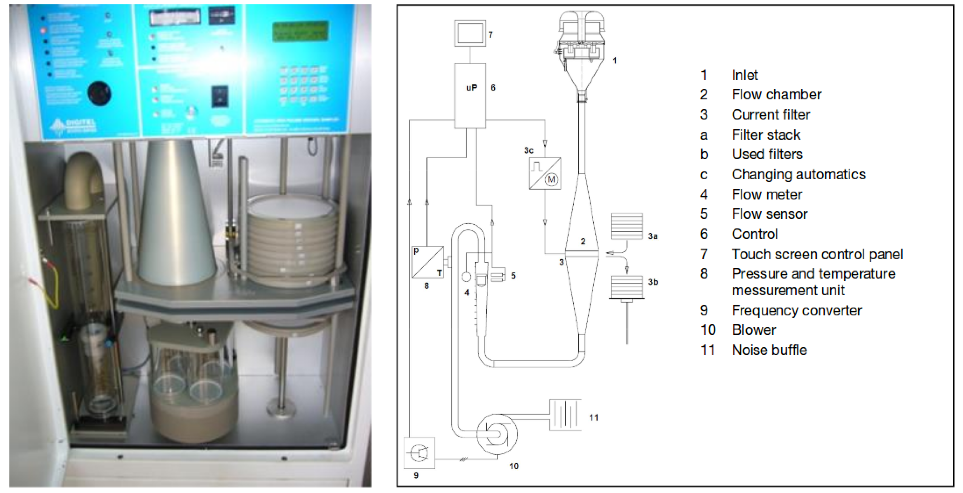
The DA80 device (see Figure 8) is an equipment which is able to trap PM on filters, which are stored and a posteriori analyzed for chemical composition. A special sieve enabled us to select only PM, i.e., PM whose diameter was lower than m. The machine is also able to save wind conditions and time. The sampling period was chosen equal to 24 h. Along this period, meteorological conditions concentration levels were highly varying. Thus, after analyzing the filters, several data files were available to address the pollution source apportionment problem.
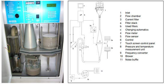
Figure 8.
Digitel DA80 high volume sampler used for data acquisition (source of the right plot: Digitel).
6.2.2. Input Data
Appendix C provides operating conditions for the run which are performed. Based on the expert knowledge provided by chemists and on the information described in Table 4, a matrix —which defines 55 set value locations (among 278 profile entries)—is provided in Table A5. In the same way as in Section 6.1, the matrix is equal to . In addition, the initial profile matrix is chosen by an expert and is provided in Appendix C.
6.2.3. Results Evaluation
The results were obtained in the case of 10 identified sources and iterations for each method. The profiles under study are specified in Table 4. However, their estimation remains a difficult task for several reasons which listed hereafter:
- Data are corrupted by an unknown number of outliers. Their origin may be of various kinds, e.g., the presence of a new source which affects the data at some sparse moments.
- Data are very noisy. In particular, an additional overall pollution—whose level highly varies over time—can not be assigned to a particular source and can significantly decrease the overall SNR.
- Some source profiles may be geometrically close, only a few tracer species are able to distinguish them.
Even if a database with source profiles is available at http://source-apportionment.jrc.ec.europa.eu/Specieurope/sources.aspx, a universal profile for a given source does not exist. When comparing our result, they all appear highly consistent with the published one in the Specieurope database. We display the source profiles in a descending order of expected species (MPMPthis task was designed by the chemist co-authors of the paper). A correct source profile was then displayed as decreasing proportions from the left to the right of each figure. On the contrary, a large proportion on the right part of a profile plot implies that the estimation has partly failed.
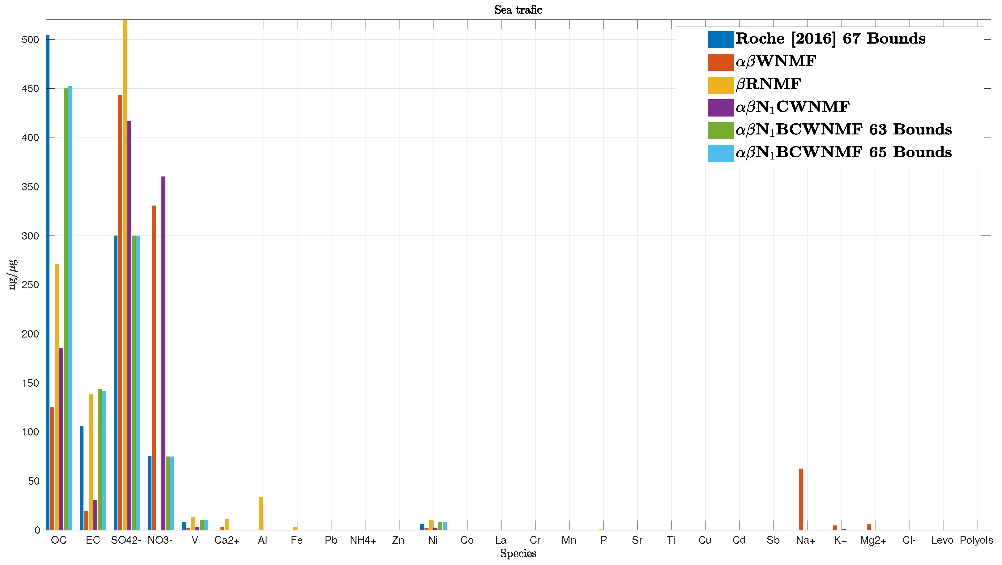
Among the 10 source profiles, some of them are well recovered. We only show in Figure 9 the estimated sea traffic source profile as it is difficult to recover. As mentioned above, it is expected that proportions are decreasing from the left to the right side of the figure. The order has been built based on ship profiles from the European database and from the literature [50,51,54]. To process these data, we compare the enhancement provided by two non-informed methods, i.e., the -WNMF and the -RNMF [18] and three informed methods, i.e., the method used in [54] and our methods -N1CWNMF, and its bound-constrained extension -N1BCWNMF. Other bound methods were dropped since they turn out in Section 6.1 to behave roughly similar to -N1BCWNMF. Note that Roche [54] used 67 constraints while we only use 63 and 65 bound constraints in the tested bound-constrained informed -NMF method, respectively.
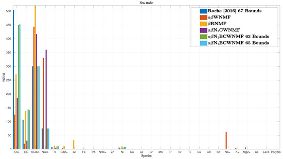
Figure 9.
Estimation of the sea traffic source profile.
It may be noticed that blind NMF methods, i.e., the -WNMF and the -RNMF, and our -N1CWNMF method are overestimating and species while underestimating OC and EC compounds. The estimated sea traffic profile thus appears not to be very realistic with these methods. Besides, bound-constrained WNMF methods behave similarly and report good estimations for major species. However, these estimations reach the proposed bounds for , , and species among the 28 species under study. For example, is limited by the maximum value provided in Table A4. Finally, these bound-constrained NMF methods outperform all the other methods for the sea traffic re-construction.
Using the estimation provided by each method, it is possible to reconstruct each species’ concentration, and especially the V and compounds since they are tracers of the sea traffic activity [54]. In other words, the V and species can only be found in the sea traffic source. Moreover, the ratio V over is often assimilated to a value between 2 and 3 [51], and is found to be between 1.2 to 1.5 for the three bound-constrained WNMF methods, which is close to the expected ratio.
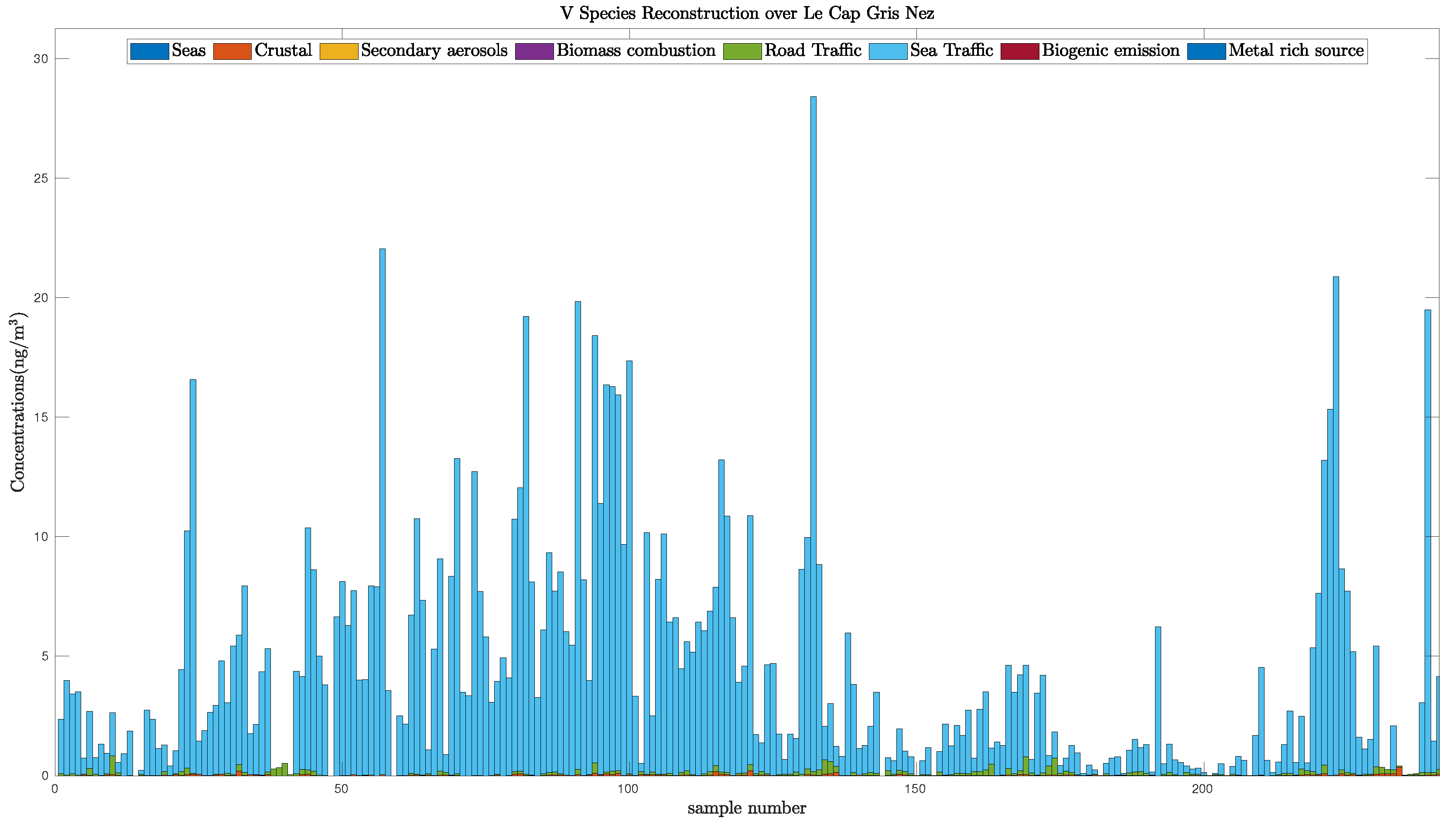
To confirm this fact, we plot the reconstruction of the V species in Figure 10. This shows that this compounds is mainly due to Sea Traffic. More than 98 per cent of the V species originates from the sea traffic source which is consistent with the chemist’s expectations.

Figure 10.
V species reconstruction over Cape Gris–Nez.
7. Conclusions
In this paper, we tackled an informed non-negative matrix factorization problem where the profile matrix lives in a specific subspace. We proposed several informed NMF methods combining -divergence and a specific structure of one matrix factor provided by the considered problem. This work extends our previous informed NMF [32]—assuming some values of one of the factor matrices to be known—by considering generalized divergences, and by leading to alternative update rules and normalization. The update rules may be viewed as projective multiplicative updates applied to a special structure of the profile matrix. The relevance of these extensions were shown on realistic simulations of natural and industrial PM source apportionment—with various input SNR conditions and various numbers of outliers—and on a real data case. In practice, these informed methods are more robust than blind NMF, and provide results which are consistent with the chemical expert, even in the presence several outliers. In future work, we will investigate new soft constraints to inform NMF and alternatives to multiplicative updates.
Author Contributions
Conceptualization, G.D., M.P., A.L., and G.R.; methodology, G.D., M.O., and A.L.; software, G.D., M.O., and A.L.; validation, G.D., M.O., M.P., G.R., F.L., and D.C.; formal analysis, G.D. and M.O.; investigation, G.D. and M.O.; resources, F.L. and D.C.; data curation, G.D., M.O., F.L., and D.C.; writing—original draft preparation, G.D. and M.P.; visualization, G.D. and M.O., supervision, G.R. and D.C.; project administration, G.R. and D.C.; funding acquisition, G.D., G.R., F.L., and D.C.
Funding
This research was funded partly by the integrated steel and mining company ArcelorMittal, and partly by the DREAL Nord-Pas-de-Calais agency within the ECUME project.
Acknowledgments
The experiments presented in this paper were carried out using the CALCULCO computing platform, supported by SCoSI/ULCO.
Conflicts of Interest
The authors declare no conflict of interest. The funding sponsors had no role in the design of the study; in the collection, analyses, or interpretation of data; in the writing of the manuscript, and in the decision to publish the results.
Abbreviations
The following abbreviations are used in this manuscript:
| CWNMF | Constrained and weighted NMF |
| KKT | Karush–Kuhn Tucker |
| EC | Elementary carbon |
| MER | Mixing-error ratio |
| MM | Majorization-minimization |
| NMF | Non-negative matrix factorization |
| OC | Organic carbon |
| PM | Particulate matter |
| RNMF | Robust NMF |
| SIR | Signal-to-interference ratio |
| SNR | Signal-to-noise ratio |
| WNMF | Weighted NMF |
Appendix A. Update Rules for Problem (29)
In this appendix, we aim to develop update rules for problem (29), for which we drop the sum-to-one constraint. The structure of the proof follows the same steps as in Section 5.1 within a MM strategy.
Proposition A1.
Update rules for the free part of the profile matrix are
where
Proof.
We focus on a column of the data and drop hereafter the index i for the vectors , , , and for the matrix . Let us define the residual vector as
Combining Equations (21) and (32) leads to
where U is defined in Equation (32), and where has been defined in Equation (35).
Using the convexity of for and [23], Jensen inequality may be applied once, resulting in:
where the superscript k is the current iteration number and is the j-th element of the free parameters vector introduced in (20). Equation (A4) together with Equation (A5) yield the majoring function
Cancelling its gradient leads to
which reads in vector form:
By combining the definition (21) with the above relationship, we derive the expression of one column of the matrix .
By replacing U according to Equation (32), and by noticing that , it results in the new update rule:
where accounts for
As explained in Section 5.1, it should be noticed the update rules for both variants of the weighted -divergence cost function provide almost similar update rules. In fact, in Equation (31) and in Equation (A2) are the same if we replace W in the latter expression by
As G is updated at each NMF iteration, the value of W in Equation (A14) varies at each iteration, which means that the update rules proposed in the main part of this paper extend the one proposed in Appendix A by iteratively updating the weights.
Appendix B. Operating Conditions for the Simulations
Table A1 specifies the different entries of the true profile matrix for simulations.
Prior information is provided through the specification of both and . We choose to select only set values which specify the absence of some species in the profile matrix. As a consequence, is equal to . The position of these known zero entries are provided in Table A2.
The chemists are able to provide an initial profile matrix which is given in Table A3. It is to be noted that the same initial matrix is applied for both the informed and non informed methods. It should be noticed that the known zeros in F are initialized as 1.00 .

Table A1.
Theoretical source profile used in the simulations.
Table A1.
Theoretical source profile used in the simulations.
| Profiles | Al | Cr | Fe | Mn | P | Sr | Ti | Zn | V | Ni | Co | Cu | Cd | Sb |
|---|---|---|---|---|---|---|---|---|---|---|---|---|---|---|
| Sea | 0.0019 | 0 | 0 | 0 | 2.5 | 0.2034 | 0 | 0 | 0 | 0 | 0 | 0 | 0 | 0 |
| Aged sea | 0 | 7.2351 | 0 | 0 | 0.5 | 0.4 | 1.877 | 0 | 0 | 0 | 1.785 | 1.7941 | 0 | 0 |
| Crustal | 119.13 | 8.589 | 77.35 | 1.782 | 3.0680 | 0.7846 | 8.9121 | 1.868 | 0.3503 | 0 | 0.0276 | 0.0081 | 0 | 0 |
| nitrates | 4.00 | 2 | 3.5 | 0.11 | 0.0749 | 0 | 0 | 0.7742 | 0 | 0 | 7.0408 | 0.1 | 6.486 | 0.01975 |
| sulfate | 0 | 5 | 0 | 0.02825 | 0.05313 | 0 | 0 | 0.1334 | 0 | 0 | 0.003287 | 8.00 | 0 | 0 |
| Biomass | 0.001 | 0 | 2.554 | 0.05527 | 0 | 1.016 | 0 | 0.1415 | 0 | 0 | 0 | 0 | 0 | 0.0385 |
| Road traffic | 0 | 0 | 39.0414 | 0.1404 | 2.659 | 0 | 0 | 10.908 | 0 | 0 | 1.00 | 2.7712 | 0 | 0.8964 |
| Sea traffic | 0.001147 | 1.2012 | 0.1002 | 0 | 0 | 0.0217 | 9.42 | 0 | 7.4920 | 5.5348 | 0.1829 | 1.752 | 1.315 | 0 |
| Biogenic | 0 | 0 | 0 | 0 | 14.528 | 0.04308 | 8.941 | 0 | 0 | 0 | 0 | 0 | 0 | 5.2 |
| Metal | 64.430 | 33.332 | 780.16 | 33 | 0.7 | 2 | 0 | 0 | 0 | 10 | 0.15 | 1.5 | 1.55 | 0 |
| Bis | OC | EC | Levo. | Polyols | ||||||||||
| Sea | 0 | 0 | 297.03 | 0 | 10.71 | 32.75 | 9.183 | 581.02 | 0 | 69.08 | 0 | 0 | 0 | 0 |
| Aged sea | 0 | 0.1 | 280 | 0 | 4 | 30 | 10 | 1.00 | 395 | 150 | 30 | 0 | 0 | 0 |
| Crustal | 0.0594 | 0 | 1.8333 | 4.36 | 5 | 5 | 301.81 | 0 | 49.95 | 39.96 | 384.92 | 0 | 0 | 0 |
| nitrates | 7.178 | 0.2075 | 0 | 216.26 | 3.2 | 0 | 0 | 1.21 | 730.73 | 0 | 45 | 0 | 0 | 9.027 |
| sulfate | 0 | 0.0729 | 0 | 260.83 | 4.43 | 0 | 0 | 8.66 | 0 | 680.59 | 53.84 | 0 | 0 | 0 |
| Biomass | 0 | 0.1007 | 2.650 | 2.85 | 12.26 | 0.001 | 11.67 | 25.48 | 35.16 | 56.84 | 692.10 | 91.14 | 69.78 | 1.477 |
| Road traffic | 0.0121 | 3.353 | 0 | 5.14 | 39.84 | 0 | 3.00 | 3.40 | 50.19 | 60.22 | 301.13 | 488.81 | 0 | 0 |
| Sea traffic | 0.0941 | 0 | 0 | 0.0626 | 0 | 0 | 0 | 0 | 75.17 | 300.69 | 500.76 | 109.87 | 0 | 0 |
| Biogenic | 0 | 0 | 5.023 | 0.0968 | 29.056 | 0 | 0 | 0.2975 | 0 | 20.094 | 854.02 | 0 | 0 | 76.83 |
| Metal | 0.2215 | 22.95 | 0 | 0 | 0 | 0 | 0 | 0 | 0 | 50.00 | 0 | 0 | 0 | 0 |

Table A2.
Matrix used in the simulations.
Table A2.
Matrix used in the simulations.
| Al | Cr | Fe | Mn | P | Sr | Ti | Zn | V | Ni | Co | Cu | Cd | Sb | |
|---|---|---|---|---|---|---|---|---|---|---|---|---|---|---|
| Sea | 0 | 1 | 1 | 1 | 0 | 0 | 1 | 1 | 1 | 1 | 1 | 1 | 1 | 1 |
| Aged sea | 1 | 0 | 1 | 1 | 0 | 0 | 0 | 1 | 1 | 1 | 0 | 0 | 1 | 1 |
| Crustal | 0 | 0 | 0 | 0 | 0 | 0 | 0 | 0 | 0 | 1 | 0 | 0 | 1 | 1 |
| nitrates | 0 | 0 | 0 | 0 | 0 | 1 | 1 | 0 | 1 | 1 | 0 | 0 | 0 | 0 |
| sulfate | 1 | 0 | 1 | 0 | 0 | 1 | 1 | 0 | 1 | 1 | 0 | 0 | 1 | 1 |
| Biomass | 0 | 1 | 0 | 0 | 1 | 0 | 1 | 0 | 1 | 1 | 1 | 1 | 1 | 0 |
| Road traffic | 1 | 1 | 0 | 0 | 0 | 1 | 1 | 0 | 1 | 1 | 0 | 0 | 1 | 0 |
| Sea traffic | 0 | 0 | 0 | 1 | 1 | 0 | 0 | 1 | 0 | 0 | 0 | 0 | 0 | 1 |
| Biogenic | 1 | 1 | 1 | 1 | 0 | 0 | 0 | 1 | 1 | 1 | 1 | 1 | 1 | 0 |
| Metal | 0 | 0 | 0 | 0 | 0 | 0 | 1 | 1 | 1 | 0 | 0 | 0 | 0 | 1 |
| La | Pb | Na | NH | K | Mg | Ca | Cl | NO | SO | OC | EC | Levo. | Polyols | |
| Sea | 1 | 1 | 0 | 1 | 0 | 0 | 0 | 0 | 1 | 0 | 1 | 0 | 1 | 1 |
| Aged sea | 1 | 0 | 0 | 1 | 0 | 0 | 0 | 0 | 0 | 0 | 0 | 1 | 1 | 1 |
| Crustal | 0 | 0 | 0 | 0 | 0 | 0 | 0 | 1 | 0 | 0 | 0 | 1 | 1 | 1 |
| nitrates | 0 | 0 | 1 | 0 | 0 | 0 | 1 | 0 | 0 | 1 | 0 | 0 | 1 | 0 |
| sulfate | 1 | 0 | 1 | 0 | 0 | 0 | 1 | 0 | 1 | 0 | 0 | 0 | 1 | 1 |
| Biomass | 1 | 0 | 0 | 0 | 0 | 0 | 0 | 0 | 0 | 0 | 0 | 0 | 0 | 0 |
| Road traffic | 0 | 0 | 1 | 0 | 0 | 1 | 0 | 0 | 0 | 0 | 0 | 0 | 1 | 1 |
| Sea traffic | 0 | 0 | 1 | 0 | 1 | 0 | 1 | 0 | 0 | 0 | 0 | 0 | 1 | 1 |
| Biogenic | 1 | 1 | 0 | 0 | 0 | 0 | 1 | 0 | 0 | 0 | 0 | 1 | 1 | 0 |
| Metal | 0 | 0 | 1 | 0 | 1 | 0 | 1 | 1 | 1 | 0 | 1 | 1 | 1 | 1 |

Table A3.
Matrix used in the simulations.
Table A3.
Matrix used in the simulations.
| Al | Cr | Fe | Mn | P | Sr | Ti | Zn | V | Ni | Co | Cu | Cd | Sb | |
|---|---|---|---|---|---|---|---|---|---|---|---|---|---|---|
| Sea | 0.2 | 1.00 | 1.00 | 1.00 | 0.01 | 0.8 | 1.00 | 1.00 | 1.00 | 1.00 | 1.00 | 1.00 | 1.00 | 1.00 |
| Aged sea | 1.00 | 0.001 | 1.00 | 1.00 | 1 | 1 | 0.01 | 1.00 | 1.00 | 1.00 | 0.01 | 0.01 | 1.00 | 1.00 |
| Crustal | 200 | 0.001 | 150 | 2 | 2 | 2 | 20 | 2 | 2 | 1.00 | 0.001 | 0.0001 | 1.00 | 1.00 |
| nitrates | 1.00 | 2.00 | 8 | 1 | 0.4 | 1.00 | 1.00 | 4 | 1.00 | 1.00 | 0.001 | 0.5 | 0.01 | 0.2 |
| sulfate | 1.00 | 1.00 | 1.00 | 1.00 | 0.5 | 1.00 | 1.00 | 0.4 | 1.00 | 1.00 | 0.01 | 1.00 | 1.00 | 1.00 |
| Biomass | 5 | 1.00 | 10 | 2 | 9.43 | 0.001 | 1.00 | 1 | 1.00 | 1.00 | 1.00 | 1.00 | 1.00 | 1.006 |
| Road traffic | 1.00 | 1.00 | 50 | 1 | 1.00 | 1.00 | 1.00 | 24 | 1.00 | 1.00 | 1.00 | 4 | 1.00 | 2 |
| Sea traffic | 0.01 | 1.00 | 0.4 | 1.00 | 1.00 | 0.1 | 1.00 | 1.00 | 18 | 10 | 1 | 1.00 | 1.00 | 1.00 |
| Biogenic | 1.00 | 1.00 | 1.00 | 1.00 | 5 | 7.96 | 7.96 | 1.00 | 1.00 | 1.00 | 1.00 | 1.00 | 1.00 | 7.96 |
| Metal | 73 | 70 | 650 | 50 | 3 | 5 | 1.00 | 1.00 | 1.00 | 30 | 1 | 3 | 4 | 1.00 |
| La | Pb | Na | NH | K | Mg | Ca | Cl | NO | SO | OC | EC | Levo. | Polyols | |
| Sea | 1.00 | 1 | 320 | 5 | 10 | 38 | 11 | 550 | 1 | 70 | 1 | 1 | 9.98 | 9.98 |
| Aged sea | 1.00 | 0.01 | 250 | 1 | 1 | 40 | 15 | 150 | 320DA80.eps | 210 | 12 | 1.00 | 9.99 | 9.99 |
| Crustal | 0.0001 | 1 | 0.0001 | 0.0001 | 10 | 10 | 250 | 1.00 | 30 | 30 | 290 | 1.00 | 1.00 | 1.00 |
| nitrates | 0.2 | 0.5 | 1 | 300 | 5 | 1.00 | 1.00 | 0.2 | 600 | 1.00 | 80 | 1.00 | 1.00 | 1.00 |
| sulfate | 1.00 | 0.1 | 1.00 | 305 | 10 | 1.00 | 1.00 | 1.00 | 1.00 | 584 | 100 | 1.00 | 1.00 | 1 |
| Biomass | 1.00 | 1 | 3 | 28 | 72 | 5 | 38 | 66 | 66 | 66 | 510 | 70 | 57 | 9.43 |
| Road traffic | 1 | 9.99 | 1.00 | 1.00 | 57 | 0.00049 | 1.00 | 1.00 | 79.99 | 80 | 260 | 430 | 9.99 | 9.99 |
| Sea traffic | 0.5 | 1.00 | 1 | 1.00 | 1 | 1 | 1.00 | 1 | 110 | 250 | 450 | 160 | 8.37 | 8.37 |
| Biogenic | 1.00 | 7.96 | 1 | 1 | 9 | 4 | 1.00 | 7.96 | 5 | 5 | 800 | 1 | 7.96 | 170 |
| Metal | 1 | 40 | 1.00 | 1.00 | 1.00 | 1.00 | 1.00 | 0.005 | 0.001 | 70 | 0.00164 | 1.64 | 1.64 | 1.64 |
Appendix C. Real Data Operating Conditions
When considering the real dataset, let us emphasize that we do not know in advance the profile matrix. The chemists are able to provide an initial profile matrix which is given in Table A4. As in the previous appendix, the same initial matrix is applied to both the informed and non-informed methods. is a very small quantity to make the initialization very close to the case of informed methods where set values are zeros.

Table A4.
Matrix used in the real data case.
Table A4.
Matrix used in the real data case.
| Al | Cr | Fe | Mn | P | Sr | Ti | Zn | V | Ni | Co | Cu | Cd | Sb | |
|---|---|---|---|---|---|---|---|---|---|---|---|---|---|---|
| Sea | 0.19 | 1.00 | 8.00 | |||||||||||
| Aged sea | 0.10 | 0.01 | 0.50 | 0.01 | 1.00 | 8.00 | 0.02 | 0.02 | 1.00 | 0.01 | 0.01 | 0.01 | ||
| Crustal | 266.67 | 0.14 | 150 | 2.00 | 2.00 | 20 | 0.50 | 0.50 | 0.07 | 0.07 | 0.07 | 0.01 | ||
| nitrates | 0.98 | 0.98 | 30 | 0.98 | 0.98 | 0.98 | 20 | 0.98 | 0.98 | 10 | 0.98 | 0.98 | ||
| sulfate | 1.00 | 1.00 | 30 | 1.00 | 1.00 | 15.00 | 20 | 1.00 | 1.00 | 1.00 | 1.00 | 1.00 | ||
| Biomass | 4.00 | 9.00 | 1.00 | 1.00 | 1.00 | 10 | 1.00 | |||||||
| Road traffic | 20 | 1.00 | 50 | 5.00 | 1.00 | 50 | 5.00 | 10 | 5.00 | 50 | 5.00 | 50 | ||
| Sea traffic | 10 | 10 | 5.00 | 55.00 | 55.00 | 30 | ||||||||
| Biogenic | 0.01 | 0.01 | 20 | 1.00 | ||||||||||
| Metal | 80 | 80 | 358 | 40 | 8 | 18.00 | 40 | 40 | 30 | 30 | 1.00 | 40 | 50 | 30 |
| La | Pb | Na | NH | K | Mg | Ca | Cl | NO | SO | OC | EC | Levo. | Polyols | |
| Sea | 320.00 | 10.00 | 40.00 | 10.00 | 540.08 | 70.00 | 0.64 | 0.09 | ||||||
| Aged Sea | 0.01 | 250.00 | 10.00 | 25.00 | 10.00 | 200.00 | 275.30 | 210.00 | 8.00 | 1.00 | ||||
| Crustal | 0.14 | 10.00 | 3.00 | 100.00 | 70.14 | 210.00 | 7.00 | 20.00 | 35.07 | 90.00 | 12.62 | |||
| nitrates | 0.98 | 200.00 | 0.98 | 0.98 | 40.00 | 0.98 | 547.30 | 100.00 | 40.00 | |||||
| sulfate | 20.00 | 200.00 | 34.00 | 1.00 | 40.00 | 1.00 | 554.00 | 60.00 | 16.00 | |||||
| Biomass | 0.00 | 0.94 | 2.83 | 28.31 | 70.00 | 4.72 | 37.74 | 66.05 | 70.00 | 66.05 | 500.61 | 69.29 | 56.46 | |
| Road traffic | 10.00 | 10.00 | 10.00 | 21.00 | 2.00 | 80.00 | 40.00 | 271.73 | 303.27 | |||||
| Sea traffic | 15.00 | 10.00 | 10.00 | 20.00 | 10.00 | 30.00 | 580.00 | 160.00 | ||||||
| Biogenic | 1.00 | 1.00 | 5.00 | 4.00 | 1.00 | 5.00 | 5.00 | 760.00 | 50.00 | 146.98 | ||||
| Metal | 1.00 | 80.00 | 1.00 | 48.00 | 10.00 | 5.00 | 10.00 |
Prior set value information is provided through the specification of both and . The set value configuration is the same as those presented in [54]. As a consequence, is equal to . The position of the set entries is provided in Table A5.

Table A5.
Matrix used in the real data case.
Table A5.
Matrix used in the real data case.
| Al | Cr | Fe | Mn | P | Sr | Ti | Zn | V | Ni | Co | Cu | Cd | Sb | |
|---|---|---|---|---|---|---|---|---|---|---|---|---|---|---|
| Sea | 0 | 1 | 0 | 1 | 0 | 0 | 1 | 1 | 1 | 1 | 1 | 1 | 1 | 1 |
| Aged sea | 0 | 0 | 0 | 0 | 0 | 0 | 0 | 0 | 1 | 1 | 0 | 0 | 0 | 0 |
| Crustal | 0 | 0 | 0 | 0 | 0 | 0 | 0 | 0 | 0 | 0 | 0 | 0 | 0 | 0 |
| nitrates | 0 | 0 | 0 | 0 | 0 | 0 | 0 | 0 | 1 | 0 | 0 | 0 | 0 | 0 |
| sulfate | 0 | 0 | 0 | 0 | 0 | 0 | 0 | 0 | 1 | 0 | 0 | 0 | 0 | 0 |
| Biomass | 0 | 1 | 0 | 0 | 0 | 0 | 0 | 0 | 1 | 1 | 0 | 0 | 0 | 0 |
| Road traffic | 0 | 0 | 0 | 0 | 0 | 0 | 0 | 0 | 0 | 0 | 0 | 0 | 0 | 0 |
| Sea traffic | 0 | 0 | 0 | 0 | 0 | 0 | 0 | 0 | 0 | 0 | 0 | 0 | 0 | 0 |
| Biogenic | 0 | 0 | 0 | 1 | 0 | 0 | 0 | 0 | 1 | 1 | 0 | 0 | 1 | 0 |
| Metal | 0 | 0 | 0 | 0 | 0 | 0 | 0 | 0 | 0 | 0 | 0 | 0 | 0 | 0 |
| La | Pb | Na | NH | K | Mg | Ca | Cl | NO | SO | OC | EC | Levo. | Polyols | |
| Sea | 1 | 1 | 0 | 1 | 0 | 0 | 0 | 0 | 1 | 0 | 0 | 0 | 1 | 1 |
| Aged sea | 0 | 0 | 0 | 1 | 0 | 0 | 0 | 0 | 0 | 0 | 0 | 0 | 1 | 1 |
| Crustal | 0 | 0 | 0 | 0 | 0 | 0 | 0 | 0 | 0 | 0 | 0 | 0 | 1 | 1 |
| nitrates | 0 | 0 | 1 | 0 | 0 | 0 | 0 | 0 | 0 | 1 | 0 | 0 | 1 | 0 |
| sulfate | 0 | 0 | 1 | 0 | 0 | 0 | 0 | 0 | 1 | 0 | 0 | 0 | 1 | 0 |
| Biomass | 0 | 0 | 0 | 0 | 0 | 0 | 0 | 0 | 0 | 0 | 0 | 0 | 0 | 0 |
| Road traffic | 0 | 0 | 1 | 0 | 0 | 1 | 0 | 0 | 0 | 0 | 0 | 0 | 1 | 1 |
| Sea Traffic | 0 | 0 | 1 | 0 | 0 | 0 | 0 | 0 | 0 | 0 | 0 | 0 | 1 | 1 |
| Biogenic | 1 | 1 | 0 | 0 | 0 | 0 | 0 | 0 | 0 | 0 | 0 | 0 | 1 | 0 |
| Metal | 0 | 0 | 1 | 0 | 0 | 0 | 0 | 1 | 1 | 0 | 1 | 1 | 1 | 1 |
Prior bound information is provided through the specification of both and , . For sake of concision, Table A6 only gathers the bound information.

Table A6.
Matrices used in the real data case.
Table A6.
Matrices used in the real data case.
| Al | Cr | Fe | Mn | P | Sr | Ti | Zn | V | Ni | Co | Cu | Cd | Sb | |
|---|---|---|---|---|---|---|---|---|---|---|---|---|---|---|
| Sea | 0 | 0 | 0 | 0 | 0 | 20/0 | 0 | 0 | 0 | 0 | 0 | 0 | 0 | 0 |
| Aged sea | 0 | 0 | 0 | 0 | 0 | 20/0 | 0 | 0 | 0 | 0 | 0 | 0 | 0 | 0 |
| Crustal | 400/50 | 0 | 200/1 | 0 | 0 | 0 | 40/0.001 | 0 | 0 | 0 | 0 | 0 | 0 | 0 |
| nitrates | 0 | 0 | 0 | 0 | 0 | 0 | 0 | 0 | 0 | 0 | 0 | 0 | 0 | 0 |
| sulfates | 0 | 0 | 0 | 0 | 0 | 0 | 0 | 0 | 0 | 0 | 0 | 0 | 0 | 0 |
| Biomass | 100/0.001 | 0 | 100/0.001 | 0 | 0 | 0 | 0 | 0 | 0 | 0 | 0 | 0 | 0 | 0 |
| Road traffic | 0 | 0 | 75/1 | 0 | 0 | 0 | 0 | 50/0.1 | 0 | 0 | 0 | 15/0.000001 | 0 | 15/0.000001 |
| Sea traffic | 0 | 0 | 70/0.1 | 0 | 0 | 0 | 0 | 0 | 70/5 | 70/5 | 50/0.00001 | 0 | 0 | 0 |
| Biogenic | 0 | 0 | 0 | 0 | 0 | 0 | 0 | 0 | 0 | 0 | 0 | 0 | 0 | 0 |
| Metal | 0 | 0 | 0 | 0 | 0 | 0 | 0 | 0 | 0 | 0 | 0 | 0 | 0 | 0 |
| La | Pb | Na | NH | K | Mg | Ca | Cl | NO | SO | OC | EC | Levo. | Polyols | |
| Sea | 0 | 0 | 400/200 | 0 | 50/5 | 50/15 | 50/5 | 720/360 | 0 | 100/30 | 0 | 0 | 0 | 0 |
| Aged sea | 0 | 0 | 0 | 0 | 0 | 0 | 0 | 250/0 | 500/50 | 500/50 | 0 | 0 | 0 | 0 |
| Crustal | 0 | 0 | 0 | 0 | 150/5 | 150/5 | 500/50 | 0 | 50/0 | 40/0 | 0 | 0 | 0 | 0 |
| nitrates | 0 | 0 | 0 | 800/50 | 0 | 0 | 0 | 0 | 950/200 | 0 | 0 | 0 | 0 | 0 |
| sulfates | 0 | 0 | 0 | 800/50 | 0 | 0 | 0 | 0 | 0 | 950/200 | 0 | 0 | 0 | 0 |
| Biomass | 0 | 0 | 10/0 | 40/0 | 100/1 | 5/0 | 100/0.001 | 100/0.001 | 150/1 | 150/0 | 750/100 | 200/5 | 0 | 0 |
| Road traffic | 0 | 0 | 0 | 20/0 | 0 | 0 | 0 | 10/0 | 60/10 | 80/20 | 300/150 | 800/250 | 0 | 0 |
| Sea Traffic | 30/0 | 0 | 0 | 20/0 | 0 | 0 | 0 | 20/0 | 75/0 | 300/10 | 700/100 | 200/50 | 0 | 0 |
| Biogenic | 0 | 0 | 5/0 | 5/0 | 0 | 0 | 0 | 5/0 | 5/0 | 20/0 | 850/500 | 0 | 0 | 0 |
| Metal | 0 | 0 | 0 | 0 | 0 | 0 | 0 | 0 | 0 | 60/10 | 0 | 0 | 0 | 0 |
References
- Hopke, P. Review of receptor modeling methods for source apportionment. J. Air Waste Manag. Assoc. 2016, 66, 237–259. [Google Scholar] [CrossRef] [PubMed]
- Paatero, P. The Multilinear Engine—A Table-Driven, Least Squares Program for Solving Multilinear Problems, Including the n-Way Parallel Factor Analysis Model. J. Comput. Graph. Stat. 1999, 8, 854–888. [Google Scholar] [CrossRef]
- Gillis, N. The why and how of nonnegative matrix factorization. In Regularization, Optimization, Kernels, and Support Vector Machines; Chapman and Hall/CRC: Palo Alto, CA, USA, 2014; pp. 257–291. [Google Scholar]
- Paatero, P.; Tapper, U. Positive matrix factorization: A non negative factor model with optimal utilization of error estimates of data values. Environmetrics 1994, 5, 111–126. [Google Scholar] [CrossRef]
- Parra, L.C.; Spence, C.; Sajda, P.; Ziehe, A.; Müller, K.R. Unmixing hyperspectral data. Adv. Neural Inf. Process. Syst. 2000, 12, 942–948. [Google Scholar]
- Zdunek, R. Regularized nonnegative matrix factorization: Geometrical interpretation and application to spectral unmixing. Int. J. Appl. Math. Comput. Sci. 2014, 24, 233–247. [Google Scholar] [CrossRef]
- Igual, J.; Llinares, R. Nonnegative matrix factorization of laboratory astrophysical ice mixtures. IEEE J. Sel. Top. Signal Process. 2008, 2, 697–706. [Google Scholar] [CrossRef]
- Berné, O.; Joblin, C.; Deville, Y.; Smith, J.; Rapacioli, M.; Bernard, J.; Thomas, J.; Reach, W.; Abergel, A. Analysis of the emission of very small dust particles from Spitzer spectro-imagery data using blind signal separation methods. Astron. Astrophys. 2007, 469, 575–586. [Google Scholar] [CrossRef]
- Gobinet, C.; Perrin, E.; Huez, R. Application of non-negative matrix factorization to fluorescence spectroscopy. In Proceedings of the 12th European Signal Processing Conference (EUSIPCO’04), Vienna, Austria, 6–10 September 2004; pp. 1095–1098. [Google Scholar]
- Févotte, C.; Vincent, E.; Ozerov, A. Single-channel audio source separation with NMF: Divergences, constraints and algorithms. In Audio Source Separation; Springer: Cham, Switzerland, 2018; pp. 1–24. [Google Scholar]
- Puigt, M.; Delmaire, G.; Roussel, G. Environmental signal processing: New trends and applications. In Proceedings of the 25th European Symposium on Artificial Neural Networks, Computational Intelligence and Machine Learning (ESANN’17), Bruges, Belgium, 26–28 April 2017; pp. 205–214. [Google Scholar]
- Hoyer, P. Non-negative matrix factorization with sparseness constraint. J. Mach. Learn. Res. 2004, 5, 1457–1469. [Google Scholar]
- Dorffer, C.; Puigt, M.; Delmaire, G.; Roussel, G. Informed Nonnegative Matrix Factorization Methods for Mobile Sensor Network Calibration. IEEE Trans. Signal Inf. Process. Netw. 2018, 4, 667–682. [Google Scholar] [CrossRef]
- Lantéri, H.; Theys, C.; Richard, C.; Févotte, C. Split Gradient Method for Nonnegative Matrix Factorization. In Proceedings of the 18th European Signal Processing Conference, Aalborg, Denmark, 23–27 August 2010. [Google Scholar]
- Meganem, I.; Deville, Y.; Hosseini, S.; Déliot, P.; Briottet, X. Linear-Quadratic Blind Source Separation Using NMF to Unmix Urban Hyperspectral Images. IEEE Trans. Signal Process. 2014, 62, 1822–1833. [Google Scholar] [CrossRef]
- Dorffer, C.; Puigt, M.; Delmaire, G.; Roussel, G. Nonlinear Mobile Sensor Calibration Using Informed Semi-Nonnegative Matrix Factorization with a Vandermonde Factor. In Proceedings of the 2016 IEEE Sensor Array and Multichannel Signal Processing Workshop (SAM), Rio de Janerio, Brazil, 10–13 July 2016. [Google Scholar]
- Yoo, J.; Choi, S. Nonnegative Matrix Factorization with Orthogonality Constraints. J. Comput. Sci. Eng. 2010, 4, 97–109. [Google Scholar] [CrossRef]
- Févotte, C.; Dobigeon, N. Nonlinear hyperspectral unmixing with robust nonnegative matrix factorization. IEEE Trans. Image Process. 2015, 24, 4810–4819. [Google Scholar] [CrossRef] [PubMed]
- Dhillon, S.; Sra, S. Generalized nonnegative matrix approximations with Bregman divergences. In Proceedings of the 18th International Conference on Neural Information Processing Systems, Vancouver, BC, Canada, 5–8 December 2005; pp. 283–290. [Google Scholar]
- Cichocki, A.; Lee, H.; Kim, Y.; Choi, S. Nonnegative matrix factorization with alpha-divergence. Pattern Recognit. Lett. 2008, 29, 1433–1440. [Google Scholar] [CrossRef]
- Févotte, C.; Idier, J. Algorithms for nonnegative matrix factoriaztion with the beta-divergence. Neural Comput. 2011, 23, 2421–2456. [Google Scholar] [CrossRef]
- Sun, D.; Fevotte, C. Alternating direction method of multipliers for non-negative matrix factorization with the beta-divergence. In Proceedings of the 2014 IEEE International Conference on Acoustics, Speech and Signal Processing (ICASSP), Florence, Italy, 4–9 May 2014; pp. 6201–6205. [Google Scholar]
- Cichocki, A.; Cruces, S.; Amari, S. Generalized Alpha-Beta divergences and their application to robust nonnegative matrix factorization. Entropy 2011, 13, 134–170. [Google Scholar] [CrossRef]
- Zhu, F.; Halimi, A.; Honeine, P.; Chen, B.; Zheng, N. Correntropy Maximization via ADMM—Application to Robust Hyperspectral Unmixing. IEEE Trans. Geosci. Remote Sens. 2017, 55, 1–12. [Google Scholar] [CrossRef]
- Chreiky, R.; Delmaire, G.; Puigt, M.; Roussel, G.; Abche, A. Informed split gradient Non-negative Matrix Factorization using Huber cost function for source apportionment. In Proceedings of the 2016 IEEE International Symposium on Signal Processing and Information Technology, Limassol, Cyprus, 12–14 December 2016. [Google Scholar]
- Paatero, P. Least squares formulation of robust non-negative factor analysis. Chemom. Intell. Lab. Syst. 1997, 37, 23–35. [Google Scholar] [CrossRef]
- Ho, N.D. Non Negative Matrix Factorization Algorithms and Applications. Ph.D. Thesis, Université Catholique de Louvain, Louvain-la-Neuve, Belgium, June 2008. [Google Scholar]
- Zhang, S.; Wang, W.; Ford, J.; Makedon, F. Learning from incomplete ratings using non-negative matrix factorization. In Proceedings of the 2006 SIAM International Conference on Data Mining, Bethesda, MD, USA, 20–22 April 2006; pp. 549–553. [Google Scholar]
- Dorffer, C.; Puigt, M.; Delmaire, G.; Roussel, G. Fast nonnegative matrix factorization and completion using Nesterov iterations. In Proceedings of the 13th International Conference on Latent Variable Analysis and Signal Separation, Grenoble, France, 21–23 February 2017; pp. 26–35. [Google Scholar]
- Viana, M.; Pandolfi, A.; Minguillo, M.C.; Querol, X.; Alastuey, A.; Monfort, E.; Celades, I. Inter-comparison of receptor models for PM source apportionment: Case study in an industrial area. Atmos. Environ. 2008, 42, 3820–3832. [Google Scholar] [CrossRef]
- Plouvin, M.; Limem, A.; Puigt, M.; Delmaire, G.; Roussel, G.; Courcot, D. Enhanced NMF initialization using a physical model for pollution source apportionment. In Proceedings of the 22nd European Symposium on Artificial Neural Networks, Computational Intelligence and Machine Learning (ESANN 2014), Brugge, Belgium, 23–25 April 2014; pp. 261–266. [Google Scholar]
- Limem, A.; Delmaire, G.; Puigt, M.; Roussel, G.; Courcot, D. Non-negative matrix factorization under equality constraints—a study of industrial source identification. Appl. Numer. Math. 2014, 85, 1–15. [Google Scholar] [CrossRef]
- Choo, J.; Lee, C.; Reddy, C.; Park, H. Weakly supervised nonnegative matrix factorization for user-driven clustering. Data Min. Knowl. Discov. 2015, 29, 1598–1621. [Google Scholar] [CrossRef]
- De Vos, M.; Van Huffel, S.; De Lathauwer, L. Spatially Constrained ICA Algorithm with an Application in EEG Processing. Signal Process. 2011, 91, 1963–1972. [Google Scholar] [CrossRef]
- Limem, A.; Delmaire, G.; Puigt, M.; Roussel, G.; Courcot, D. Non-negative matrix factorization using weighted beta divergence and equality constraints for industrial source apportionment. In Proceedings of the 2013 IEEE International Workshop on Machine Learning for Signal Processing (MLSP), Southampton, UK, 22–25 September 2013. [Google Scholar]
- Limem, A.; Puigt, M.; Delmaire, G.; Roussel, G.; Courcot, D. Bound constrained weighted NMF for industrial source apportionment. In Proceedings of the 2014 IEEE International Workshop on Machine Learning for Signal Processing (MLSP), Reims, France, 21–24 September 2014. [Google Scholar]
- Zhang, Z. Parameter estimation techniques: A tutorial with application to conic fitting. Image Vis. Comput. 1997, 15, 59–76. [Google Scholar] [CrossRef]
- Lee, D.; Seung, H. Learning the parts of objects by non negative matrix factorization. Nature 1999, 401, 788–791. [Google Scholar] [CrossRef] [PubMed]
- Lin, C.J. On the Convergence of Multiplicative Update Algorithms for Non-negative Matrix Factorization. IEEE Trans. Neural Netw. 2007, 18, 1589–1596. [Google Scholar]
- Hunter, D.R.; Lange, K. A tutorial on MM algorithms. Am. Stat. 2004, 58, 30–37. [Google Scholar] [CrossRef]
- Hennequin, R.; David, B.; Badeau, R. Beta-Divergence as a Subclass of Bregman Divergence. IEEE Signal Process. Lett. 2011, 18, 83–86. [Google Scholar] [CrossRef]
- Guillamet, D.; Vitria, J.; Schiele, B. Introducing a weighted non-negative matrix factorization for image classification. Pattern Recognit. Lett. 2003, 24, 2447–2454. [Google Scholar] [CrossRef]
- Xu, Y.; Yin, W.; Wen, Z.; Zhang, Y. An alternating direction algorithm for matrix completion with nonnegative factors. Front. Math. China 2012, 7, 365–384. [Google Scholar] [CrossRef]
- Heinz, D.C.; Chang, C. Fully constrained least squares linear mixture analysis for material quantification in hyperspectral imagery. IEEE Trans. Geosci. Remote Sens. 2001, 39, 529–545. [Google Scholar] [CrossRef]
- Lin, C.J. Projected Gradients Methods for Non-Negative Matrix Factorization. Neural Comput. 2007, 19, 2756–2779. [Google Scholar] [CrossRef] [PubMed]
- Moussaoui, S. Séparation de Sources Non-NéGatives. Application au Traitement des Signaux de Spectroscopie. Ph.D. Thesis, Université Henri Poincaré, Nancy, France, 2005. (In French). [Google Scholar]
- Roche, C.; Ledoux, F.; Borgie, M.; Delmaire, G.; Roussel, G.; Puigt, M.; Courcot, D. Origins of PM10 in northern coast of France: A one year study to estimate maritime contributions in the Strait of Dover. In Proceedings of the 22nd European Aerosol Conference, Tours, France, 4–9 September 2016. [Google Scholar]
- Kfoury, A. Origin and Physicochemical Behaviour of Atmospheric PM2.5 in Cities Located in the Littoral Area of the Nord-Pas-de-Calais Region, France. Ph.D. Thesis, Université du Littoral Côte d’Opale, Dunkerque, France, May 2013. [Google Scholar]
- Kfoury, A.; Ledoux, F.; Roche, C.; Delmaire, G.; Roussel, G.; Courcot, D. PM2.5 source apportionment in a French urban coastal site under steelworks emission influences using constrained non-negative matrix factorization receptor model. J. Environ. Sci. 2016, 40, 114–128. [Google Scholar] [CrossRef] [PubMed]
- Waked, A.; Favez, O.; Alleman, L.Y.; Piot, C.; Petit, J.E.; Delaunay, T.; Verlinden, E.; Golly, B.; Besombes, J.L.; Jaffrezo, J.L.; et al. Source apportionment of PM10 in a north-western Europe regional urban background site (Lens, France) using positive matrix factorization and including primary biogenic emissions. Atmos. Chem. Phys. 2014, 14, 3325–3346. [Google Scholar] [CrossRef]
- Becagli, S.; Sferlazzo, D.M.; Pace, G.; di Sarra, A.; Bommarito, C.; Calzolai, G.; Ghedini, C.; Lucarelli, F.; Meloni, D.; Monteleone, F.; et al. Evidence for heavy fuel oil combustion aerosols from chemical analyses at the island of Lampedusa: A possible large role of ships emissions in the Mediterranean. Atmos. Chem. Phys. 2012, 12, 3479–3492. [Google Scholar] [CrossRef]
- Vincent, E.; Araki, S.; Bofill, P. The 2008 Signal Separation Evaluation Campaign: A community-based approach to large-scale evaluation. In Proceedings of the 8th International Conference on Independent Component Analysis and Signal Separation (ICA 2009), Paraty, Brazil, 15–18 March 2009; pp. 734–741. [Google Scholar]
- Le Roux, J.; Hershey, J.R.; Weninger, F. Sparse NMF–Half-baked or Well Done? Technical Report TR2015-023; Mitsubishi Electric Research Labs (MERL): Cambridge, MA, USA, 2015. [Google Scholar]
- Roche, C. Etude des Concentrations et de la Composition des PM10 sur le Littoral du Nord de la France—Evaluation des Contributions Maritimes de L’espace Manche-Mer du Nord. Ph.D. Thesis, Université du Littoral Côte d’Opale, Dunkerque, France, 2016. [Google Scholar]
- Ledoux, F.; Roche, C.; Cazier, F.; Beaugard, C.; Courcot, D. Influence of ship emissions on NOx, SO2, O3 and PM concentrations in a North-Sea harbor in France. J. Environ. Sci. 2018, 71, 56–66. [Google Scholar] [CrossRef] [PubMed]
© 2019 by the authors. Licensee MDPI, Basel, Switzerland. This article is an open access article distributed under the terms and conditions of the Creative Commons Attribution (CC BY) license (http://creativecommons.org/licenses/by/4.0/).

