Adaptive Synchronization of Fractional-Order Complex Chaotic system with Unknown Complex Parameters

Abstract

This paper investigates the problem of synchronization of fractional-order complex-variable chaotic systems (FOCCS) with unknown complex parameters. Based on the complex-variable inequality and stability theory for fractional-order complex-valued system, a new scheme is presented for adaptive synchronization of FOCCS with unknown complex parameters. The proposed scheme not only provides a new method to analyze fractional-order complex-valued system but also significantly reduces the complexity of computation and analysis. Theoretical proof and simulation results substantiate the effectiveness of the presented synchronization scheme.

1. Introduction

In the past 20 years, fractional-order chaotic systems have been extensively studied due to their wide applications in the fields of secure communication, control engineering, finance, physical and mathematical science, entropy, encryption and signal processing [1,2,3,4]. Meanwhile, synchronization of such systems has aroused tremendous attention of many researchers. Lots of excellent results were obtained and some methods of synchronization have been presented [5,6,7,8,9,10,11,12,13,14,15,16,17]. In various synchronization methods, the adaptive control approach is an effective method to realize the synchronization of uncertain systems.

The aforementioned works mainly investigated the fractional-order systems with real variables, not involving complex variables. Because complex variables that double the number of variables can generate complicated dynamical behaviors, enhance anti-attack ability and achieve higher transmission efficiency [18,19,20], many researchers have taken complex variables into the fractional-order systems and investigated dynamics behavior, stability, stabilization and synchronization of FOCCS in recent years. In [21,22,23], fractional-order complex-variable Chen system, T system and Lorenz system have been investigated, respectively. Recently, Zhang et al. [24] have investigated synchronization of fractional-order complex-valued delayed neural networks. Li et al. [25] presented adaptive synchronization scheme for fractional-order complex-valued neural networks with discrete and distributed delays. Sun et al. [26] proposed real combination synchronization of three fractional-order complex-variable chaotic systems, Yadav et al. [27] studied Dual function projective synchronization of fractional order complex chaotic systems, Nian et al. [28] realized synchronization of fractional-order complex chaotic system with parametric and external disturbances via sliding mode control method and Jiang et al. have studied complex modified projective synchronization (CMPS) for FOCCS in [29]. However, in these papers [24,25,26,27,28,29], the parameters of the FOCCS are exactly known in priori. In fact, in many practical engineering situations, most of system parameters cannot be accurately determined in advance and chaos synchronization will be destroyed with these uncertain factors. Hence, it is an important problem to realize synchronization of FOCCS with unknown complex parameters.

Inspired by the above discussions, the synchronization problem of FOCCS with unknown complex parameters was investigated in this paper. Using the inequality of the fractional derivative containing complex variable and the stability theory for fractional-order complex-valued system, we realized synchronization of such systems by constructing a suitable response system. It should be noted that we deal with the synchronization problem of fractional-order uncertain complex-variable system in complex-valued domain. That is to say, it is not necessary to separate the complex-variable system into its real and imaginary parts. This greatly reduces the complexity of computation and the difficulty of theoretical analysis.

Notation: ${ℂ}^n$ denotes complex n-dimensional space. For $z\in {ℂ}^n$, $z^r$, $z^i$, $\overline{z}$, $z^T$, $z^H$ and $\left|\right|z\left|\right|$ are the real part, imaginary part, conjugate, transpose, conjugate transpose and l₂-norm of $z$, respectively. For a matrix $A\in ℂ{\text{}}^{n\times n}$, $A^H$ denotes its conjugate transpose.

2. Preliminaries

Definition 1 

[30]. The fractional integral of order α for a function f is defined as:

$$I^{\alpha }f(t)={}_{t_0}D_t^{-\alpha }f(t)=\frac{1}{\Gamma (\alpha )}{\displaystyle {\int }_{t_0}^t{(t-\tau )}^{\alpha -1}}f(\tau )d\tau$$

(1)

where t ≥ t₀ and α > 0.

Definition 2 

[30]. Caputo’s fractional derivative of order $\alpha$ for a function $f\in {ℝ}^n$ is defined by:

$${}_{t_0}{}^{C}D_t^{\alpha }f(t)=\frac{1}{\Gamma (n-\alpha )}{\displaystyle {\int }_{t_0}^t\frac{f^{(n)}(\tau )}{{(t-\tau )}^{\alpha -n+1}}}d\tau$$

(2)

where t ≥ t₀ and n is a positive integer such that n − < α < 1.

Lemma 1 

[31]. Let $x(t)\in {ℝ}^n$ be a continuous and derivable vector function. Then, for any time instant t ≥ t₀ and $\alpha \in (0,1)$:

$$\frac{1}{2}{}_{t_0}{}^{C}D_t^{\alpha }[x^T(t)x(t)]\le x^T(t){}_{t_0}{}^{C}D_t^{\alpha }x(t)$$

(3)

Corollary 1.

For a scalar derivable function$\phi (t)$and a constants C, we have:

$$\frac{1}{2}{}_{t_0}{}^{C}D_t^{\alpha }{(\phi (t)-C)}^2\le (\phi (t)-C){}_{t_0}{}^{C}D_t^{\alpha }\phi (t)$$

(4)

Lemma 2 

[32] . Let $z\hspace{0.17em}\in {ℂ}^n$ be a differentiable complex-valued vector. Then, $\forall t\ge t_0$ and $\alpha \in (0,\hspace{0.17em}1]$, the following inequality holds:

$${}_{t_0}{}^{C}D_t^{\alpha }{z}^H(t)Pz(t)\le z^H(t)P{}_{t_0}{}^{C}D_t^{\alpha }z(t)+{({}_{t_0}{}^{C}D_t^{\alpha }z(t))}^{H}Pz(t)$$

(5)

where $P\in {ℂ}^{n\times n}$ is a constant positive definite Hermitian matrix.

Lemma 3.

For the fractional-order complex-variable systems:

$${}_0{}^{C}D_t^{\alpha }z(t)=h(z(t))$$

(6)

where$0<\alpha <1$,$z(t)={(z_1,z_2,\cdots ,z_n)}^T\in {ℂ}^n$is the system complex state vector,$h\in {ℂ}^n$is a continuous nonlinear function complex vector, which satisfies the globally Lipschitz continuity condition in the complex domain. Let$z(t)=0$be an equilibrium point of system (1) and let$V_1(t)=z^H(t)z(t)$and$V_2(z(t))\ge 0$are continuously differentiable functions. If:

$$V(t)=V_1(t)+V_2(z(t))$$

(7)

and:

$${}_0{}^{t}D_t^{\alpha }V(t)\le -\theta V_1(t)$$

(8)

where$\theta$is a positive constant. Then z(t) = 0 is asymptotically stable.

Proof. 

See the Appendix A. It was pointed out [33,34,35] that a similar theorem is obtained for the real systems.

Remark 1.

Using Lemmas 2.2–2.3, one can directly analyze fractional order complex-variable system in the complex space.

3. Main Results

We considered a kind of FOCCS described by:

$${}_0{}^{C}D_t^{\alpha }z(t)=Az(t)+f(z(t))$$

(9)

where $0<\alpha <1,$ $z(t)={(z_1,z_2,\cdots ,z_n)}^T\in {ℂ}^n$ is the system complex state vector, $f\in {ℂ}^n$ is a continuous nonlinear function vector, which satisfies the globally Lipschitz continuity condition in the complex domain and $A\in {ℂ}^{n\times n}$ is unknown (complex or real) parameter matrix. Furthermore, Equation (10) can be rewritten as:

$${}_0{}^{C}D_t^{\alpha }z(t)=g(z(t))\theta +f(z(t))$$

(10)

where $g:\hspace{0.17em}{ℂ}^n\to {ℂ}^{n\times m}$ is a complex function matrix, and $\theta ={({\theta }_1,\hspace{0.17em}{\theta }_2,\hspace{0.17em}\cdots ,\hspace{0.17em}{\theta }_m)}^T$ is the system unknown complex parameter vector. For system (9) or (10), there are two propositions as follows.

Proposition 1.

There exists a positive constant l₁ such that the following inequality holds:

$${(z-w)}^H[g(z)-g(w)]\theta +{\{[g(z)-g(w)]\theta \}}^H(z-w)\le l_1{(z-w)}^H(z-w)$$

(11)

Proof. 

Given that $g(z(t))\theta =Az(t)$ results in:

$$\begin{array}{l}{(z-w)}^H[g(z)-g(w)]\theta +{\{[g(z)-g(w)]\theta \}}^H(z-w)\\ ={(z-w)}^{H}A\hspace{0.17em}(z-w)+{(z-w)}^H{A}^H(z-w)\\ ={(z-w)}^H(A+A^H)(z-w)\end{array}$$

Since $A+A^H$ is Hermitian Matrix:

$${\lambda }_m{(z-w)}^H(z-w)\le {(z-w)}^H(A+A^H)(z-w)\le {\lambda }_M{(z-w)}^H(z-w)$$

where ${\lambda }_m$ and ${\lambda }_M$ are the minimum and maximum eigenvalue of $A+A^H$, respectively [36,37].

Let $l_1=\max (|{\lambda }_m|,|{\lambda }_M|)$, then, one has:

$${(z-w)}^H[g(z)-g(w)]\theta +{\{[g(z)-g(w)]\theta \}}^H(z-w)={(z-w)}^H(A+A^H)(z-w)\le l_1{(z-w)}^H(z-w)$$

Proposition 2 

[38] . For the Lipschitz continuous function $f\in {ℂ}^n$, there exists a positive constant l₂ such that the following inequality holds:

$${(z-w)}^H[f(z)-f(w)]+{[f(z)-f(w)]}^H(z-w)\le l_2{(z-w)}^H(z-w)$$

(12)

Proof. 

For $f\in {ℂ}^n$, Lipschitz is continuous, then $\left|\right|f(z)-f(w)\left|\right|\hspace{0.17em}\le \hspace{0.17em}L\left|\right|z-w\left|\right|$, where $L\ge 0$ is a constant. It follows:

$$\begin{array}{l}{(z-w)}^H[f(z)-f(w)]+{[f(z)-f(w)]}^H(z-w)=2\mathrm{Re}\{{(z-w)}^H[f(z)-f(w)]\}\\ \le 2|z-w{|}^T|f(z)-f(w)|\hspace{0.17em}\le |z-w{|}^T|z-w|+|f(z)-f(w){|}^T|f(z)-f(w)|\\ ={(z-w)}^H(z-w)+\left|\right|f(z)-f(w)|{|}^2\hspace{0.17em}\le {(z-w)}^H(z-w)+L^2||z-w|{|}^2\\ =(1+L^2){(z-w)}^H(z-w)=l_2{(z-w)}^H(z-w)\end{array}$$

where $l_2=L^2+1$, $|f(z)-f(w)|={(|f_1(z)-f_1(w)|,|f_2(z)-f_2(w)|,\cdots ,|f_n(z)-f_n(w)|)}^T$ and $|z-w|={(|z_1-w_1|,|z_2-w_2|,\cdots ,|z_n-w_n|)}^T$.

Remark 2.

It is easy to check that many typical FOCCSs, such as the fractional-order complex-variable Chen system [21], T system [22] and Lorenz system [23] all satisfy Propositions 1 and 2.

Choose system (11) as the master system, then the controlled response system is given by:

$${}_0{}^{C}D_t^{\alpha }w(t)=g(w(t))\widehat{\theta }+f(w(t))+u(t)$$

(13)

where $w(t)={(w_1,w_2,\cdots ,w_n)}^T$ is the complex state vector, $\widehat{\theta }\in {ℂ}^m$ represents the estimate vector of unknown vector $\theta$, and $u(t)={(u_1(t),u_2(t),\cdots ,u_n(t))}^T$ is controller to be determined.

Theorem 1.

Asymptotically synchronization and parameter identification of systems (13) and (11) can be achieved under adaptive controller:

$$u(t)=-ke(t)$$

(14)

and the complex update laws:

$${}_0{}^{C}D_t^{\alpha }k=\sigma e^H(t)e(t)$$

(15)

$${}_0{}^{C}D_t^{\alpha }{e}_{\theta }={}_0{}^{C}D_t^{\alpha }\widehat{\theta }=-\eta g^H(w(t))e(t)$$

(16)

where$e(t)=w(t)-z(t)$is the error vector,$e_{\theta }=\hat{\theta }-\theta$is the parameter error, σ, η are two arbitrary positive constants.

Proof. 

From the error vector and systems (11) and (13), it yields:

$$\begin{array}{ll}\hfill {}_0{}^{C}D_t^{\alpha }e(t)& =g(w(t))\widehat{\theta }+f(w(t))-g(z(t))\theta +f(z(t))+u(t)\hfill \\ \hfill & =g(w(t))e_{\theta }+[g(w(t))-g(z(t))]\theta +f(w(t))-f(z(t))+u(t)\hfill \end{array}$$

Let us present the Lyapunov function:

$$V(t,e(t))=e^H(t)e(t)+\frac{1}{\sigma }{(k-k^{*})}^2+\frac{1}{\eta }{e}_{\theta }^H(t)e_{\theta }(t)$$

(17)

where $k^{*}$ is to be determined.

Using Lemma 2.1, Corollary 2.1 and Lemma 2.2, we have:

$$\begin{array}{l}{}_0{}^{C}D_t^{\alpha }V(t,e(t))={}_0{}^{C}D_t^{\alpha }[e^H(t)e(t)+\frac{1}{\sigma }{(k-k^{*})}^2+\frac{1}{\eta }{e}_{\theta }^H(t)e_{\theta }(t)]\\ \le e^H(t){}_0{}^{C}D_t^{\alpha }e(t)+{[{}_0{}^{C}D_t^{\alpha }e(t)]}^{H}e(t)+\frac{2}{\sigma }(k-k^{*}){}_0{}^{C}D_t^{\alpha }k+\frac{1}{\eta }{e}_{\theta }^H(t){}_0{}^{C}D_t^{\alpha }{e}_{\theta }(t)+\frac{1}{\eta }{[{}_0{}^{C}D_t^{\alpha }{e}_{\theta }(t)]}^H{e}_{\theta }(t)\\ \le e^H(t)\{g(w(t))e_{\theta }+[g(w(t))-g(z(t))]\theta +f(w(t))-f(z(t))-ke(t)\}+\{g(w(t))e_{\theta }\\ +[g(w(t))-g(z(t))]\theta \hspace{0.17em}+f(w(t))-f(z(t))-ke(t){\}}^{H}e+\frac{2}{\sigma }(k-k^{*}){}_0{}^{C}D_t^{\alpha }k\\ +\frac{1}{\eta }{e}_{\theta }^H(t){}_0{}^{C}D_t^{\alpha }{e}_{\theta }(t)+\frac{1}{\eta }{[{}_0{}^{C}D_t^{\alpha }{e}_{\theta }(t)]}^H{e}_{\theta }(t)\\ \le e^H(t)\{g(w(t))e_{\theta }+[g(w(t))-g(z(t))]\theta +f(w(t))-f(z(t))-ke(t)\}+\{g(w(t))e_{\theta }\\ +[g(w(t))-g(z(t))]\theta \hspace{0.17em}+f(w(t))-f(z(t))-ke(t){\}}^{H}e+\frac{2}{\sigma }(k-k^{*}){}_0{}^{C}D_t^{\alpha }k\\ +\frac{1}{\eta }{e}_{\theta }^H(t){}_0{}^{C}D_t^{\alpha }{e}_{\theta }(t)+\frac{1}{\eta }{[{}_0{}^{C}D_t^{\alpha }{e}_{\theta }(t)]}^H{e}_{\theta }(t)\\ \hspace{1em}\le e^H(t)\{g(w(t))e_{\theta }+[g(w(t))-g(z(t))]\theta +f(w(t))-f(z(t))-ke(t)\}+\{g(w(t))e_{\theta }\\ +[g(w(t))-g(z(t))]\theta \hspace{0.17em}+f(w(t))-f(z(t))-ke(t){\}}^{H}e+\frac{2}{\sigma }(k-k^{*}){}_0{}^{C}D_t^{\alpha }k\\ +\frac{1}{\eta }{e}_{\theta }^H(t){}_0{}^{C}D_t^{\alpha }{e}_{\theta }(t)+\frac{1}{\eta }{[{}_0{}^{C}D_t^{\alpha }{e}_{\theta }(t)]}^H{e}_{\theta }(t)\end{array}$$

Substitute Equations (15) and (16) into the inequality above, we further have:

$$\begin{array}{l}{}_0{}^{C}D_t^{\alpha }V(t,e(t))\hspace{0.17em}\le e^H(t)\{g(w(t))e_{\theta }+[g(w(t))-g(z(t))]\theta +f(w(t))-f(z(t))-ke(t)\}\\ +{\{g(w(t))e_{\theta }+[g(w(t))-g(z(t))]\theta +f(w(t))-f(z(t))-ke(t)\}}^{H}e\\ +2(k-k^{*})e^H(t)e(t)-e_{\theta }^H(t)g^H(w(t))e(t)-{[g^H(w(t))e(t)]}^H{e}_{\theta }(t)\\ \le e^H(t)[g(w(t)-g(z(t))]\theta +\{{[g(w(t)-g(z(t))]\theta \}}^{H}e(t)\\ +e^H(t)[f(w(t)-f(z(t))]+[f{(w(t)-f(z(t))]}^{H}e(t)-2k^{*}{e}^H(t)e(t)\end{array}$$

From Propositions 1 and 2, we can obtain:

$$e^H(t)[g(w(t))-g(z(t)]\theta +\{[g(w(t)){-g(z(t)]\theta \}}^{H}e(t)\le l_1{e}^H(t)e(t)$$

and:

$$e^H(t)[f(w(t))-f(z(t)]+[f(w(t))-f{(z(t)]}^{H}e(t)\le l_2{e}^H(t)e(t)$$

then, one has:

$${}_0{}^{C}D_t^{\alpha }V(t,e(t))\le e^H(t)[l_1+(l_2-2k^{*})I]e(t)$$

Let $2k^{*}=l_1+l_2+1$, then:

$${}_0{}^{C}D_t^{\alpha }V(t,e(t))\hspace{0.17em}\le -e^H(t)e(t)$$

(18)

According to Lemma 2.3, one has $\underset{t\to \infty }{\lim }{e}^H(t)e(t)=0,$ which implies $\underset{t\to \infty }{\lim }e(t)=0$, which shows that the systems (11) and (13) can obtain asymptotically synchronization. Meanwhile, according to Remark 1 of Theorem 1 in [39], parameter identification is achieved.

Remark 3.

In previous work [24,25,26,27,28,29], the common method to analyze fractional complex-valued systems is to separate into two real-valued systems according to their real and imaginary parts, and then the criteria on synchronization were obtained by investigating these real-valued systems. However, there are two problems with this approach. One is that the dimension of the real-valued system is twice that of the original complex-valued system, which adds the complexity of computation and analysis. The other is that this method requires that complex-valued functions be explicitly separated into real and imaginary parts. However, this separation is not always expressible in an analytical form. Unlike from previous works, in our proposed method, the entire analysis process is performed in the complex-valued domain, and the complex function theory is used to derive synchronization conditions without separating the original complex-valued chaotic system into two real-valued systems, which reduces the complexity of analysis and computation. Moreover, the proposed method can be applied to other complex-valued systems, such as complex networks with fractional-order complex-variable dynamics and fractional-order complex-valued neural network systems.

Remark 4.

If the system parameters are known, the update law will be reduced to (15) only.

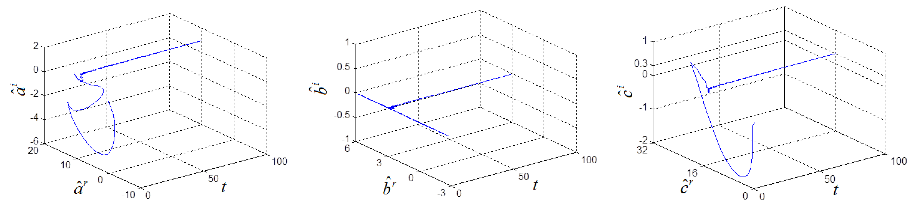
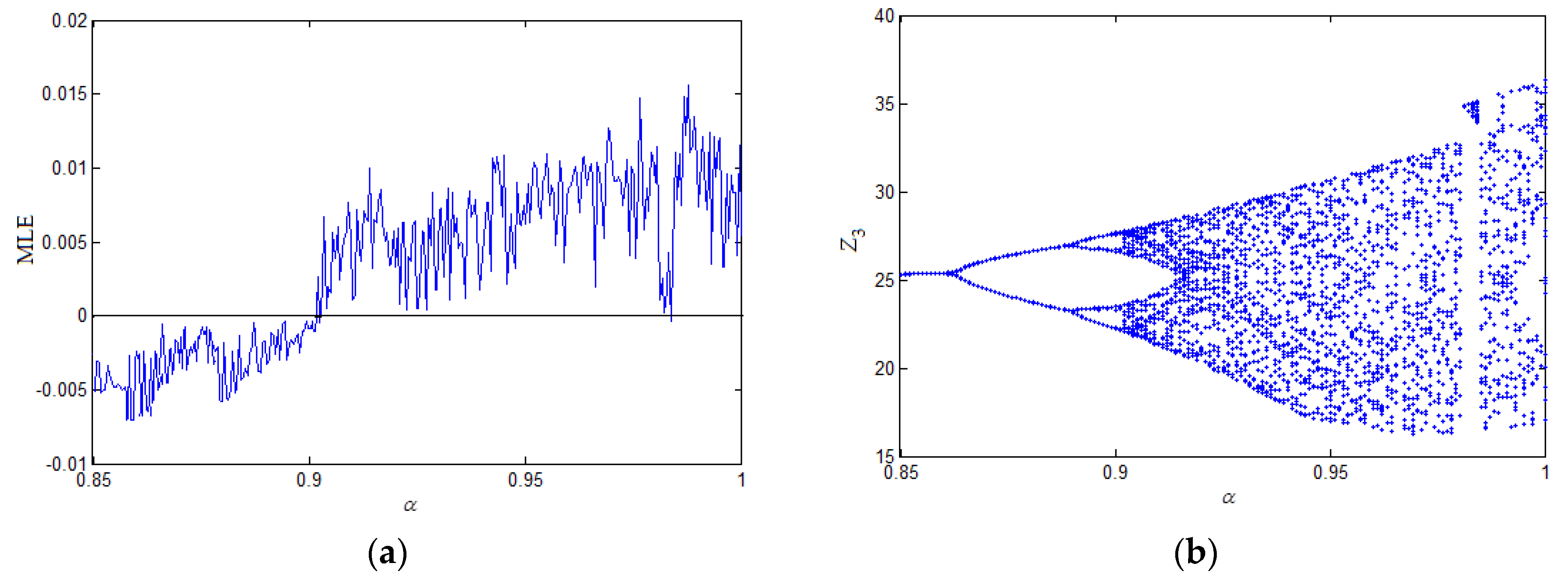
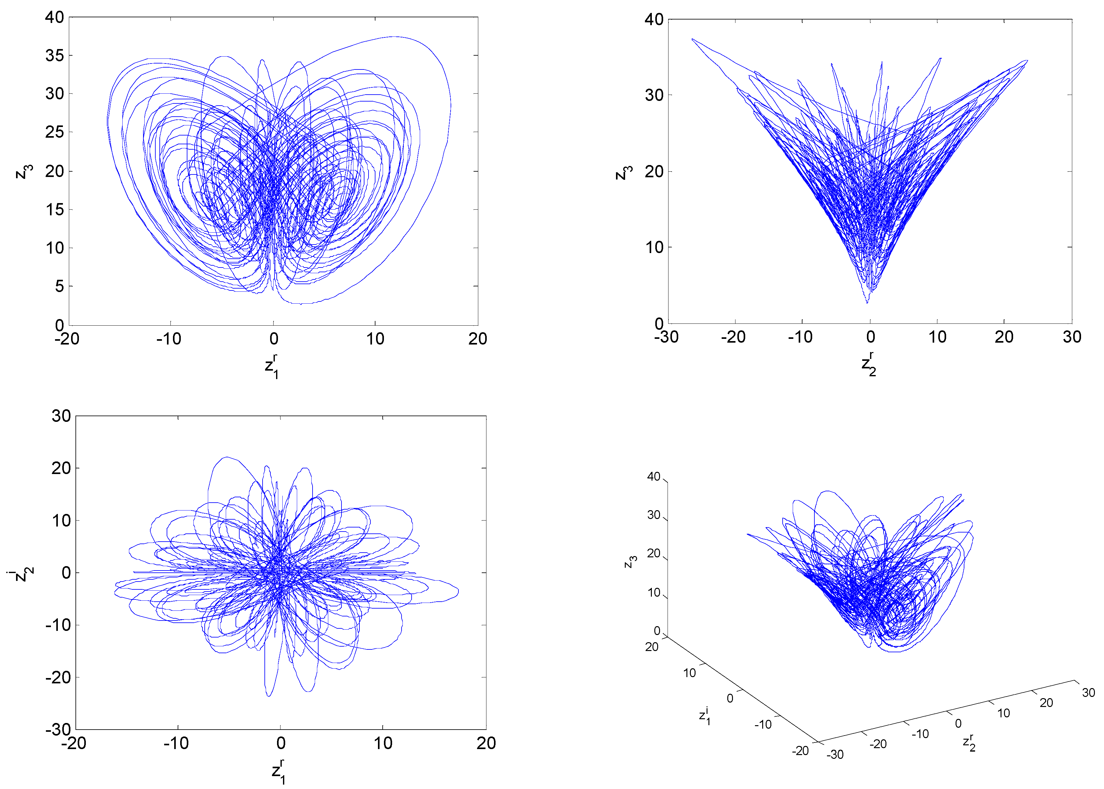
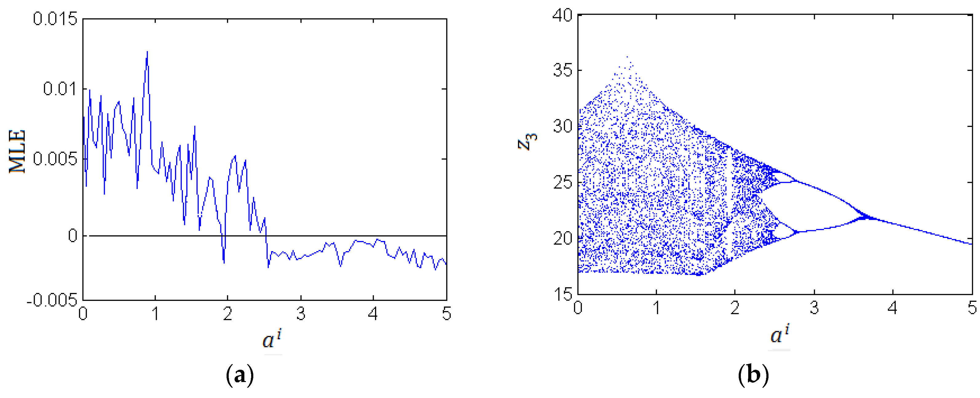
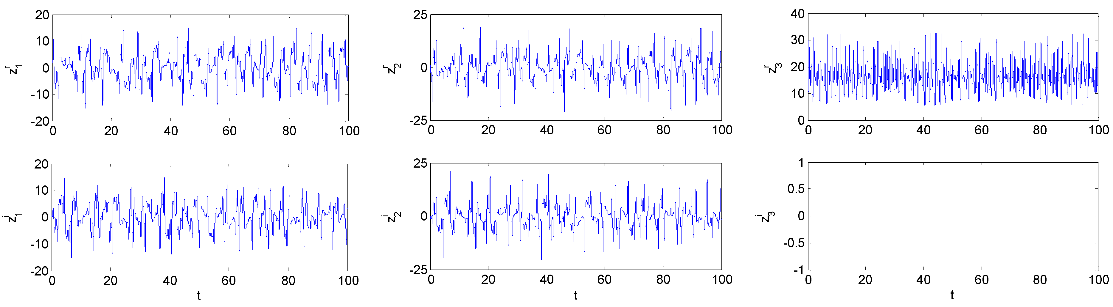
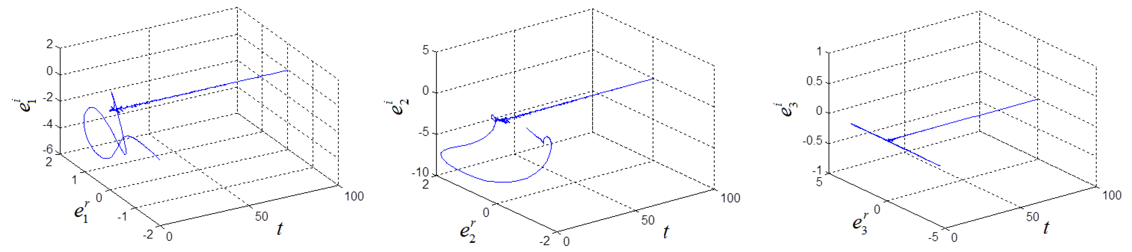
4. Numerical Simulations

In this section, in order to show the effectiveness of the proposed scheme in preceding section, numerical example on fractional-order complex chaotic system will be provided. When numerically solving such systems, we first adopt the predictor–corrector method [40] by MATLAB. Lyapunov exponents of the systems are calculated by adopting the Wolf et al. algorithm [41] with some changes.

Consider the Lorenz-like fractional-order complex chaotic system with commensurate order:

$$\left(\begin{array}{c}{}_0{}^{C}D_t^{\alpha }{z}_1\\ {}_0{}^{C}D_t^{\alpha }{z}_2\\ {}_0{}^{C}D_t^{\alpha }{z}_3\end{array}\right)=\left(\begin{array}{c}a(z_2+z_1)\\ -c{z}_2-z_1{z}_3\\ {\overline{z}}_1{z}_1-b{z}_3\end{array}\right)=\left(\begin{array}{ccc}{z}_2+z_1& 0& 0\\ 0& -z_2& 0\\ 0& 0& -z_3\end{array}\right)\left(\begin{array}{c}a\\ c\\ b\end{array}\right)+\left(\begin{array}{c}0\\ -z_1{z}_3\\ {\overline{z}}_1{z}_1\end{array}\right)$$

(19)

where $z_1,\hspace{0.17em}{z}_2,\hspace{0.17em}{z}_3$ are the complex state variables and a, b, c are system parameters; let $a=10+i,\hspace{0.17em}$$b=3,\hspace{0.17em}c=16+0.3i$. The maximum Lyapunov exponent (MLE) spectrum is depicted in Figure 1a, and the bifurcation diagram is presented in Figure 1b. Figure 1a,b shows that system (19) is chaotic with fractional order $\alpha \in [0.91,0.98]\cup [0.985,1]$ and parameters $a=10+i,\hspace{0.17em}b=3,\hspace{0.17em}c=16+0.3i$. When the fractional-order $\alpha =0.95$, the attractor trajectories are illustrated in Figure 2.

Recently, ref. [42] described how to perform a successful simulation and optimization, and how to synthesize the mathematical models using CMOS technology. The application of metaheuristics to optimize MLE by varying the parameters of the oscillators was discussed.

Field-programmable gate array (FPGA)-based implementation of chaotic oscillators has demonstrated its usefulness in the development of engineering applications in a wide variety of fields, such as: random number generators, robotics and chaotic secure communication systems, signal processing. Very recently, Pano-Azucena et al. [43] implemented the chaotic system using a field-programmable gate array (FPGA) based on trigonometric polynomials. Reference [44] detailed the FPGA-based implementation of all the fractional order chaotic oscillators applying Grünwald-Letnikov(G-L) method. Their work proved experimentally that applying G-L method with 256 elements of memory; it can observe different families of Fractional-order chaotic attractors having working frequencies between 77.59 MHz and 84.9 MHz. This is very beneficial to the development of fractional-order chaos in engineering applications. For the FPGA-based implementation of FOCCS, the FOCCS was first separated into two real-variable systems according to their real and imaginary parts, and then these real-variable systems can be implemented using FPGA by the method proposed by. In order to find much better behavior and characteristics of the FOCCS in the complex domain, we used the G-L method to numerically solve the system (19) again. The MLE spectrum with varying parameter aⁱ (the imaginary of a) is depicted in Figure 3a, the bifurcation diagram is presented in Figure 3b, the state trajectories are illustrated in Figure 4.

Taking the system (19) as master system, and assuming the parameters a, b and c are unknown, the response system is given as follows:

$$\left(\begin{array}{c}{}_0{}^{C}D_t^{\alpha }{w}_1\\ {}_0{}^{C}D_t^{\alpha }{w}_2\\ {}_0{}^{C}D_t^{\alpha }{w}_3\end{array}\right)=\left(\begin{array}{ccc}{w}_2+w_1& 0& 0\\ 0& -w_2& 0\\ 0& 0& -w_3\end{array}\right)\left(\begin{array}{c}\widehat{a}\\ \widehat{c}\\ \widehat{b}\end{array}\right)+\left(\begin{array}{c}0\\ -w_1{w}_3\\ {\overline{w}}_1{w}_1\end{array}\right)+\left(\begin{array}{c}{u}_1\\ u_2\\ u_3\end{array}\right)$$

(20)

where $\widehat{a},\hspace{0.17em}\widehat{b},\hspace{0.17em}\widehat{c}$ are parameter estimations. $u_1,\hspace{0.17em}{u}_2,\hspace{0.17em}{u}_3$ are the controller.

According to Theorem 1, the controllers and the update rules are selected as:

$$\begin{gathered} u_1=-k{e}_1,\hspace{0.17em}{u}_2=-k{e}_2,\hspace{0.17em}{u}_3=-k{e}_3 \\ {}_0{}^{C}D_t^{\alpha }k=\sigma e^{H}e=\sigma ({\overline{e}}_1{e}_1+{\overline{e}}_2{e}_2+{\overline{e}}_3{e}_3),\hspace{0.17em}(\sigma >0) \end{gathered}$$

(21)

$$\left(\begin{array}{c}{}_0{}^{C}D_t^{\alpha }\widehat{a}\\ {}_0{}^{C}D_t^{\alpha }\widehat{c}\\ {}_0{}^{C}D_t^{\alpha }\widehat{b}\end{array}\right)={\left(\begin{array}{ccc}{w}_1+w_2& 0& 0\\ 0& -w_2& 0\\ 0& 0& -w_3\end{array}\right)}^H\left(\begin{array}{c}{e}_1\\ e_2\\ e_3\end{array}\right)=\left(\begin{array}{c}-(w_1+w_2)e_1\\ {\overline{w}}_2{e}_2\\ {\overline{w}}_3{e}_3\end{array}\right)$$

(22)

In the simulation, let $\alpha =0.95$, (a, b, c) = (30 + i, 3, 26 + 0.6i), the initial conditions $z(0)=$ ${(1+i,\hspace{0.17em}-2-i,\hspace{0.17em}6)}^T,\hspace{0.17em}w(0)={(-1+i,\hspace{0.17em}-3+i,\hspace{0.17em}10)}^T,$ $(\widehat{a}(0),\hspace{0.17em}\widehat{b}(0),\hspace{0.17em}\widehat{c}(0))=(20,2,20)$, $k(0)=0$ and $\sigma =6$. Two systems can achieve synchronization and the parameters are identified, as shown in Figure 5 and Figure 6.

5. Conclusions

We studied the adaptive synchronization of FOCCS with unknown complex parameters, and proposed a method for analyzing FOCCS without separating system into real and imaginary parts. By this method, the constructed response system can be asymptotically synchronized to an uncertain drive system with a desired complex scaling diagonal matrix. The proposed synchronization scheme retains the complex nature of fractional-order complex chaotic system. It not only provides a new method of analyzing FOCCS, but also significantly decreases the complexity of computation and analysis. We hope that the work performed will be helpful to further research of nonlinear fractional order complex-variable systems.

References

1. Gorenlo, R.; Mainardi, F. Fractional Calculus; Springer: Berlin, Germany, 1997. [Google Scholar]
2. Caponetto, R. Fractional Order Systems: Modeling and Control Applications; World Scientiic: Singapore, 2010. [Google Scholar]
3. Magin, R.L. Fractional Calculus in Bioengineering; Begell House Redding: New York, NY, USA, 2006. [Google Scholar]
4. Radwan, A.G.; Shamim, A.; Salama, K.N. Theory of fractional order elements based impedance matching networks. IEEE Microwave Wirel. Comp. Lett. 2011, 21, 120–122. [Google Scholar] [CrossRef]
5. Radwan, A.G.; Abd-El-Haiz, S.K.; Abdelhaleem, S.H. Image encryption in the fractional-order domain. In Proceedings of the 1st International Conference on Engineering and Technology, Cairo, Egypt, 10–11 October 2012. [Google Scholar]
6. Kiani-B, A.; Fallah, K.; Pariz, N.; Leung, H. A chaotic secure communication scheme using fractional chaotic systems based on an extended fractional Kalman filter. Commun. Nonlinear Sci. Numer. Simul. 2009, 14, 863–879. [Google Scholar] [CrossRef]
7. Li, G.J.; Liu, H. Stability analysis and synchronization for a class of fractional-order neural networks. Entropy 2016, 18, 55. [Google Scholar] [CrossRef]
8. Yin, C.; Cheng, Y.; Zhong, S.M.; Bai, Z. Fractional-order switching type control law design for adaptive sliding mode technique of 3D fractional-order nonlinear systems. Complexity 2016, 21, 363–373. [Google Scholar] [CrossRef]
9. Liu, H.; Li, S.G.; Wang, H.X.; Huo, Y.H.; Luo, J.H. Adaptive synchronization for a class of uncertain fractional-order neural networks. Entropy 2015, 17, 7185–7200. [Google Scholar] [CrossRef]
10. Lu, J.G. Chaotic dynamics of the fractional-order Lü system and its synchronization. Phys. Lett. A 2006, 354, 305–311. [Google Scholar] [CrossRef]
11. Li, C.G.; Chen, G.R. Chaos in the fractional-order Chen system and it’s control. Chaos Solitons Fractals 2004, 22, 549–554. [Google Scholar] [CrossRef]
12. Agrawal, S.K.; Srivastava, M.; Das, S. Synchronization of fractional order chaotic systems using active control method. Chaos Solitons Fractals 2012, 45, 737–752. [Google Scholar] [CrossRef]
13. Chen, L.P.; Chai, Y.; Wu, R.C. Lag projective synchronization in fractional-order chaotic (hyperchaotic) systems. Phys. Lett. A 2011, 375, 2099–2110. [Google Scholar] [CrossRef]
14. Zhang, Y.; Sun, J. Chaotic synchronization and anti-synchronization based on suitable separation. Phys. Lett. A 2004, 330, 442–447. [Google Scholar] [CrossRef]
15. Zhang, R.X.; Yang, S.P. Robust synchronization of two different fractional-order chaotic systems with unknown parameters using adaptive sliding mode approach. Nonlinear Dyn. 2013, 71, 269–278. [Google Scholar] [CrossRef]
16. Zhang, R.X.; Yang, S.P. Adaptive synchronization of fractional-order chaotic systems via a single driving variable. Nonlinear Dyn. 2011, 66, 831–837. [Google Scholar] [CrossRef]
17. Zhang, R.X.; Yang, S.P. Robust chaos synchronization of fractional-order chaotic systems with unknown parameters and uncertain perturbations. Nonlinear Dyn. 2012, 69, 983–992. [Google Scholar] [CrossRef]
18. Wang, S.; Wang, X.; Han, B. Complex generalized synchronization and parameter identification of nonidentical nonlinear complex systems. PLoS ONE 2016, 11, e0152099. [Google Scholar] [CrossRef] [PubMed]
19. Jiang, C.; Zhang, F.; Li, T. Synchronization and anti-synchronization of N-coupled fractional-order complex chaotic systems with ring connection. Math. Meth. Appl. Sci. 2018, 41, 2625–2638. [Google Scholar] [CrossRef]
20. Zhang, F.F.; Liu, S. Self-time-delay synchronization of time-delay coupled complex chaotic system and its applications to communication. Int. J. Mod. Phys. C 2014, 25, 559–583. [Google Scholar] [CrossRef]
21. Luo, C.; Wang, X.Y. Chaos in the fractional-order complex Lorenz system and its synchronization. Nonlinear Dyn. 2013, 71, 241–257. [Google Scholar] [CrossRef]
22. Luo, C.; Wang, X. Chaos generated from the fractional-order complex Chen system and its application to digital secure communication. Int. J. Mod. Phys. C 2013, 24, 72–77. [Google Scholar] [CrossRef]
23. Liu, X.J.; Hong, L.; Yang, L.X. Fractional-order complex T system: Bifurcations, chaos control, and synchronization. Nonlinear Dyn. 2014, 75, 589–602. [Google Scholar] [CrossRef]
24. Zhang, W.W.; Cao, J.D.; Chen, D.Y.; Alsaadi, F.E. Synchronization in fractional-order complex-valued delayed neural networks. Entropy 2018, 20, 54. [Google Scholar] [CrossRef]
25. Li, L.; Wang, Z.; Lu, J.W.; Li, Y.X. Adaptive synchronization of fractional-order complex-valued neural networks with discrete and distributed delays. Entropy 2018, 20, 124. [Google Scholar] [CrossRef]
26. Sun, J.; Deng, W.; Cui, G.Z.; Wang, Y.F. Real combination synchronization of three fractional-order complex-variable chaotic systems. Optik 2016, 127, 11460–11468. [Google Scholar] [CrossRef]
27. Yadav, V.K.; Srikanth, N.; Das, S. Dual function projective synchronization of fractional order complex chaotic systems. Optik 2016, 127, 10527–10538. [Google Scholar] [CrossRef]
28. Nian, F.Z.; Liu, X.M.; Zhang, Y. Sliding mode synchronization of fractional-order complex chaotic system with parametric and external disturbances. Chaos Solitons Fractals 2018, 116, 22–28. [Google Scholar] [CrossRef]
29. Jiang, C.M.; Liu, S.T.; Zhang, F.F. Complex modified projective synchronization for fractional-order chaotic complex systems. Int. J. Auto Comput. 2017, 15, 603–615. [Google Scholar] [CrossRef]
30. Podlubny, I. Fractional Differential Equations; Academic Press: New York, NY, USA, 1999. [Google Scholar]
31. Aguila-Camacho, N.; Duarte-Mermoud, M.A.; Gallegos, J.A. Lyapunov functions for fractional order systems. Commun. Nonlinear Sci. Numer. Simulat. 2014, 19, 2951–2957. [Google Scholar] [CrossRef]
32. Quan, X.; Zhuang, S.; Liu, S.; Xiao, J. Decentralized adaptive coupling synchronization of fractional-order complex-variable dynamical networks. Neurocomputing 2016, 186, 119–126. [Google Scholar]
33. Zhang, R.X.; Liu, Y. A new Barbalat’s Lemma and Lyapunov stability theorem for fractional order systems. In Proceedings of the 29th Chinese Control and Decision Conference, Chongqing, China, 28–30 May 2017; pp. 3676–3681. [Google Scholar]
34. Wang, F.; Yang, Y.Q. Fractional order Barbalat’s Lemma and its applications in the stability of fractional order nonlinear systems. Math. Model. Anal. 2017, 22, 503–513. [Google Scholar] [CrossRef]
35. Wang, C. Adaptive fuzzy control for uncertain fractional-order financial chaotic systems subjected to input saturation. PLoS ONE 2016, 11, e0164791. [Google Scholar] [CrossRef]
36. Xu, Q.; Xu, X.H.; Zhuang, S.X.; Xiao, J.X.; Song, C.H. New complex projective synchronization strategies for drive-response networks with fractional complex-variable dynamics. Appl. Math. Comput. 2018, 338, 552–566. [Google Scholar] [CrossRef]
37. Tao, F.; Sun, J.T. Stability of complex-valued impulsive system with delay. Appl. Math. Comput. 2014, 240, 102–108. [Google Scholar]
38. Wu, Z.Y.; Chen, G.R.; Fu, X.C. Synchronization of a network coupled with complex-variable chaotic systems. Chaos 2012, 22, 023127. [Google Scholar] [CrossRef]
39. Gu, Y.; Yu, Y.; Wang, H. Synchronization-based parameter estimation of fractional-order neural networks. Physica A Stat. Mech. Appl. 2017, 483, 351–361. [Google Scholar] [CrossRef]
40. Diethelm, K.; Neville, J.F.; Freed, A.D. A predictor-corrector approach for the numerical solution of fractional differential equations. Nonlinear Dyn. 2002, 29, 1–4. [Google Scholar] [CrossRef]
41. Wolf, A.; Swift, J.B.; Swinney, H.L.; Vastano, J.A. Determining Lyapunov exponents from a time series. Physica D 1985, 16, 285–317. [Google Scholar] [CrossRef]
42. Carbajal-Gomez, V.H.; Tlelo-Cuautle, E.; Muñoz-Pacheco, J.M.; de la Fraga, L.G.; Sanchez-Lopez, C.; Fernandez-Fernandez, F.V. Optimization and CMOS design of chaotic oscillators robust to PVT variations: INVITED (In Press). Integration 2018. [Google Scholar] [CrossRef]
43. Pano-Azucena, A.D.; Tlelo-Cuautle, E.; Rodriguez-Gomez, G. de la Fraga, L.G. FPGA-based implementation of chaotic oscillators by applying the numerical method based on trigonometric polynomials. AIP Adv. 2018, 8, 075217. [Google Scholar] [CrossRef]
44. Pano-Azucena, A.D.; Ovilla-Martinez, B.; Tlelo-Cuautle, E.; Muñoz-Pacheco, J.M.; de la Fraga, L.G. FPGA-based implementation of different families of fractional-order chaotic oscillators applying Grounwald-Letnikov method. Commun. Nonlinear Sci. Numer. Simulat. 2019, 72, 516–527. [Google Scholar] [CrossRef]
45. Bao, H.; Park, J.H.; Cao, J. Adaptive synchronization of fractional-order memristor-based neural networks with time delay. Nonlinear Dyn. 2015, 82, 1343–1354. [Google Scholar] [CrossRef]
Figure 1. Dynamic behaviors of the fractional-order complex Lorenz-like System with commensurate order α ( a = 10 + i , b = 3 , c = 16 + 0.3 i ). (a) maximal Lyapunov exponent; (b) bifurcation diagram.
Entropy 21 00207 g001
Figure 2. Chaotic attractors of fractional-order complex Lorenz-like system with a = 10 + i , b = 3 , c = 16 + 0.3 i and commensurate order α = 0.95 .
Entropy 21 00207 g002
Figure 3. Dynamic behaviors of the fractional-order complex Lorenz-like System with commensurate order 0.95 ( a r = 10 , b = 3 , c = 16 + 0.3 i ). (a) maximal Lyapunov exponent; (b) bifurcation diagram.
Entropy 21 00207 g003
Figure 4. The state trajectories of fractional-order complex Lorenz-like system with a = 10 + i , b = 3 , c = 16 + 0.3 i and commensurate order α = 0.95 .
Entropy 21 00207 g004
Figure 5. Synchronization errors e1, e2, e3 of fractional-order complex Lorenz-like chaotic system.
Entropy 21 00207 g005
Figure 6. Estimated complex parameters of fractional-order complex Lorenz-like chaotic system.
Entropy 21 00207 g006