Empirical Mode Decomposition as a Novel Approach to Study Heart Rate Variability in Congestive Heart Failure Assessment


Abstract
:1. Introduction
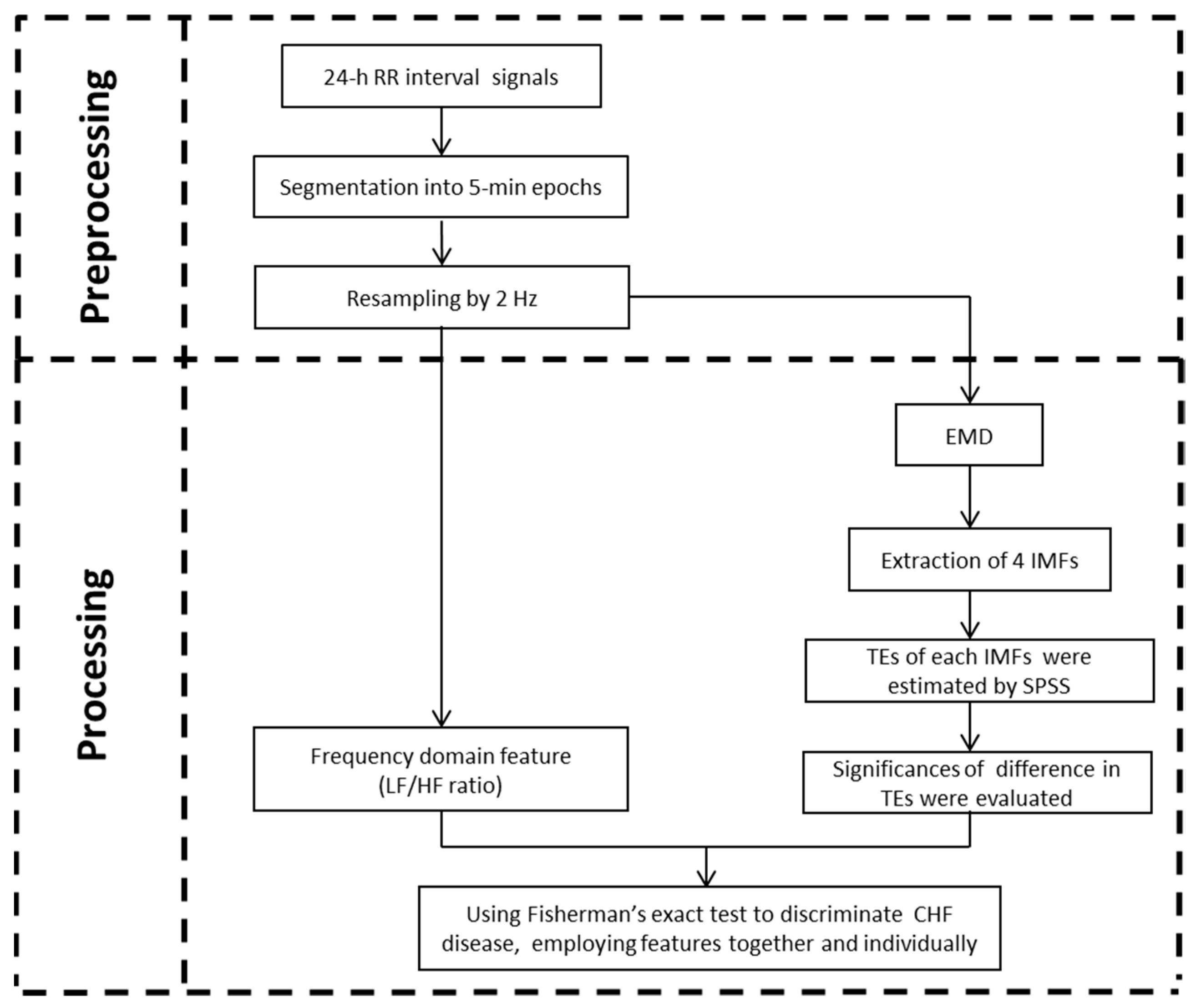
2. Methods
2.1. Data
2.2. HRV Analysis
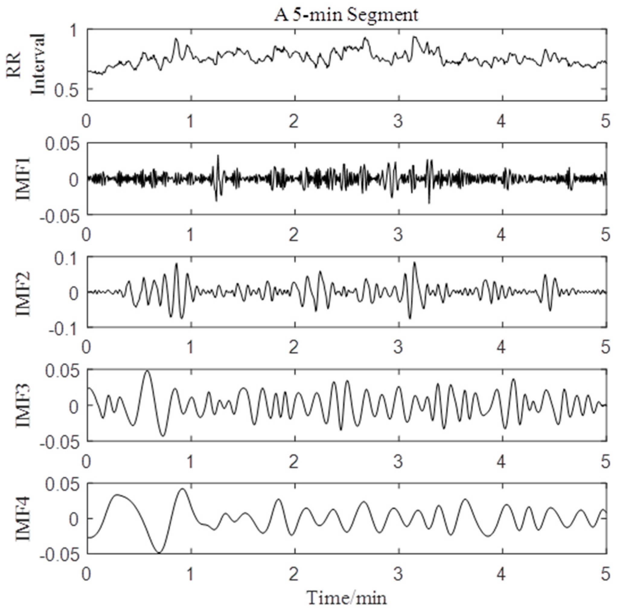
2.2.1. Empirical Model Decomposition
- 1.
- is represented as with subscript j represents the number of IMF and subscript k represents the time of sifting process to get ;
- 2.
- Identify all the local maxima and minima and use cubic fitting to obtain upper envelope and lower envelope of . Then the mean values are calculated by;
- 3.
- The detail is computed byIf meets the two requirements mentioned above,If not, repeat steps 2–3.
- 4.
- To find more IMF components of input data, is calculated byIf is monotone, the residual signalThe origin signal can be shown asIf not, repeat steps 2–4.
2.2.2. Indices Calculation
2.2.3. Simulated Data of EMD
2.3. Statistical Analysis
3. Results
3.1. Simulated Analysis by EMD
3.2. HRV Analysis by EMD
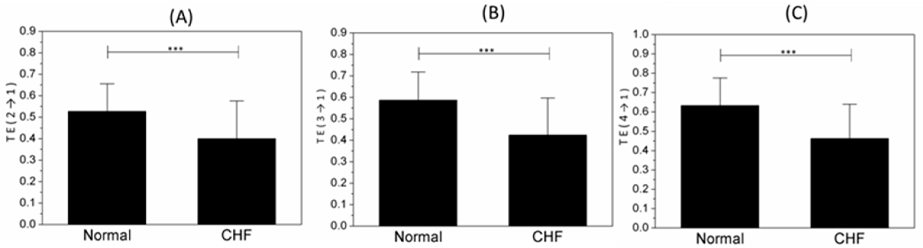
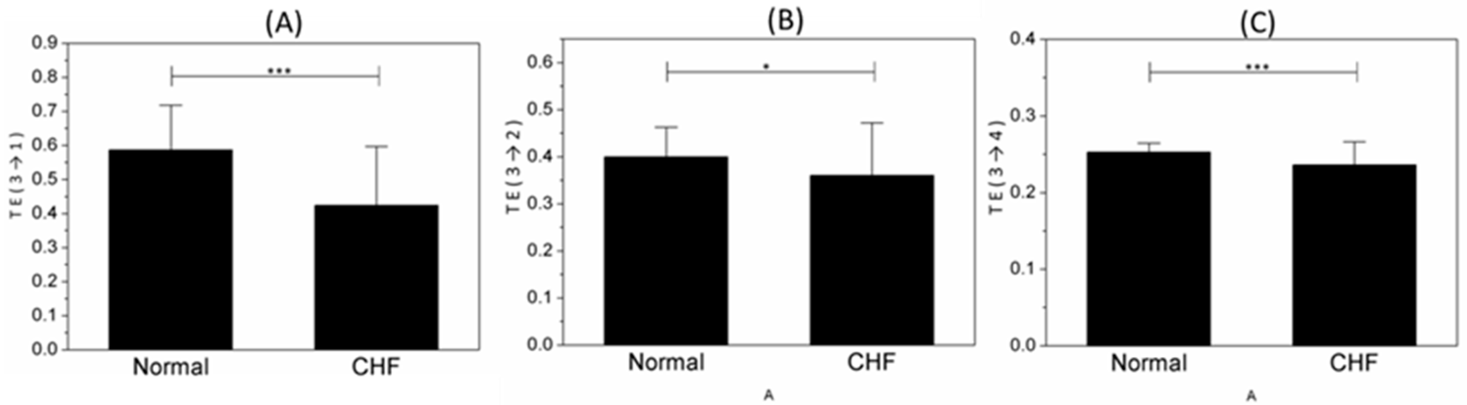
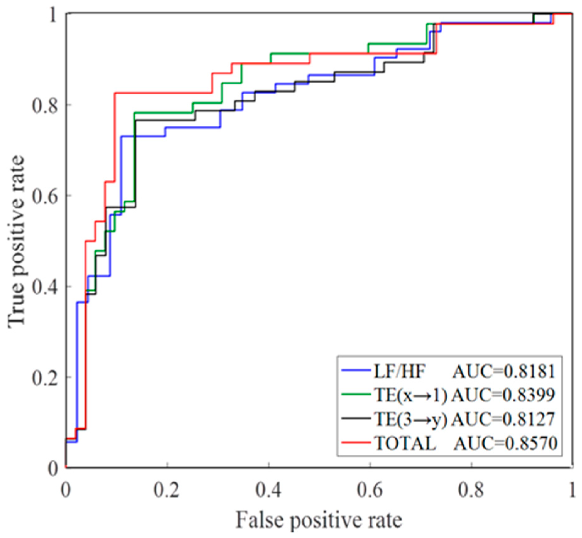
3.3. Disease Analysis by TE
4. Discussion
4.1. Motivation of EMD
4.2. Analysis of IMFs
4.3. Physiological Significance
4.4. Limitation
5. Conclusions
Author Contributions
Funding
Acknowledgments
Conflicts of Interest
References
- Keith, J.D. Congestive heart failure. Pediatrics 1956, 18, 491. [Google Scholar] [PubMed]
- Kumar, M.; Pachori, R.B.; Acharya, U.R. Use of Accumulated Entropies for Automated Detection of Congestive Heart Failure in Flexible Analytic Wavelet Transform Framework Based on Short-Term HRV Signals. Entropy 2017, 19, 92. [Google Scholar] [CrossRef]
- Athena, P.; Sharon, R. Congestive heart failure. Am. J. Respir. Crit. Care Med. 2002, 165, 4. [Google Scholar]
- Chen, W.; Zheng, L.; Li, K.; Wang, Q.; Liu, G.; Jiang, Q. A Novel and Effective Method for Congestive Heart Failure Detection and Quantification Using Dynamic Heart Rate Variability Measurement. PLoS ONE 2016, 11, e0165304. [Google Scholar] [CrossRef]
- Costa, M.D.; Davis, R.B.; Goldberger, A.L. Heart Rate Fragmentation: A New Approach to the Analysis of Cardiac Interbeat Interval Dynamics. Front. Physiol. 2017, 8, 255. [Google Scholar] [CrossRef]
- Pecchia, L.; Melillo, P.; Sansone, M.; Bracale, M. Discrimination Power of Short-Term Heart Rate Variability Measures for CHF Assessment. IEEE Trans. Inf. Technol. Biomed. 2011, 15, 40–46. [Google Scholar] [CrossRef]
- Khoo, M.C.; Kim, T.; Berry, R.B. Spectral indices of cardiac autonomic function in obstructive sleep apnea. Sleep 1999, 22, 443–451. [Google Scholar] [CrossRef]
- Wang, H.; Kuo, T.B.J.; Chan, S.H.H.; Tsai, T.H.; Lee, Y.H.; Lui, P.W. Spectral Analysis of Arterial Pressure Variability During Introduction of Propofol Anesthesia. Anesth. Analg. 1996, 82, 914–919. [Google Scholar]
- Binkley, P.F.; Nunziata, E.; Haas, G.J.; Nelson, S.D.; Cody, R.J. Parasympathetic withdrawal is an integral component of autonomic imbalance in congestive heart failure: Demonstration in human subjects and verification in a paced canine model of ventricular failure. J. Am. Coll. Cardiol. 1991, 18, 464–472. [Google Scholar] [CrossRef]
- Bailón, R.; Mateo, J.; Olmos, S.; Serrano, P.; Garcia, J.; Del Rio, A.; Ferreira, I.J.; Laguna, P.; Rio, A. Coronary artery disease diagnosis based on exercise electrocardiogram indexes from repolarisation, depolarisation and heart rate variability. Med. Biol. Eng. 2003, 41, 561–571. [Google Scholar] [CrossRef]
- Hadase, M.; Azuma, A.; Zen, K.; Asada, S.; Kawasaki, T.; Kamitani, T.; Kawasaki, S.; Sugihara, H.; Matsubara, H. Very low frequency power of heart rate variability is a powerful predictor of clinical prognosis in patients with congestive heart failure. Circ. J. 2004, 68, 343–347. [Google Scholar] [CrossRef] [PubMed]
- Saul, J.P.; Arai, Y.; Berger, R.D.; Lilly, L.S.; Colucci, W.S.; Cohen, R.J. Assessment of autonomic regulation in chronic congestive heart failure by heart rate spectral analysis. Am. J. Cardiol. 1988, 61, 1292–1299. [Google Scholar] [CrossRef]
- Kaur, B.T. Effect of Different Phases of Menstrual Cycle on Heart Rate Variability (HRV). J. Clin. Diagn. Res. 2015, 9. [Google Scholar] [CrossRef]
- Burr, R.L. Interpretation of normalized spectral heart rate variability indices in sleep research: A critical review. Sleep 2007, 30, 913–919. [Google Scholar] [CrossRef] [PubMed]
- Berntson, G.G.; Bigger, J.T., Jr.; Eckberg, D.L.; Grossman, P.; Kaufmann, P.G.; Malik, M.; Nagaraja, H.N.; Porges, S.W.; Saul, J.P.; Stone, P.H.; et al. Heart rate variability: Origins, methods, and interpretive caveats. Psychophysiology 1997, 34, 623–648. [Google Scholar] [CrossRef] [PubMed]
- Stein, P.K.; Domitrovich, P.P.; Hui, N.; Rautaharju, P.; Gottdiener, J. Sometimes higher heart rate variability is not better heart rate variability: A result of graphical and nonlinear analyses. J. Cardiovasc. Electrophysiol. 2005, 16, 954–959. [Google Scholar] [CrossRef]
- Luo, D.; Pan, W.; Li, Y.; Feng, K.; Liu, G. The Interaction Analysis between the Sympathetic and Parasympathetic Systems in CHF by Using Transfer Entropy Method. Entropy 2018, 20, 795. [Google Scholar] [CrossRef]
- Zheng, L.; Pan, W.; Li, Y.; Luo, D.; Wang, Q.; Liu, G. Use of Mutual Information and Transfer Entropy to Assess Interaction between Parasympathetic and Sympathetic Activities of Nervous System from HRV. Entropy 2017, 19, 489. [Google Scholar] [CrossRef]
- Fisher, A.C.; Eleuteri, A.; Groves, D.; Dewhurst, C.J. The Ornstein–Uhlenbeck third-order Gaussian process (OUGP) applied directly to the un-resampled heart rate variability (HRV) tachogram for detrending and low-pass filtering. Med. Biol. Eng. 2012, 50, 737–742. [Google Scholar] [CrossRef]
- Karthikeyan, P.; Murugappan, M.; Yaacob, S. Detection of human stress using short-term ecg and hrv signals. J. Mech. Med. Biol. 2013, 13, 1350038. [Google Scholar] [CrossRef]
- Myers, G.; Workman, M.; Birkett, C.; Ferguson, D.; Kienzle, M. Problems in measuring heart rate variability of patients with congestive heart failure. J. Electrocardiol. 1992, 25, 214–219. [Google Scholar] [CrossRef]
- Huang, N.E.; Shen, Z.; Long, S.R.; Wu, M.C.; Shih, H.H.; Zheng, Q.; Yen, N.C.; Tung, C.C.; Liu, H.H. The empirical mode decomposition and the hilbert spectrum for nonlinear and non-stationary time series analysis. Proc. R. Soc. A Math. Phys. Eng. Sci. 1971, 454, 903–995. [Google Scholar] [CrossRef]
- Thameur, K.; Raynald, G.; Mohamed, E.B.; Marc, T. Comparison between the efficiency of L.M.D and E.M.D algorithms for early detection of gear defects. Mech. Ind. 2013, 14, 121–127. [Google Scholar] [CrossRef]
- Abu Anas, E.M.; Lee, S.Y.; Hasan, M.K. Exploiting correlation of ECG with certain EMD functions for discrimination of ventricular fibrillation. Comput. Biol. Med. 2011, 41, 110–114. [Google Scholar] [CrossRef] [PubMed]
- Pan, W.; He, A.; Feng, K.; Li, Y.; Wu, D.; Liu, G. Multi-Frequency Components Entropy as Novel Heart Rate Variability Indices in Congestive Heart Failure Assessment. IEEE Access 2019, 7, 37708–37717. [Google Scholar] [CrossRef]
- Luca, F.; Daniele, M.; Alessandro, M.; Giandomenico, N. Lag-specific transfer entropy as a tool to assess cardiovascular and cardiorespiratory information transfer. IEEE Trans. Biomed. Eng. 2014, 61, 2556–2568. [Google Scholar]
- Zheng, L.; Li, Y.; Chen, W.; Wang, Q.; Jiang, Q.; Liu, G. Detection of Respiration Movement Asymmetry Between the Left and Right Lungs Using Mutual Information and Transfer Entropy. IEEE Access 2017, 6, 605–613. [Google Scholar] [CrossRef]
- Krum, H.; Bigger, T.; Goldsmith, R.L.; Packer, M. Effect of long-term digoxin therapy on autonomic function in patients with chronic heart failure. J. Am. Coll. Cardiol. 1995, 25, 289–294. [Google Scholar] [CrossRef]
- Task Force of the European Society of Cardiology the North American Society of Pacing Electrophysiology. Heart rate variability: Standards of measurement, physiological interpretation, and clinical use. Circulation 1996, 93, 354–381. [Google Scholar]
- Takase, B.; Kurita, A.; Noritake, M.; Uehata, A.; Maruyama, T.; Nagayoshi, H.; Nishioka, T.; Mizuno, K.; Nakamura, H. Heart rate variability in patients with diabetes mellitus, ischemic heart disease, and congestive heart failure. J. Electrocardiol. 1992, 25, 79–88. [Google Scholar] [CrossRef]
- Boudraa, A.O.; Cexus, J.C. EMD-Based Signal Filtering. IEEE Trans. Instrum. Meas. 2007, 56, 2196–2202. [Google Scholar] [CrossRef]
- Wang, Y.; He, Z.; Zi, Y. A Comparative Study on the Local Mean Decomposition and Empirical Mode Decomposition and Their Applications to Rotating Machinery Health Diagnosis. J. Vib. Acoust. 2010, 132. [Google Scholar] [CrossRef]
- Li, Y.; Pan, W.; Li, K.; Jiang, Q.; Liu, G.Z. Sliding Trend Fuzzy Approximate Entropy as a Novel Descriptor of Heart Rate Variability in Obstructive Sleep Apnea. IEEE J. Biomed. Health Inform. 2018, 23, 175–183. [Google Scholar] [CrossRef] [PubMed]
- Marzbanrad, F.; Kimura, Y.; Endo, M.; Palaniswami, M.; Khandoker, A.H. Transfer entropy analysis of maternal and fetal heart rate coupling. In Proceedings of the 2015 37th Annual International Conference of the IEEE Engineering in Medicine and Biology Society (EMBC), Milan, Italy, 25–29 August 2015; pp. 7865–7868. [Google Scholar]
- Lindner, M.; Vicente, R.; Priesemann, V.; Wibral, M. TRENTOOL: A Matlab open source toolbox to analyse information flow in time series data with transfer entropy. BMC Neurosci. 2011, 12, 119. [Google Scholar] [CrossRef] [PubMed]
- Liu, G.; Lei, W.; Wang, Q.; Zheng, G.; Ying, W.; Jiang, Q. A new approach to detect congestive heart failure using short-term heart rate variability measures. PLoS ONE 2014, 9, e93399. [Google Scholar] [CrossRef]
- Acharya, U.R.; Fujita, H.; Sudarshan, V.K.; Oh, S.L.; Muhammad, A.; Koh, J.E.W.; Tan, J.H.; Chua, C.K.; Chua, K.P.; Tan, R.S. Application of empirical mode decomposition (EMD) for automated identification of congestive heart failure using heart rate signals. Neural Comput. Appl. 2017, 28, 3073–3094. [Google Scholar] [CrossRef]
- Chen, Y.; Ma, J. Random noise attenuation by f-x empirical-mode decomposition predictive filtering. Geophysics 2014, 79, V81–V91. [Google Scholar] [CrossRef]
- Pyetan, E.; Akselrod, S. Do the high-frequency indexes of HRV provide a faithful assessment of cardiac vagal tone? A critical theoretical evaluation. IEEE Trans. Biomed. Eng. 2003, 50, 777–783. [Google Scholar] [CrossRef]
- Alberto, P.; Stefano, G.; Ester, B.; Raffaello, F.; Nicola, M.; Alberto, M. Role of the autonomic nervous system in generating non-linear dynamics in short-term heart period variability. Biomed. Eng. Biomed. Tech. 2006, 51, 174–177. [Google Scholar]
- Shafqat, K.; Pal, S.K.; Kumari, S.; Kyriacou, P.A. Empirical mode decomposition (EMD) analysis of HRV data from locally anesthetized patients. In Proceedings of the 2009 Annual International Conference of the IEEE Engineering in Medicine and Biology Society, Minneapolis, MN, USA, 3–6 September 2009; pp. 2244–2247. [Google Scholar]
- Bajaj, V.; Pachori, R.B. Separation of Rhythms of EEG Signals Based on Hilbert-Huang Transformationwith Application to Seizure Detection. In Proceedings of the Computer Vision—ECCV 2012; Springer Science and Business Media LLC: Berlin/Heidelberg, Germany, 2012; Volume 7425, pp. 493–500. [Google Scholar]
- Duprez, D.; De Buyzere, M.; Rietschel, E.; Rimbout, S.; Kaufman, J.M.; Van Hoecke, M.J.; Clement, D.L. Renin-angiotensin-aldosterone system, RR-interval and blood pressure variability during postural changes after myocardial infraction. Eur. Heart J. 1995, 16, 1050–1056. [Google Scholar] [CrossRef]
- Francis, D.P.; Davies, L.C.; Willson, K.; Ponikowski, P.; Coats, A.J.S.; Piepoli, M. Very-low-frequency oscillations in heart rate and blood pressure in periodic breathing: Role of the cardiovascular limb of the hypoxic chemoreflex. Clin. Sci. 2000, 99, 125–132. [Google Scholar] [CrossRef] [PubMed]
- Arutyunov, G.; Rylova, N.; Rylova, A.; Serov, R.; Pokrovsky, Y. 342 Correction of morpho-functional disorders in skeletal muscles of patients with CHF. Eur. J. Heart Fail. Suppl. 2015, 2, 65. [Google Scholar] [CrossRef]
- Vincenza, S.; Dan, Z.; Roy, F.; Luciano, B.; Simona, F.; Rodica, P.B.; Martin, S.; Peter, K.; Jannik, H.; Solomon, T. Cardiovascular autonomic neuropathy in diabetes: Clinical impact, assessment, diagnosis, and management. Diabetes Metab. Res. Rev. 2011, 27, 639–653. [Google Scholar]
- Sinha, A.N.; Deepak, D.; Gusain, V.S. Assessment of the effects of pranayama/alternate nostril breathing on the parasympathetic nervous system in young adults. J. Clin. Diagn. Res. 2013, 7, 821–823. [Google Scholar] [CrossRef]
- Rovere, M.T.L.; Pinna, G.D.; Roberto, M.; Andrea, M.; Soccorso, C.; Oreste, F.; Roberto, F.; Mariella, F.; Marco, G.; Cristina, O. Short-term heart rate variability strongly predicts sudden cardiac death in chronic heart failure patients. Circulation 2003, 107, 565–570. [Google Scholar] [CrossRef]
- Goto, T.; Fukushima, H.; Sasaki, G.; Matsuo, N.; Takahashi, T. Evaluation of autonomic nervous system function with spectral analysis of heart rate variability in a case of tetanus. Brain Dev. 2001, 23, 791–795. [Google Scholar] [CrossRef]


| Indices | Normal (Mean ± SD) | CHF (Mean ± SD) | p-Value |
|---|---|---|---|
| TE (2→1) | 0.5275 ± 0.12805 | 0.3995 ± 0.17607 | 0.000 *** |
| TE (1→2) | 0.3523 ± 0.08306 | 0.3313 ± 0.13262 | 0.364 |
| TE (3→1) | 0.5866 ± 0.13141 | 0.4245 ± 0.17261 | 0.000 *** |
| TE (1→3) | 0.2664 ± 0.03964 | 0.2531 ± 0.07634 | 0.299 |
| TE (4→1) | 0.6323 ± 0.14308 | 0.4625 ± 0.17730 | 0.000 *** |
| TE (1→4) | 0.2161 ± 0.02868 | 0.2010 ± 0.04566 | 0.060 |
| TE (3→2) | 0.3999 ± 0.06272 | 0.3600 ± 0.11196 | 0.039 * |
| TE (2→3) | 0.2770 ± 0.03107 | 0.2623 ± 0.06932 | 0.198 |
| TE (4→2) | 0.4283 ± 0.06653 | 0.3972 ± 0.10781 | 0.099 |
| TE (2→4) | 0.2205 ± 0.01821 | 0.2102 ± 0.03837 | 0.109 |
| TE (4→3) | 0.3442 ± 0.02340 | 0.3269 ± 0.05502 | 0.056 |
| TE (3→4) | 0.2526 ± 0.01196 | 0.2359 ± 0.03023 | 0.001 *** |
| Indices | Acc (%) | Sen (%) | Spe (%) |
|---|---|---|---|
| LF/HF | 79.6 | 86.4 | 74.1 |
| TE (2→1) | 69.4 | 70.5 | 68.5 |
| TE (3→1) | 70.4 | 70.5 | 70.4 |
| TE (4→1) | 70.4 | 70.5 | 70.4 |
| TE (3→2) | 63.3 | 63.6 | 63.0 |
| TE (3→4) | 78.6 | 75.0 | 81.5 |
| TE (2→1) and TE (3→1) and TE (4→1) | 81.6 | 81.8 | 81.5 |
| TE (3→1) and TE (3→2) and TE (3→4) | 80.6 | 81.8 | 79.6 |
| LF/HF and TE (2→1) and TE (3→1) and TE (4→1) and TE (3→2) and TE (3→4) | 85.7 | 86.4 | 85.2 |
| Symbol | MIF ± SD (Hz) | Frequency Band |
|---|---|---|
| IMF1 | 0.431 ± 0.152 | VHF |
| IMF2 | 0.199 ± 0.081 | HF |
| IMF3 | 0.076 ± 0.037 | LF |
| IMF4 | 0.027 ± 0.012 | VLF |
© 2019 by the authors. Licensee MDPI, Basel, Switzerland. This article is an open access article distributed under the terms and conditions of the Creative Commons Attribution (CC BY) license (http://creativecommons.org/licenses/by/4.0/).
Share and Cite
Chen, M.; He, A.; Feng, K.; Liu, G.; Wang, Q. Empirical Mode Decomposition as a Novel Approach to Study Heart Rate Variability in Congestive Heart Failure Assessment. Entropy 2019, 21, 1169. https://doi.org/10.3390/e21121169
Chen M, He A, Feng K, Liu G, Wang Q. Empirical Mode Decomposition as a Novel Approach to Study Heart Rate Variability in Congestive Heart Failure Assessment. Entropy. 2019; 21(12):1169. https://doi.org/10.3390/e21121169
Chicago/Turabian StyleChen, Mingjing, Aodi He, Kaicheng Feng, Guanzheng Liu, and Qian Wang. 2019. "Empirical Mode Decomposition as a Novel Approach to Study Heart Rate Variability in Congestive Heart Failure Assessment" Entropy 21, no. 12: 1169. https://doi.org/10.3390/e21121169
APA StyleChen, M., He, A., Feng, K., Liu, G., & Wang, Q. (2019). Empirical Mode Decomposition as a Novel Approach to Study Heart Rate Variability in Congestive Heart Failure Assessment. Entropy, 21(12), 1169. https://doi.org/10.3390/e21121169