Entropy Analysis in Double-Diffusive Convection in Nanofluids through Electro-Osmotically Induced Peristaltic Microchannel

Abstract

A theoretical study is presented to examine entropy generation in double-diffusive convection in an Electro-osmotic flow (EOF) of nanofluids via a peristaltic microchannel. Buoyancy effects due to change in temperature, solute concentration and nanoparticle volume fraction are also considered. This study was performed under lubrication and Debye-Hückel linearization approximation. The governing equations are solved exactly. The effect of dominant hydrodynamic parameters (thermophoresis, Brownian motion, Soret and Dufour), Grashof numbers (thermal, concentration and nanoparticle) and electro-osmotic parameters on double-diffusive convective flow are discussed. Moreover, trapping, pumping, entropy generation number, Bejan number and heat transfer rate were also examined under the influence of pertinent parameters such as the thermophoresis parameter, the Brownian motion parameter, the Soret parameter, the Dufour parameter, the thermal Grashof number, the solutal Grashof number, the nanoparticle Grashof number, the electro-osmotic parameter and Helmholtz–Smoluchowski velocity. The electro-osmotic parameter powerfully affected the velocity profile. The magnitude of total entropy generation increased as the thermophoresis parameter and Brownian motion parameter increased. Soret and the Dufour parameter had a strong tendency to control the temperature profile and Bejan number. The findings of the present analysis can be used in clinical purposes such as cell therapy, drug delivery systems, pharmaco-dynamic pumps and particles filtration.

1. Introduction

In 1809, Resuss [1] illustrated an electrokinetic phenomenon known as electroosmosis or Electro-osmotic flow (EOF). It is defined as the flow of fluid in any conduit (e.g., microchannel, capillary tube) under the effect of the external electric field. EOF has many applications in micro-flow injection analysis, micro-liquid chromatography and micro-energy system. Patankar et al. [2] investigated the behavior of electro-osmotic flow through a microchannel. Yang et al. [3] studied the EOF in microfluidics. Tang et al. [4] scrutinized the EOF for a Power-law model. Later, Miller et al. [5] predicted EOF through a carbon nanotube membrane.

Peristaltic transport of a fluid is a special type of fluid transport that occurs due to the propagation of progressive waves of area contraction/expansion. This is a natural process of transport in living beings. The literature reveals that different studies have explained this phenomenon under various impacts. Some recent readings are cited in [6,7,8,9,10,11].

Nanofluids have been found to exhibit enhanced thermophysical properties (thermal conductivity, thermal diffusivity, the viscosity of convective heat transport coefficient) compared to base fluids. Nanofluids dynamics have shown tremendous potential applications in many fields. The endoscopic impact of nanofluid in peristalsis was analyzed by Akbar et al. [12]. Noreen [13] investigated nanofluids under induced magnetic field and mixed convection. Furthermore, Tripathi et al. [14] studied the peristaltic motion of nanofluid. Reddy et al. [15] recommended the peristaltic flow of nanofluid through complaint walls. Ebaid et al. [16] examined the peristaltic motion of nanofluid with convective conditions.

Shao et al. [17] studied a reference solution for double-diffusion convection. Double-diffusive convection is a fluid dynamics phenomenon that describes a form of convection driven by two different density gradients (temperature and concentration) that have different diffusion rates. If the temperature difference is held constant, thermal diffusion produces a concentration gradient. Considering the wide applications of double-diffusive convection, it was studied in a nanofluidic flow model with peristaltic pumping. Huppert et al. [18] discussed the applications of double-diffusion convection. Similarly, Bég et al. [19] described the peristaltic pumping of nanofluids through double-diffusive convection. Kefayati [20] explained double-diffusion convection for pseudoplastic fluids. The peristaltic motion of MHD flow through double-diffusive convection was studied by Rout et al. [21]. Gaffar et al. [22] observed the double-diffusive convection under the effect of heat absorption. Furthermore, Mohan et al. [23] also described the influence of double-diffusive convection in a lid-driven cavity.

Peristaltic flow and EOF have guaranteed biomedical and engineering applications. Today, the collective effect of peristalsis and electroosmosis is of supreme importance in many applications, such as biomicrofluidic devices and biomimetic pumping. Some mathematical models with various physical applications and various flow regimes have been studied. Bandopadhyay et al. [24] inspected peristaltic motion of viscous fluid in the microchannel. Unsteady electrokinetic transport through peristaltic microchannel was studied by Tripathi et al. [25]. Tripathi et al. [26] explored the peristaltic motion of the couple-stress fluid through the microchannel. Prakash et al. [27] examined the peristaltic motion of Williamson ionic nanofluid in the tapered microchannel. Tripathi et al. [28] also studied blood flow modulated by electroosmosis. Moreover, Tripathi et al. [29] worked on the combined effect of electroosmosis and peristalsis through the microchannel. In addition, Tripathi et al. [30] revealed the peristaltic transport of nanofluids with buoyancy effect via a microchannel. The impact of heat and mass transport for the combined effect of electroosmosis and peristalsis was studied by Waheed et al. [31]. Noreen et al. [32] scrutinized the effect of heat on EOF through peristaltic pumping. In another study, Noreen et al. [33] recommended the transport of MHD nanofluid through the peristaltic microchannel.

Entropy generation in peristaltically induced microchannels is a rapidly emerging area of interest. Entropy production is related to thermodynamic irreversibility, which exists in all types of heat and mass transfer processes. The study of entropy generation within the system is important because it helps to track the sources of the available energy. Different sources of irreversibility include heat flow through the finite temperature gradient, convective heat transfer characteristics, viscosity and diffusion effects. Entropy can be minimized to preserve the energy quality for the optimal design of any thermal system. At present, the research topic of minimizing entropy generation has gained special status amongst scientists worldwide. Limited studies have investigated the entropy production in electro-osmotically induced peristaltic microchannels. Kefayati [34] explained entropy production for Non-Newtonian nanofluids through a porous cavity. Kefayati [35] has also described entropy production and double-diffusive convection for power-law fluids. In his study [36], the entropy production in double-diffusive convection in an open cavity was explained. He also explained entropy production for EOF through FDLBM simulation [37]. Ranjit et al. [38] explained entropy production for EOF regulated by peristaltic pumping. Bhatti et al. [39] analyzed entropy production for nanofluid through a microchannel. Kefayati [40] presented the simulation of entropy production using Buongiorno’s mathematical model. Kefayati et al. [41,42] discovered entropy production for MHD flow and inclined channel flow. Ranjit et al. [43] demonstrated an entropy analysis for EMHD flow through an asymmetric microchannel. Moreover, Noreen et al. [44] studied the entropy production in peristaltically flowing viscous fluid.

All the above-cited work was obtained through two solutions approaches, i.e., analytical and numerical. The authors computed the exact solutions, as they are error free and more efficient than numerical solutions. This study was motivated by applications in novel nanofluid drug delivery systems where a small volume of drugs can be transported in the diseased portion of physiological vessels with the help of organ-on-chip devices. Thermal enhancement mechanism analysis of double-diffusive convection in nanofluids transported by peristaltic microchannel has not been discussed previously. Therefore, the current investigation aimed to fill this gap. The findings of the present analysis can be used in clinical purposes such as cell therapy, drug delivery systems, pharmaco-dynamic pumps and particles filtration. In addition, in order to deepen our understanding of thermosolutal convection, special attention was paid to study entropy generation. The detailed mathematical formulation is given and solution expressions are also reported.

2. Mathematical Formulation

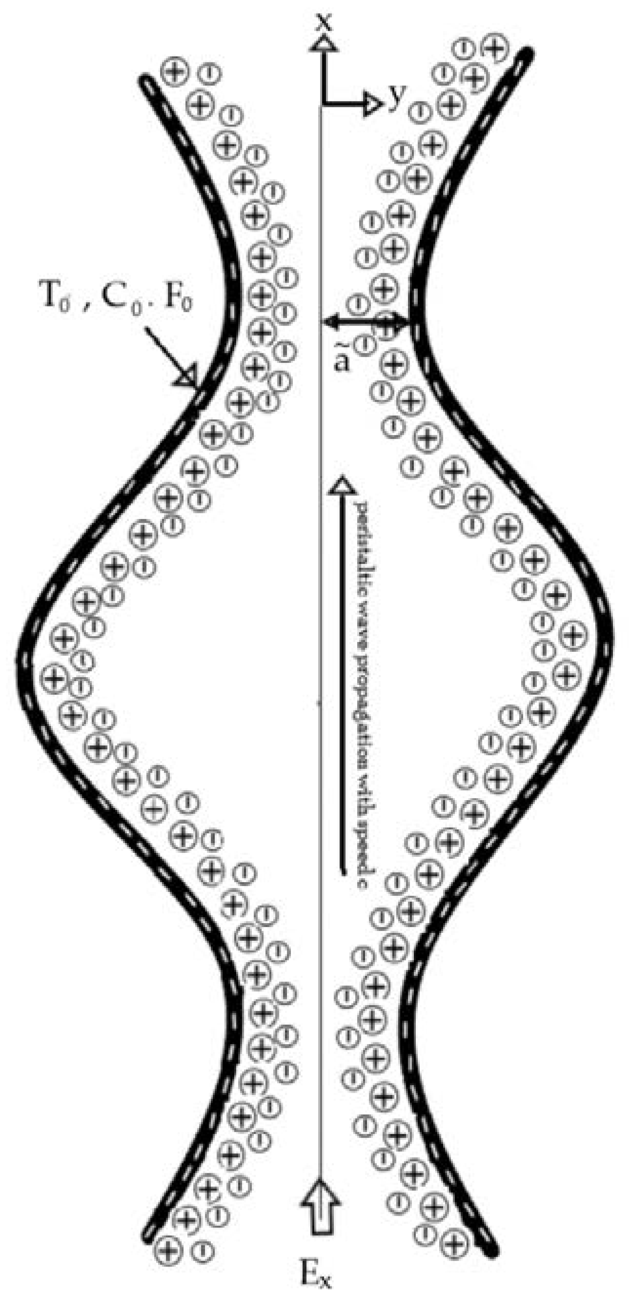
2.1. Flow Regime

The physical model (shown in Figure 1) consists of a two-dimensional EOF of nanofluid with double-diffusive convection through a microfluidic channel.

The medium is induced by propagating a peristaltic wave at velocity $c$ along the microchannel. The temperature, solutal concentration and nanoparticle fraction for the lower channel wall are taken as $T_0,C_0$ and $F_0$, respectively.

Mathematically, microchannel wall’s geometry is expressed as [23]

$$\tilde{h}\left(\tilde{X},\tilde{t}\right)=\tilde{a}+\tilde{b}\sin \left(2\pi \frac{\left(\tilde{X}-c\tilde{t}\right)}{\lambda }\right)$$

(1)

where $\tilde{h}$ represents the transverse vibration of the wall, $\tilde{a}$ is the half width of channel, $\tilde{b}$ is the amplitude of wave, $\tilde{X}$ represents the axial coordinate, $c$ is the speed of the wave,$\lambda$ represents the wavelength and $\tilde{t}$ is the time.

2.2. Governing Equations

The equations governing the physical flow problem for nanofluid with double-diffusive convection in electrohydrodynamic (EHD) are [19]

$$\frac{\partial \tilde{U}}{\partial \tilde{X}}+\frac{\partial \tilde{V}}{\partial \tilde{Y}}=0.$$

(2)

$${\rho }_f\left(\frac{\partial \tilde{U}}{\partial \tilde{t}}+\tilde{U}\frac{\partial \tilde{U}}{\partial \tilde{X}}+\tilde{V}\frac{\partial \tilde{U}}{\partial \tilde{Y}}\right)=-\frac{\partial \tilde{P}}{\partial \tilde{X}}+\mu \left(\frac{{\partial }^2\tilde{U}}{\partial {\tilde{X}}^2}+\frac{{\partial }^2\tilde{U}}{\partial {\tilde{Y}}^2}\right)+g\left\{\left(1-F_0\right){\rho }_0\left({\beta }_t\left(\tilde{T}-T_0\right)+ {\beta }_c\left(\tilde{C}-C_0\right)\right)-\left({\rho }_p-{\rho }_0\right)\left(\tilde{F}-F_0\right)\right\}+{\rho }_e{E}_x,$$

(3)

$${\rho }_f\left(\frac{\partial \tilde{V}}{\partial \tilde{t}}+\tilde{U}\frac{\partial \tilde{V}}{\partial \tilde{X}}+\tilde{V}\frac{\partial \tilde{V}}{\partial \tilde{Y}}\right)=-\frac{\partial \tilde{P}}{\partial \tilde{Y}}+\mu \left(\frac{{\partial }^2\tilde{V}}{\partial {\tilde{X}}^2}+\frac{{\partial }^2\tilde{V}}{\partial {\tilde{Y}}^2}\right)+g\left\{\left(1-F_0\right){\rho }_0\left({\beta }_t\left(\tilde{T}-T_0\right)+ {\beta }_c\left(\tilde{C}-C_0\right)\right)-\left({\rho }_p-{\rho }_0\right)\left(\tilde{F}-F_0\right)\right\}.$$

(4)

$${\left(\rho C_p\right)}_f\left(\frac{\partial \tilde{T}}{\partial \tilde{t}}+\tilde{U}\frac{\partial \tilde{T}}{\partial \tilde{X}}+\tilde{V}\frac{\partial \tilde{T}}{\partial \tilde{Y}}\right)=k\left(\frac{{\partial }^2\tilde{T}}{\partial {\tilde{X}}^2}+\frac{{\partial }^2\tilde{T}}{\partial {\tilde{Y}}^2}\right)+D_{tc}\left(\frac{{\partial }^2\tilde{C}}{\partial {\tilde{X}}^2}+\frac{{\partial }^2\tilde{C}}{\partial {\tilde{Y}}^2}\right)+{\left(\rho C_p\right)}_p\left\{D_b\right(\frac{\partial \tilde{F}\partial \tilde{T}}{\partial \tilde{X}\partial \tilde{X}}+\frac{\partial \tilde{F}\partial \tilde{T}}{\partial \tilde{Y}\partial \tilde{Y}})+\frac{D_t}{T_0}(({\frac{\partial \tilde{T}}{\partial \tilde{X}})}^2+{\left(\frac{\partial \tilde{T}}{\partial \tilde{Y}}\right)}^2)\}.$$

(5)

$$\left(\frac{\partial \tilde{C}}{\partial \tilde{t}}+\tilde{U}\frac{\partial \tilde{C}}{\partial \tilde{X}}+\tilde{V}\frac{\partial \tilde{C}}{\partial \tilde{Y}}\right)=D_s\left(\frac{{\partial }^2\tilde{C}}{\partial {\tilde{X}}^2}+\frac{{\partial }^2\tilde{C}}{\partial {\tilde{Y}}^2}\right)+D_{ct}\left(\frac{{\partial }^2\tilde{T}}{\partial {\tilde{X}}^2}+\frac{{\partial }^2\tilde{T}}{\partial {\tilde{Y}}^2}\right).$$

(6)

$$\left(\frac{\partial \tilde{F}}{\partial \tilde{t}}+\tilde{U}\frac{\partial \tilde{F}}{\partial \tilde{X}}+\tilde{V}\frac{\partial \tilde{F}}{\partial \tilde{Y}}\right)=D_b\left(\frac{{\partial }^2\tilde{F}}{\partial {\tilde{X}}^2}+\frac{{\partial }^2\tilde{F}}{\partial {\tilde{Y}}^2}\right)+\frac{D_t}{T_0}\left(\frac{{\partial }^2\tilde{T}}{\partial {\tilde{X}}^2}+\frac{{\partial }^2\tilde{T}}{\partial {\tilde{Y}}^2}\right).$$

(7)

Here,${\rho }_e$ is the electrical charge density, ${\rho }_f$ is the fluid density,${\rho }_p$ is the nanoparticle mass density, ${\rho }_0$ is the nanofluid density at reference temperature $\left(T_0\right), E_x$ is the applied electric field, $\tilde{U}$ represents the velocity along the $\tilde{X}$ direction, $\tilde{V}$ represents the velocity along the $\tilde{Y}$ direction, $\tilde{T}$ is the temperature, $\tilde{C}$ is the solutal concentration, $\tilde{F}$ is the nanoparticle volume fraction, $\tilde{P}$ is the pressure, $\mu$ is the fluid viscosity, $g$ is the acceleration due to gravity, ${\beta }_t$ is the volumetric thermal expansion coefficient of fluid, ${\beta }_c$ is the volumetric solutal expansion coefficient of fluid, ${(\rho c_p)}_f$ is the heat capacity of fluid, ${(\rho c_p)}_p$ is the effective heat capacity of nanoparticle, $k$ is the thermal conductivity, $D_{tc}$ is the Dufour diffusivity, $D_{ct}$ is the Soret diffusivity, $D_b$ is Brownian diffusion coefficient, $D_t$ is Thermophoretic diffusion coefficient and $D_s$ is solutal diffusivity.

The Poisson–Boltzmann equation [26] in a microchannel is defined as

$${\nabla }^2\tilde{\mathsf{\varphi }}=-\frac{{\rho }_e}{\in }.$$

(8)

Here, ${\rho }_e\left(=-z_{v}e\left({\tilde{n}}^{-}-{\tilde{n}}^{+}\right)\right)$ is the total charge density, $\in$ is the dielectric permittivity, $\tilde{\mathsf{\varphi }}$ is the electric potential, ${\tilde{n}}^{-}$ is the anion, ${\tilde{n}}^{+}$ is the cation and defined as ${\tilde{n}}^{\pm }={\tilde{n}}_0{e}^{\left(\pm \frac{e{z}_v}{T_{av}{K}_B}\tilde{\mathsf{\varphi }}\right)}$.

Moreover, $n_0,z_v,e,K_B$ and $T_{av}$ are the bulk concentration, charge balance, electronic charge, Boltzmann constant and average temperature, respectively.

The translational transformation between fixed coordinate system $\left(\tilde{X},\tilde{Y}\right)$ and moving coordinate system $\left(\tilde{x},\tilde{y}\right)$ is [8]

$$\begin{gathered} \tilde{x}=\tilde{X}-c\widetilde{t,}\tilde{y}=\tilde{Y},\tilde{u}\left(\tilde{x},\tilde{y}\right)=\tilde{U}\left(\tilde{X},\tilde{Y},\tilde{t}\right)-c,\tilde{v}\left(\tilde{x},\tilde{y}\right)=\tilde{V}\left(\tilde{X},\tilde{Y},\tilde{t}\right), \\ \tilde{p}\left(\tilde{x},\tilde{y}\right)=\tilde{P}\left(\tilde{X},\tilde{Y},\tilde{t}\right),T\left(\tilde{x},\tilde{y}\right)=\tilde{T}\left(\tilde{X},\tilde{Y},\tilde{t}\right). \end{gathered}$$

(9)

Using the transformations (9) in Equations (2)–(7), after introducing the dimensionless parameters:

$$\begin{gathered} x=\frac{\tilde{x}}{\lambda }, y=\frac{\tilde{y}}{\tilde{a}}, t=\frac{c\tilde{t}}{\lambda }, u=\frac{\tilde{u}}{c}, v=\frac{\tilde{v}}{\alpha c}, p=\frac{{\tilde{a}}^2}{\lambda c\mu }\tilde{p},\alpha =\frac{\tilde{a}}{\lambda }, h=\frac{\tilde{h}}{\tilde{a}}, n=\frac{\tilde{n}}{n_0},m_e=\frac{\tilde{a}}{{\lambda }_d},\mathsf{\epsilon }=\frac{\tilde{b}}{\tilde{a}}, \\ \theta =\frac{\tilde{T}-T_0}{T_0},\Omega =\frac{\tilde{C}-C_0}{C_0},\gamma =\frac{\tilde{F}-F_0}{F_0},{\lambda }_d{}^2=\frac{\in K_B{T}_0}{2n_0{\left(e{z}_v\right)}^2},\mathsf{\varphi }=\frac{e{z}_v}{T_{av}{K}_B}\tilde{\mathsf{\varphi }}, P_e=\frac{c\tilde{a}}{D}, R_e=\frac{{\rho }_{f}c\tilde{a} }{\mu }, \\ P_r=\frac{\mu {\left(\rho c_p\right)}_f}{{\rho }_{f}k}, U_{hs}=-\frac{T_{av}{K}_B{E}_x\in }{e{z}_{v}c\mu }, u=\frac{\partial \psi }{\partial y}, v=-\frac{\partial \psi }{\partial x}, G_{rt}=\frac{{\rho }_{0}g{\tilde{a}}^2{\beta }_t{T}_0\left(1-F_0\right)}{c\mu }, f=\frac{q}{c\tilde{a}}, \\ {G}_{rc}=\frac{{\rho }_{0}g{\tilde{a}}^2{\beta }_c{C}_0\left(1-F_0\right)}{c\mu }, G_{rf}=\frac{g{\tilde{a}}^2\left({\rho }_p-{\rho }_0\right)F_0}{c\mu }, N_t=\frac{D_t{(\rho c_p)}_p }{k}, S_s=\frac{c\tilde{a} }{D_s}, S_b=\frac{c\tilde{a} }{D_b}, \\ {N}_b=\frac{D_b{(\rho c_p)}_p{F}_0 }{k}, N_{ct}=\frac{D_{ct}{T}_0}{D_s{C}_0}, N_{tc}=\frac{D_{tc}{C}_0}{k{T}_0}, \end{gathered}$$

(10)

where $x,y,m_e,\alpha ,{\lambda }_d,p,U_{hs},\mathsf{\epsilon },\theta ,\Omega ,\gamma ,P_e,R_e,P_r,G_{rt},G_{rc},G_{rf},N_t,N_b,N_{ct},N_{tc},f$ and $\mathsf{\Theta }$ are non-dimensional axial coordinate, non-dimensional transverse coordinate, electro-osmotic parameter, peristaltic wave number, Debye length, non-dimensional pressure, Helmholtz-Smoluchowski velocity, amplitude ratio, dimensionless temperature, dimensionless species concentration, dimensionless nanoparticle volume fraction, ionic Peclet number, Reynolds number, Prandtl number, thermal Grashof number, solutal Grashof number, nanoparticle Grashof number, thermophoresis parameter, Brownian motion parameter, Soret parameter, Dufour parameter, dimensionless volume flow rate in moving frame and dimensionless volume flow rate in fixed frame, respectively.

Applying Debye-H$\ddot{\mathrm{u}}$ckel linearization approximation [27] and Equation (10), Equation (8) becomes

$$\frac{d^2\mathsf{\varphi }}{d{y}^2}=m_e{}^2\mathsf{\varphi },$$

(11)

where $m_e$ is the electro-osmotic parameter. The analytical solution of Equation (11) subject to boundary condition $\frac{\partial \mathsf{\varphi }}{\partial y}=0,$ at $y=0$ and $\mathsf{\varphi }=1,$ at $y=h\left(x\right)$ yeild

$$\mathsf{\varphi }\left(y\right)=\frac{\cosh \left(m_{e}y\right)}{\cosh \left(m_{e}h\right)}.$$

(12)

Using Equation (10), followed by long wavelength approximation [8], Equations (3)–(7) can be reduced to following form:

$$\frac{\partial p}{\partial x}=\frac{{\partial }^{2}u}{\partial y^2}+G_{rt}\theta +G_{rc}\Omega -G_{rf}\gamma +m_e{}^2{U}_{hs}\mathsf{\varphi },$$

(13)

$$\frac{\partial p}{\partial y}=0,$$

(14)

$$\frac{{\partial }^2\theta }{\partial y^2}+N_{tc}\frac{{\partial }^2\Omega }{\partial y^2}+N_b\frac{\partial \theta }{\partial y}\frac{\partial \gamma }{\partial y}+N_t{\left(\frac{\partial \theta }{\partial y}\right)}^2=0,$$

(15)

$$\frac{{\partial }^2\Omega }{\partial y^2}+N_{ct}\left(\frac{{\partial }^2\mathsf{\theta }}{\partial y^2}\right)=0,$$

(16)

$$\frac{{\partial }^2\gamma }{\partial y^2}+\frac{N_t}{N_b}\left(\frac{{\partial }^2\mathsf{\theta }}{\partial y^2}\right)=0.$$

(17)

The dimensionless boundary conditions are:

$$\frac{\partial u}{\partial y}=0, \theta =0, \Omega =0, \gamma =0, \mathrm{at}y=0,$$

(18a)

$$u=0, \theta =1, \Omega =1, \gamma =1,\mathrm{at}y=h\left(x\right)=1+\mathsf{\epsilon }\sin x,$$

(18b)

3. Solution Procedure

Analytical Solution

The analytical solutions [17] of temperature, solutal concentration and nanoparticle volume fraction field are obtained after solving simultaneous Equations (15)–(17) subject to boundary condition (18a,b):

$$\theta =\frac{e^{-N_{0}y}-1}{e^{-N_{0}h}-1},$$

(19)

$$\Omega =\frac{N_t}{N_b}\left(\frac{e^{-N_{0}y}-1}{1- e^{-N_{0}h}}\right)+\frac{1}{h}\left(1+\frac{N_t}{N_b}\right)y,$$

(20)

$$\gamma =N_{ct}\left(\frac{e^{-N_{0}y}-1}{1- e^{-N_{0}h}}\right)+\frac{1}{h}\left(1+N_{ct}\right)y.$$

(21)

Using Equations (19)–(21) in Equation (13) and using boundary condition (18a) and (18b), the analytical solution of axial velocity is obtained as:

$$u=\frac{1}{2}\frac{\partial p}{\partial x}\left(y^2-h^2\right)-N_1\left\{\frac{1}{2}\left(y^2-h^2\right)-\frac{1}{N_0{}^2}\left(e^{-N_{0}y}-e^{-N_{0}h}\right)-\frac{1}{N_0}\left(y-h\right)\right\}-\frac{N_2}{6}\left(y^3-h^3\right)+ U_{hs}\left(1-\frac{\cosh \left(m_{e}y\right)}{\cosh \left(m_{e}h\right)}\right),$$

(22)

where

$$\begin{gathered} N_0=\frac{1}{h}\left(\frac{N_t+N_b}{1-N_{ct}{N}_{tc}}\right), \\ {N}_1=\frac{1}{1- e^{-N_{0}h}}\left(G_{rt}-G_{rc}\Omega N_{ct}+\frac{N_t}{N_b}{G}_{rf}\right), \\ {N}_2=\frac{1}{h}\left(G_{rc}\left(1+N_{ct}\right)-\left(1+\frac{N_t}{N_b}\right)G_{rf}\right). \end{gathered}$$

The volume flow rate is given by

$$Q={{\displaystyle \int }}_0^{h}udy,$$

(23)

Using Equation (22) after rearranging the terms, pressure gradient is obtained as

$$\frac{\partial p}{\partial x}=\frac{-3Q}{h^3}-N_1\left\{\frac{3e^{-N_{0}h}}{N_0{}^3{h}^3}\left(1+N_{0}h\right)-\frac{3}{N_0{}^3{h}^3}+\frac{3}{2N_{0}h}-1\right\}+\frac{3N_2}{8}h+\frac{3U_{hs}}{h^3}\left(h-\frac{\sinh \left(m_{e}h\right)}{m_e\cosh \left(m_{e}h\right)}\right).$$

(24)

The pressure rise across one wavelength $\mathsf{\Delta }P$ is as follows:

$$\mathsf{\Delta }P={{\displaystyle \int }}_0^1\frac{\partial p}{\partial x}dx.$$

(25)

The volume flow rate in fixed frame is given by

$$Q={{\displaystyle \int }}_0^h\tilde{U}\left(\tilde{X},\tilde{Y},\tilde{t}\right)d\tilde{Y}.$$

(26)

Using Equation (9) in Equation (26) and after integration, we obtain

$$Q=q+ch.$$

(27)

The time average flow rate over one time period is defined as

$$\tilde{Q}={{\displaystyle \int }}_0^{1}Qdt.$$

(28)

Using Equations (10) and (27) in Equation (28), we obtain

$$\mathsf{\Theta }=f+1.$$

(29)

The stream function $\left(u=\frac{\partial \psi }{\partial y}, v=-\frac{\partial \psi }{\partial x}\right)$ in wave frame takes the following form:

$$\psi =\frac{1}{2}\frac{\partial p}{\partial x}\left(\frac{1}{3}{y}^3-h^{2}y\right)-N_1\left\{\frac{1}{2}\left(\frac{1}{3}{y}^3-h^{2}y\right)+\frac{1}{N_0{}^2}\left(\frac{1}{N_0}{e}^{-N_{0}y}+y{e}^{-N_{0}h}+\frac{1}{N_0}\right)-\frac{1}{N_0}\left(\frac{1}{2}{y}^2-hy\right)\right\}-\frac{N_2}{6}\left(\frac{1}{4}{y}^4-y{h}^3\right)-y+U_{hs}\left(y-\frac{\sinh \left(m_{e}h\right)}{m_e\cosh \left(m_{e}h\right)}\right).$$

(30)

The heat transfer coefficient $Z$ at the wall ($y=h\left(x\right)$) is as follows:

$$Z=h_x\frac{\partial \theta }{\partial y}{|}_{y=h}.$$

(31)

4. Entropy Generation Analysis

The dimensional volumetric entropy generation during nanofluid flow with double diffusive convection is given by

$$S_{gen}=\frac{k}{{\tilde{T}}^2}({(\frac{\partial \tilde{T}}{\partial \tilde{X}})}^2+{(\frac{\partial \tilde{T}}{\partial \tilde{Y}})}^2))+[\frac{D_{tc}}{\tilde{T}}(\frac{{\partial }^2}{\partial {\tilde{X}}^2}+\frac{{\partial }^2}{\partial {\tilde{Y}}^2})\tilde{C}+\frac{{\left(\rho C_p\right)}_p}{\tilde{T}}\{D_b(\frac{\partial \tilde{F}\partial \tilde{T}}{\partial \tilde{X}\partial \tilde{X}}+\frac{\partial \tilde{F}\partial \tilde{T}}{\partial \tilde{Y}\partial \tilde{Y}})+\frac{D_t}{T_0}(({\frac{\partial \tilde{T}}{\partial \tilde{X}})}^2+{(\frac{\partial \tilde{T}}{\partial \tilde{Y}})}^2)\}]$$

(32)

Equation (32) comprises two parts: one part consists of entropy generation due to heat transfer and the second part consists of entropy generation due to solutal concentration.

The characteristics entropy generation is given as

$$S_g=\frac{k}{{\tilde{a}}^2}.$$

(33)

Using Equations (10) and (33), the non-dimensional volumetric entropy generation can be expressed as

$$N_s=\frac{S_{gen}}{S_g}=\frac{1}{{\left(1+\theta \right)}^2}\frac{{\partial }^2\theta }{\partial y^2}+\frac{1}{1+\theta }\left[N_{tc}\frac{{\partial }^2\Omega }{\partial y^2}+N_b\frac{\partial \theta }{\partial y}\frac{\partial \gamma }{\partial y}+N_t{\left(\frac{\partial \theta }{\partial y}\right)}^2\right],$$

(34)

The total entropy generation or entropy generation number $N_s$ in Equation (34) can be written as sum of

$$N_s=N_{HT}+N_{DC}.$$

(35)

Here, $N_{HT}$ is the dimensionless entropy generation due to heat transfer and $N_{DC}$ represent the dimensionless entropy generation due to solutal concentration.

The thermal irreversibility of the system is defined as the Bejan number $B_e$ [38]:

$$B_e=\frac{N_{HT}}{N_{HT}+N_{DC}}=\frac{N_{HT}}{N_s}=\frac{\frac{1}{{\left(1+\theta \right)}^2}\frac{{\partial }^2\theta }{\partial y^2}}{\frac{1}{{\left(1+\theta \right)}^2}\frac{{\partial }^2\theta }{\partial y^2}+\frac{1}{1+\theta }\left[N_{tc}\frac{{\partial }^2\Omega }{\partial y^2}+N_b\frac{\partial \theta }{\partial y}\frac{\partial \gamma }{\partial y}+N_t{\left(\frac{\partial \theta }{\partial y}\right)}^2\right]}.$$

(36)

5. Results and Discussion

The main objective of this section is to explain the effects of various parameters (i.e., thermophoresis parameter $N_t$, Brownian motion parameter $N_b$, Soret parameter $N_{ct}$, Dufour parameter $N_{tc}$, thermal Grashof number $G_{rt}$, solutal Grashof number $G_{rc}$, nanoparticle Grashof number $G_{rf}$, electro-osmotic parameter $m_e$ and Helmholtz-Smoluchowski velocity $U_{hs}$) on the velocity profile $u$, pressure rise $\mathsf{\Delta }P$, pressure gradient $dp/dx$, temperature profile $\theta$, solutal concentration profile $\Omega$, nanoparticle volume faction profile $\gamma$_, entropy generation number $N_s$, Bejan number $B_e$ and heat transfer coefficient $Z$. Moreover, the trapping phenomenon is also illustrated. The graphical results are shown in Figure 2, Figure 3, Figure 4, Figure 5, Figure 6, Figure 7, Figure 8, Figure 9, Figure 10, Figure 11, Figure 12, Figure 13, Figure 14, Figure 15, Figure 16 and Figure 17.

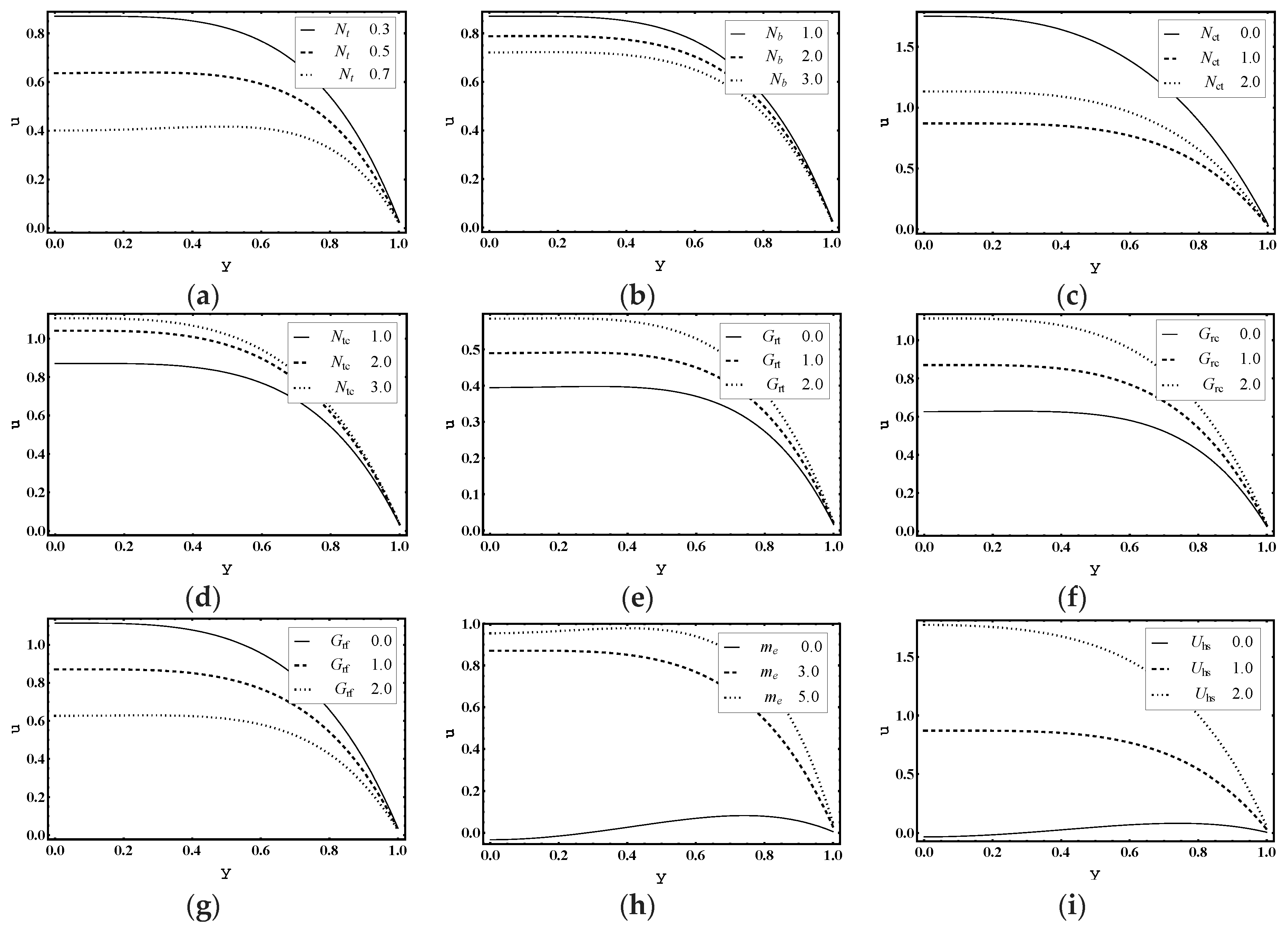
5.1. Flow Characteristics

Figure 2a–i is displayed to show the advancements of physical parameters in velocity across the microchannel. Figure 2a,b shows that the magnitude of axial velocity $u$ decreased for increasing values of $N_t$ and $N_b$. As a result, the deposition of thermophoretic particles was reduced and the central axes of the micro channel had an increased particle accumulation. This sedimentation of the nanoparticles can be adjusted by controlling the thermal gradient, applied externally to the fluid. This is significant as nanoparticle suspension in the nanofluid blocks the fluid flow which affects the system’s performance. Consequently, monitoring the deposition of nanoparticles in the fluid is the main requirement. Figure 2c demonstrates that the magnitude of $u$ was reduced for increasing values of $N_{ct}$, although in Figure 2d, a contrary response is observed for $N_{tc}$. Figure 2e,f portrays that the magnitude of $u$ increased with the increase in $G_{rt}$ and $G_{rc}$. However, it declined for increasing values of $G_{rf}$, as shown in Figure 2g. This demonstrates that the change in concentration of nanoparticles reduced velocity while with a changing temperature and solutal concentration, velocity progresses. Figure 2h predicts that $m_e$ will enhance the magnitude of axial velocity $u$. Since $m_e$ is the ratio of the channel height to the Debye length ${\lambda }_d$, it indicates that ${\lambda }_d$ is inversely proportional to electric double layer thickness. Hence, more fluid flows in the central region. Figure 2i visualizes that $U_{hs}$ develops the magnitude of $u$. That means velocity of the fluid can be improved by increasing the magnitude of external electric field.

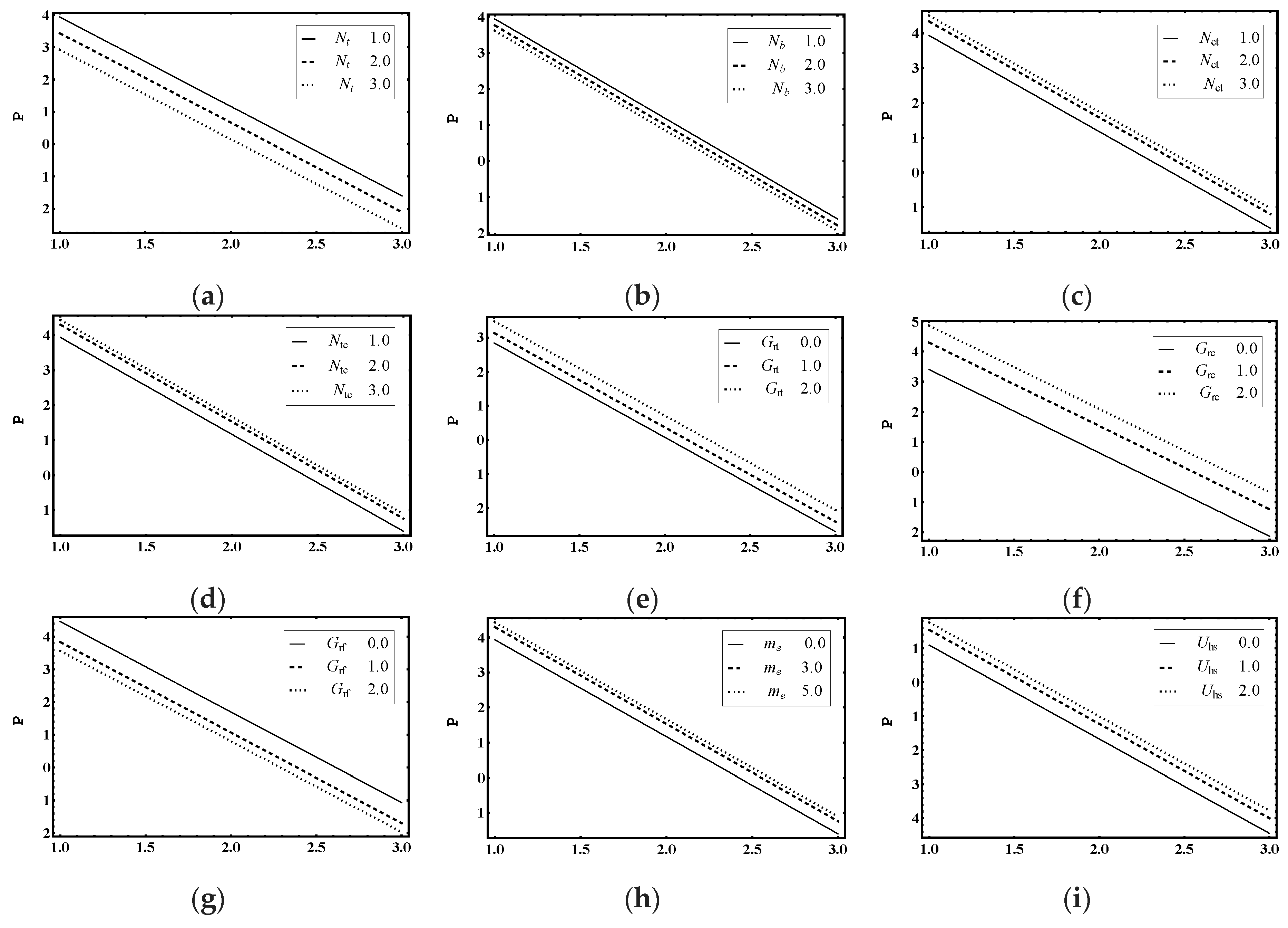
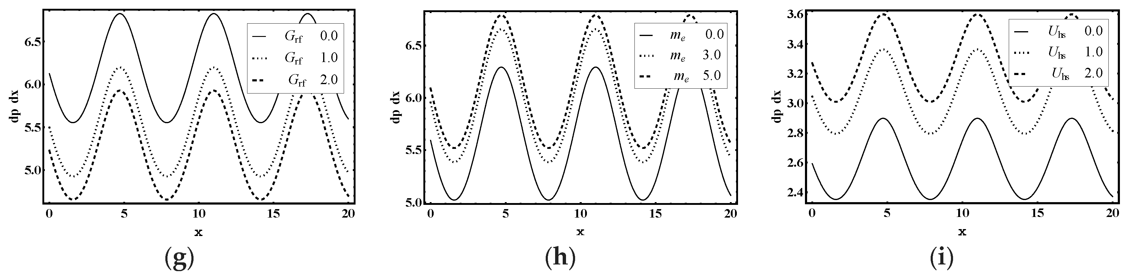
5.2. Pumping Characteristics

Figure 3a–i shows the variation of pressure difference across one wavelength $\mathsf{\Delta }P$ against the average flow rate $\mathsf{\Theta }$. These figures show the linear relationship between $\mathsf{\Delta }P$ and $\mathsf{\Theta }$. The pumping phenomenon was divided into four segments: pumping region (adverse pressure gradient $\mathsf{\Delta }P>0$, Positive pumping $\mathsf{\Theta }>0$), backward/retrograde pumping ($\mathsf{\Delta }P>0$,$\mathsf{\Theta }<0$), augmented pumping (favorable pressure gradient $\mathsf{\Delta }P<0$, Positive pumping $\mathsf{\Theta }>0$) and free pumping ($\mathsf{\Delta }P=0$). Figure 3a,b represents $\mathsf{\Delta }P$ for increasing values of $N_t$ and $N_b$. This shows that pumping decreased throughout the whole region. This is very helpful in nanofluid drug delivery systems [11]. Figure 3c–i highlights that pumping increased as the Soret parameter $N_{ct}$, the Dufour parameter $N_{tc}$, the thermal Grashof number $G_{rt}$, the solutal Grashof number $G_{rc}$, the nanoparticle Grashof number $G_{rf}$, the electro-osmotic parameter $m_e$ and Helmholtz–Smoluchowski velocity $U_{hs}$ increased. Here, $\mathsf{\Delta }P$ is in a linear relationship with flow rate $\mathsf{\Theta }$.

The variation of pressure gradient $dp/dx$ is presented in Figure 4a–i for different physical flow parameters. Figure 4a,b highlights that the magnitude of $dp/dx$ decreased as $N_t$ and $N_b$ increased. Figure 4c–f shows that the Soret parameter $N_{ct}$, the Dufour parameter $N_{tc}$, the thermal Grashof number $G_{rt}$ and the solutal Grashof number $G_{rc}$ distinctly enhanced the magnitude of $dp/dx.$ Conversely, nanoparticle Grashof number $G_{rf}$ acted to strongly reduce $dp/dx$ values, as shown in Figure 4g. This demonstrates that $dp/dx$ can be controlled by adjusting the $G_{rf}$. However, Figure 4h,i shows that the values of $dp/dx$ were enhanced for increasing values of electro-osmotic parameter $m_e$ and the Helmholtz–Smoluchowski velocity $U_{hs}$.

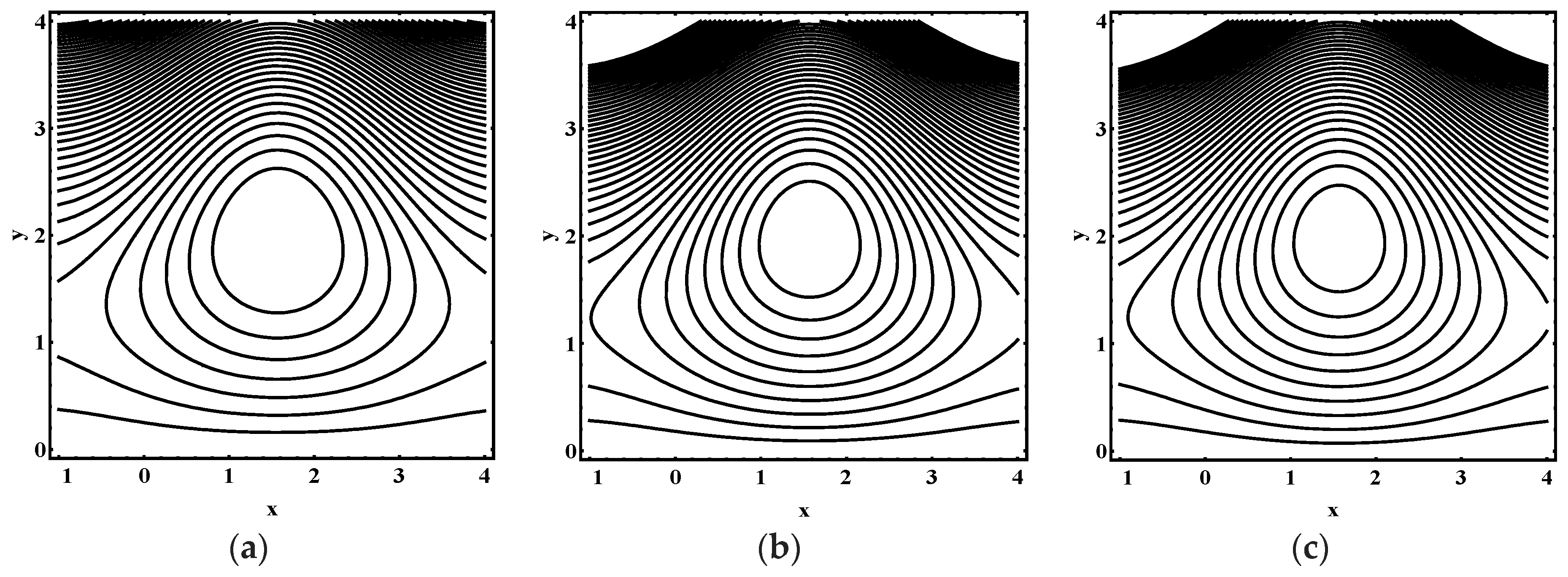
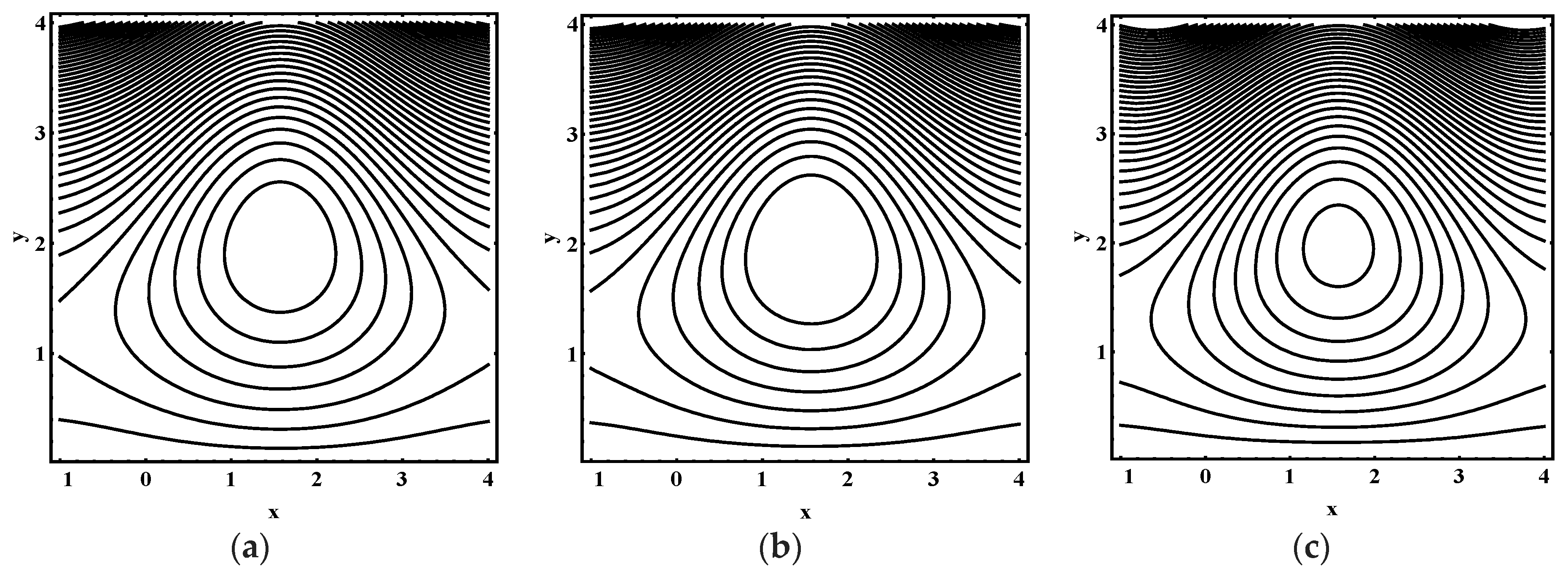
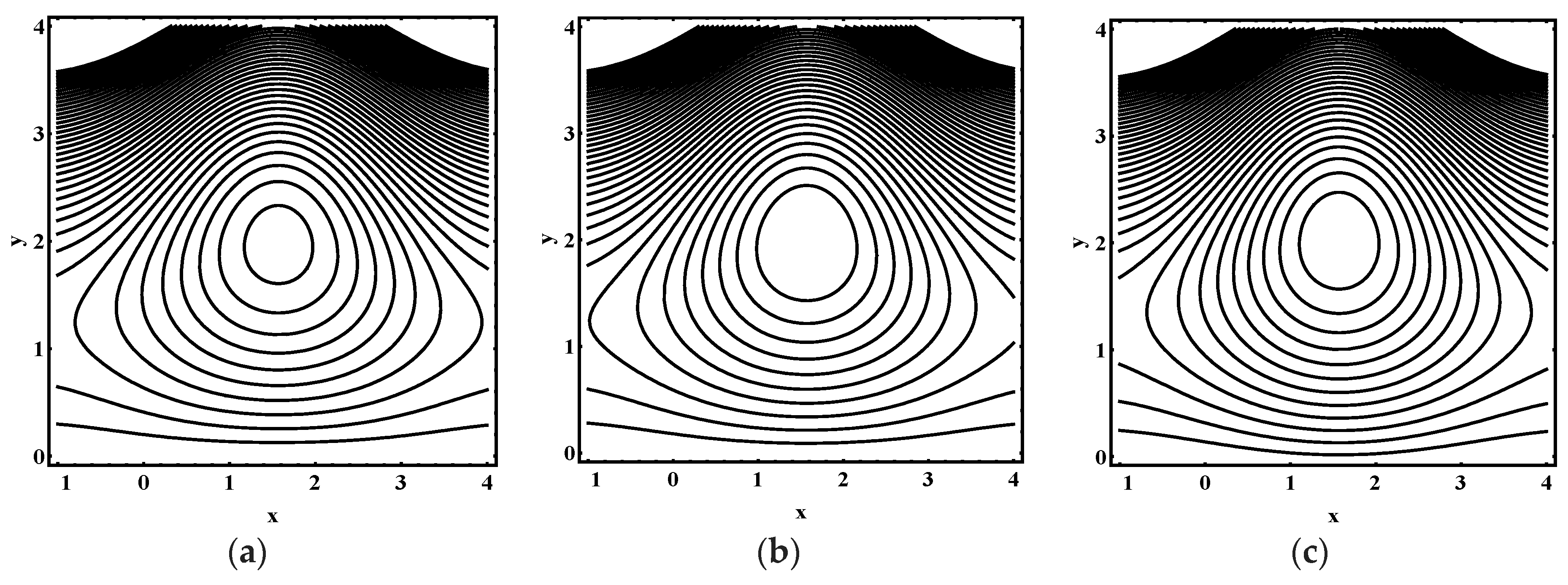
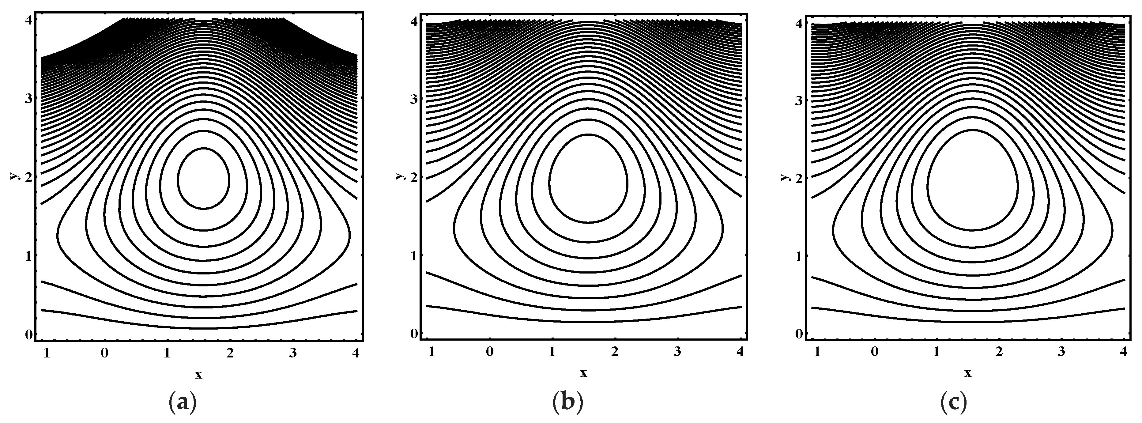
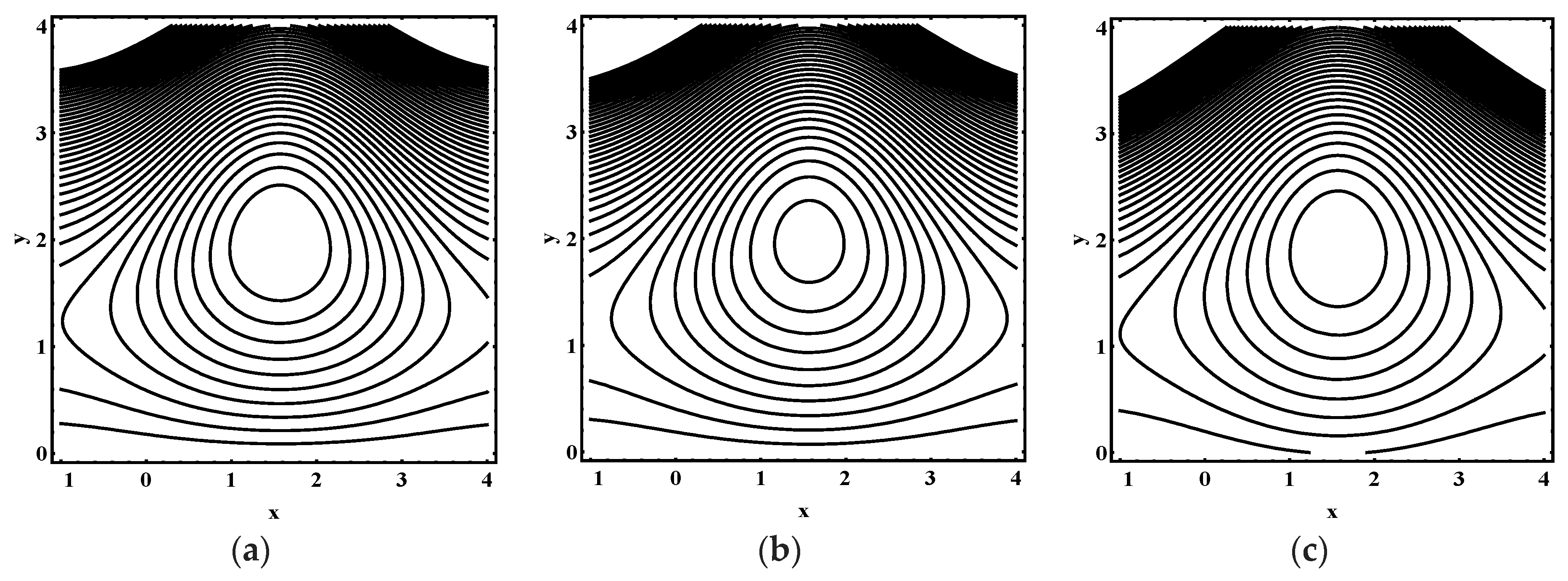
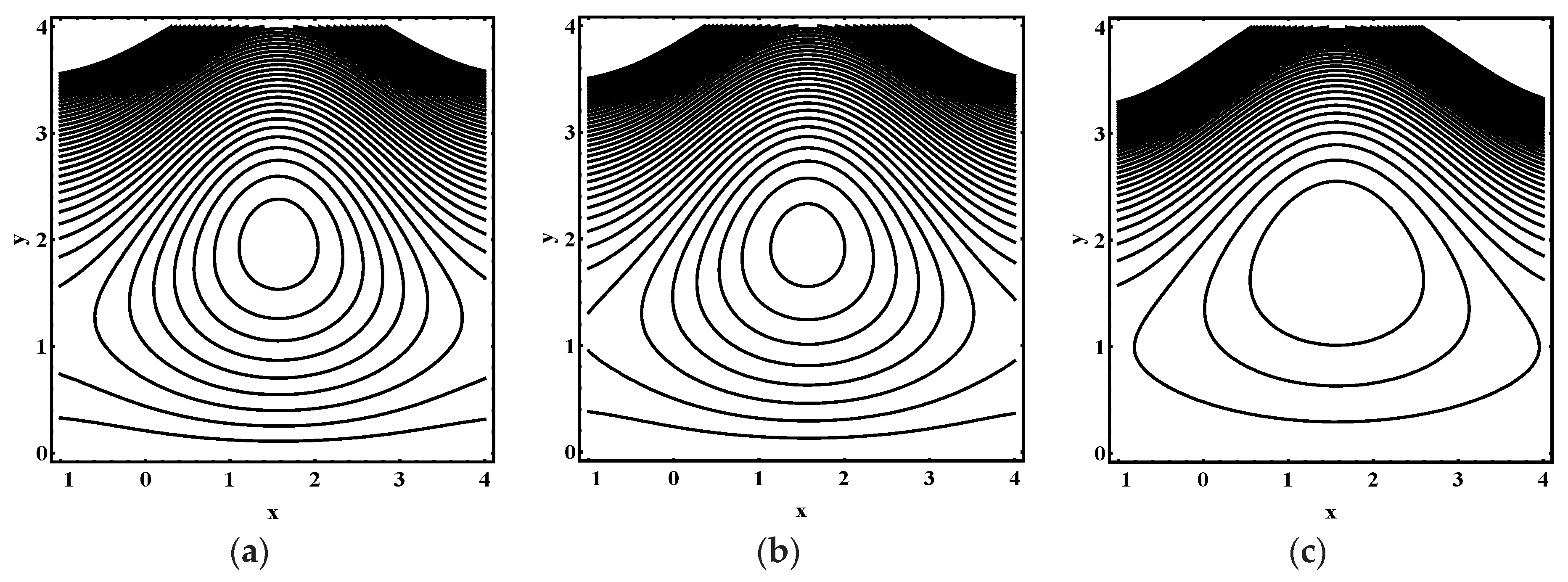
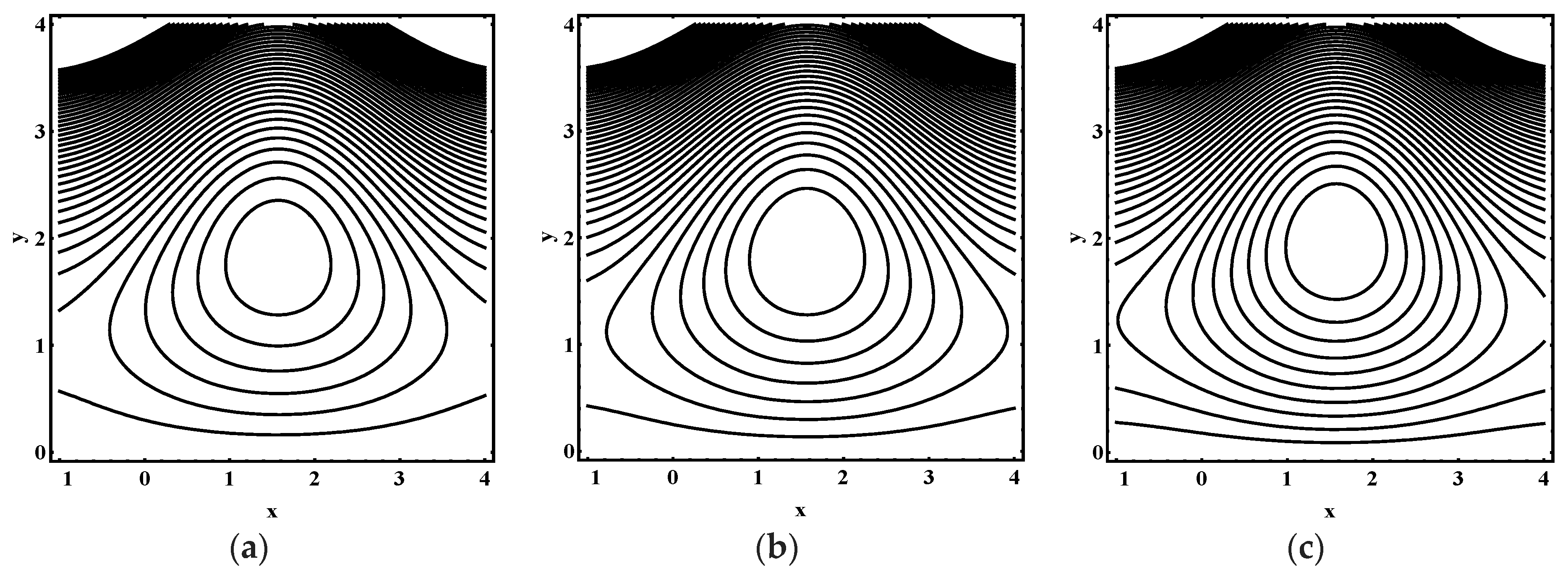
5.3. Trapping Characteristics

Trapping for different values of the thermophoresis parameter $N_t$, Brownian motion parameter $N_b$, Soret parameter $N_{ct}$, Dufour parameter $N_{tc}$, thermal Grashof number $G_{rt}$, solutal Grashof number $G_{rc}$, nanoparticle Grashof number $G_{rf}$, electro-osmotic parameter $m_e$ and Helmholtz-Smoluchowski velocity $U_{hs}$ are shown in Figure 5, Figure 6, Figure 7, Figure 8, Figure 9, Figure 10 and Figure 11. Figure 5a–c and Figure 6a–c display streamline structure for different values of $N_t$ and $N_b$. These reveal that the number and size of trapped bolus increased as $N_t$ and N_b increases. Figure 7a–c shows that the size of trapped bolus expanded with increasing $G_{rt}$. However, a reverse trend for solutal Grashof number $G_{rc}$, nanoparticle Grashof number $G_{rf}$ and electro-osmotic parameter $m_e$ (shown in Figure 8, Figure 9 and Figure 10). Furthermore, Figure 11a–c discloses that the number of trapped bolus increased for dissimilar values of $U_{hs}$.

5.4. Temperature Characteristics

The effects of thermophoresis parameter $N_t$, Brownian motion parameter $N_b$, Soret parameter $N_{ct}$ and Dufour parameter $N_{tc}$ were examined for heat profile $\theta$. Figure 12a,b demonstrates that the magnitude of temperature distribution $\theta$ declines for values of $N_t$ and $N_b.$ In addition, Figure 12c displays that the magnitude of temperature distribution $\theta$ was enhanced for more values of $N_{ct}.$ As, Soret parameter $N_{ct}$ is the ratio of temperature to concentration, hence, bigger $N_{ct}$ stands for a higher temperature. Figure 12d shows that the magnitude of temperature distribution $\theta$ was boosted for higher values of $N_{tc}.$ Since $N_{tc}$ shows the contribution of concentration gradient to thermal energy flux in the flow, it is evident that the increase in $N_{tc}$ caused a rise in temperature.

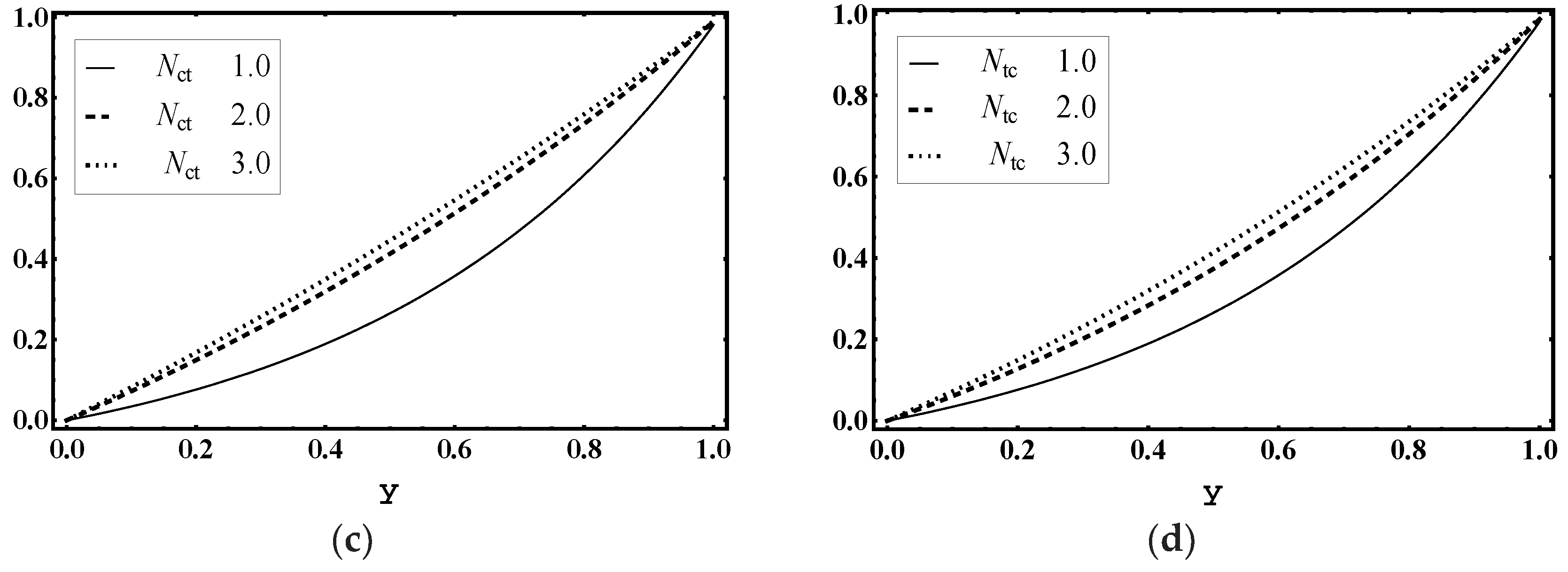
5.5. Concentration Characteristics

The influence of thermophoresis parameter $N_t$, Brownian motion parameter $N_b$, Soret parameter $N_{ct}$ and Dufour parameter $N_{tc}$ are observed for concentration profile $\Omega$. Figure 13a,b concludes that the magnitude of $\Omega$ increased for more values of $N_t$ and $N_b.$ Moreover, Figure 13c displays that the magnitude of $\Omega$ decayed for more values of $N_{ct}.$ In addition, Soret parameter $N_{ct}$ is the ratio of temperature to concentration. Hence, higher values of $N_{ct}$ lead to decay in concentration. Figure 13d shows that the magnitude of $\Omega$ declined for higher values of $N_{tc}.$

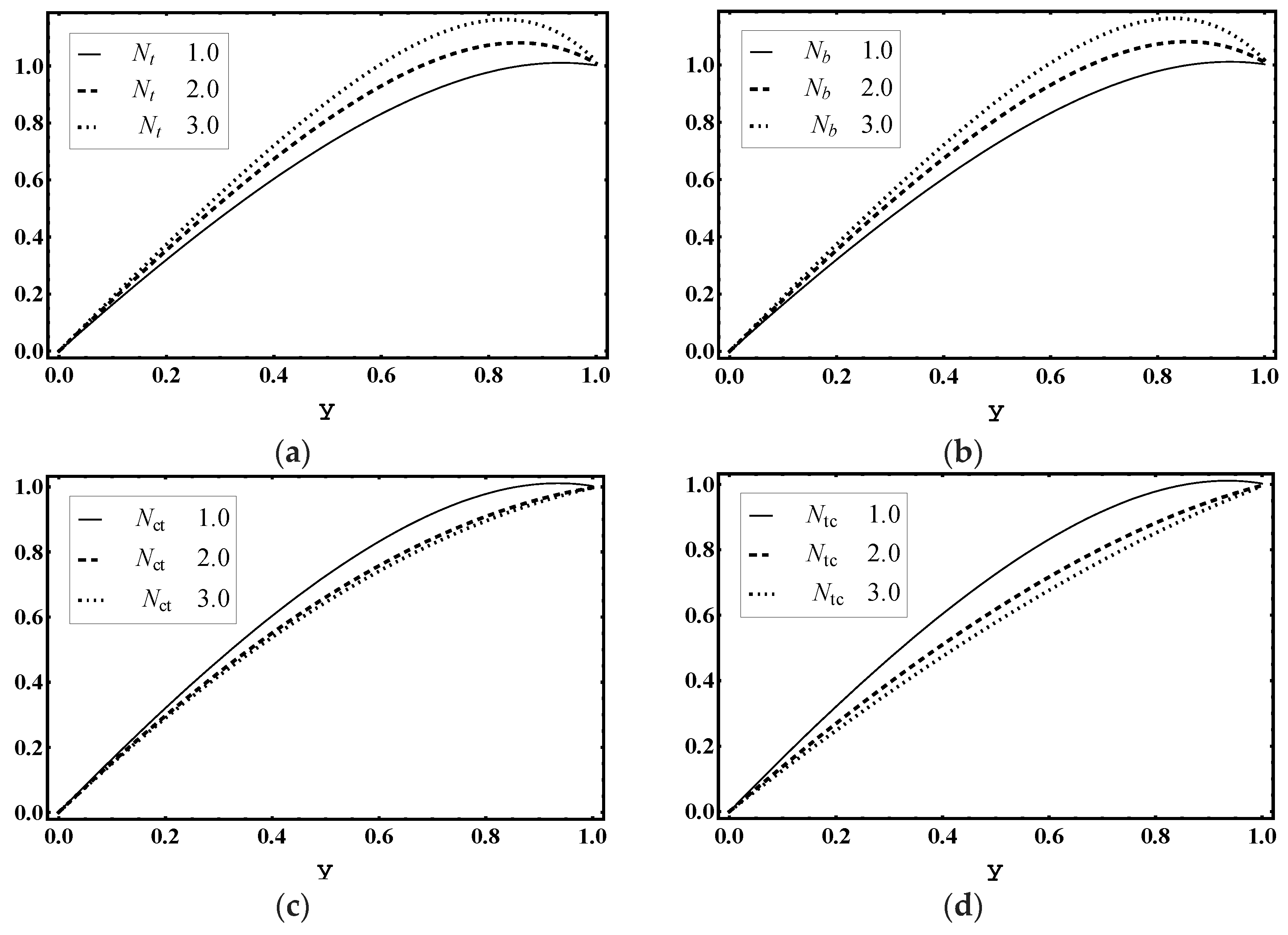
5.6. Nanoparticle Volume Fraction Characteristics

The influence of thermophoresis parameter $N_t$, Brownian motion parameter $N_b$, Soret parameter $N_{ct}$ and Dufour parameter $N_{tc}$ is noticed for nanoparticle volume fraction profile $\gamma$. Figure 14a demonstrates that the magnitude of $\gamma$ increased for more values of $N_t$. However, Figure 14b–d shows that the magnitude of $\gamma$ declined for higher values of Brownian motion parameter $N_b$, Soret parameter $N_{ct}$ and Dufour parameter $N_{tc}$.

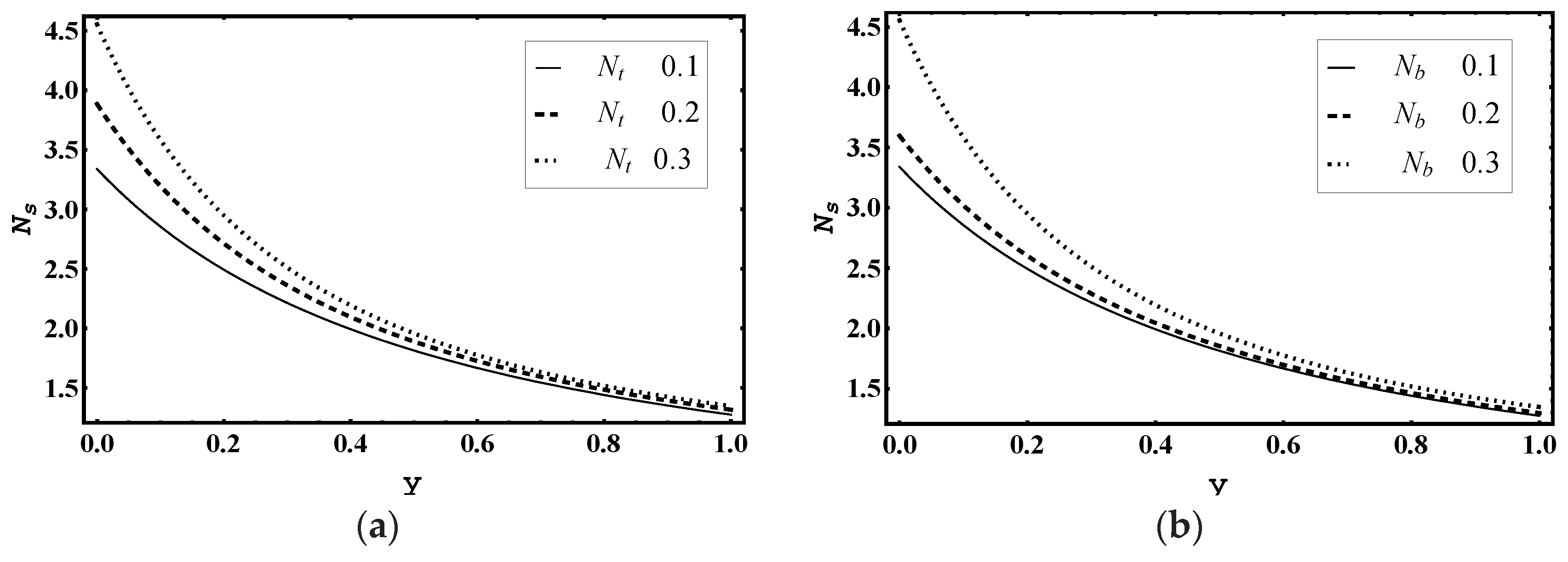
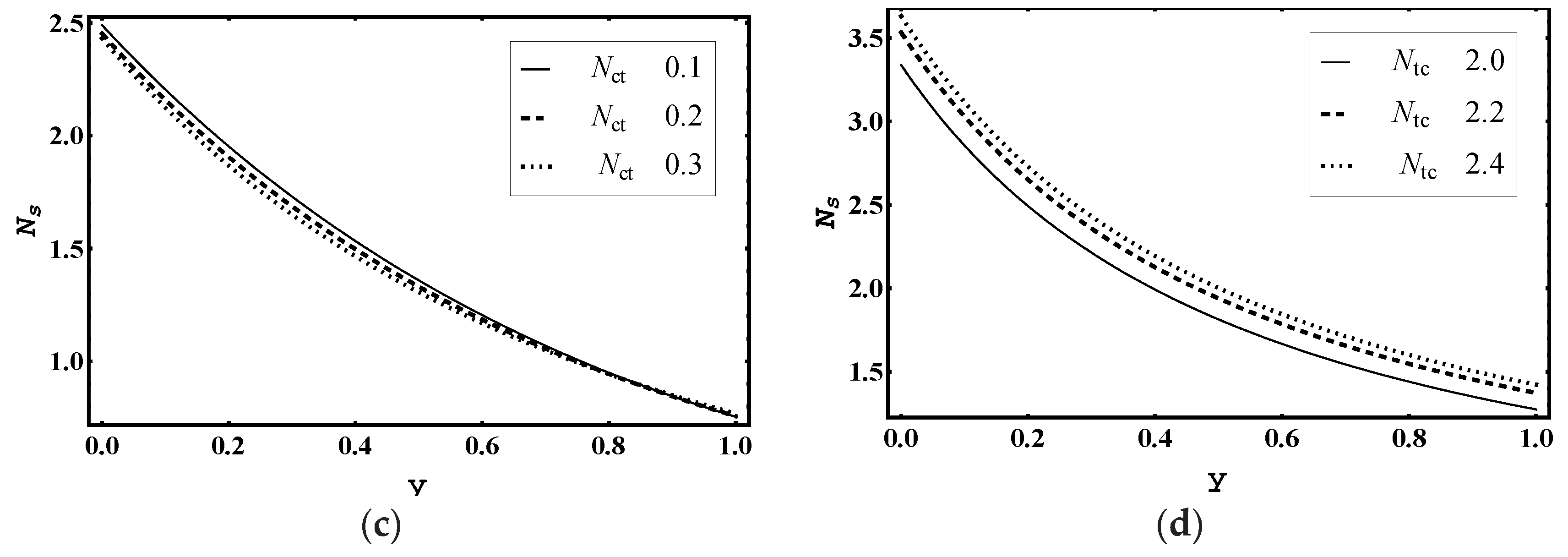
5.7. Entropy Production

Figure 15a–d illustrates the impact of thermophoresis parameter $N_t$, Brownian motion parameter $N_b$, Soret parameter $N_{ct}$ and Dufour parameter $N_{tc}$ on entropy generation number $N_s$. Figure 15a,b demonstrates that the magnitude of $N_s$ increased for added values of $N_t$ and $N_b.$ This was due to thermal irreversibility, i.e., for higher value of $N_t$ and $N_b,$ thermal irreversibility increased very quickly, near the wall. Moreover, Figure 15c displays that the magnitude of $N_s$ decayed for more values of $N_{ct}.$ Figure 15d shows that the magnitude of $N_s$ increased for higher values of $N_{tc}.$

Figure 16a–d demonstrates the effect of thermophoresis parameter $N_t$, Brownian motion parameter $N_b$, Soret parameter $N_{ct}$ and Dufour parameter $N_{tc}$ on Bejan number $B_e$. Figure 16a,b implies that the magnitude of $B_e$ declined for more values of $N_t$ and $N_b.$ In addition, Figure 16c displays that the magnitude of $B_e$ enhanced for more values of $N_{ct}$ near $y=0$. Figure 16d shows that the magnitude of $N_s$ ascended near $y=0$ for higher values of $N_{tc}$.

5.8. Heat Transfer Coefficient

Figure 17a–d reveals the changes in heat transfer coefficient $Z$ for different values of thermophoresis parameter $N_t$, Brownian motion parameter $N_b$, Soret parameter $N_{ct}$ and Dufour parameter $N_{tc}$. This infers that for various values of $N_t$ and $N_b$, the magnitude of heat transfer coefficient $Z$ increased. However, the magnitude of heat transfer coefficient $Z$ declined for bigger values of $N_{ct}$ and $N_{tc}$, respectively.

6. Concluding Remarks

A theoretical model for the entropy generation in electro-osmotic peristaltic flow of nanofluid with double-diffusive convection through microchannel is reported. The exact solutions are presented for quantities of interest. The results of this study are similar to the results of [11], when $U_{hs}=0$. Moreover, results of this study are comparable to the results of [6], when $G_{rt}=G_{rc}=G_{rf}=U_{hs}=0$. From the current analysis, we conclude that

• The magnitude of total entropy generation increased as the thermophoresis parameter and Brownian motion parameter increases.
• Soret parameter and Dufour parameter $N_{tc}$ strongly controlld the temperature profile and Bejan number profile.
• The velocity, pressure difference, pressure rise, temperature and Bejan number profile decreased as thermophoresis parameter and Brownian motion parameter increased.
• Electro-osmotic parameter strongly affected the velocity profile.
• The magnitude of pressure difference and pressure gradient enhances in the pumping region with the increase in Soret parameter, Dufour parameter, thermal Grashof number, solutal Grashof number, nanoparticle Grashof number, electro-osmotic parameter and Helmholtz-Smoluchowski velocity.
• The volume and number of trapped bolus increased as the thermophoresis parameter $N_t$, Brownian motion parameter, thermal Grashof number and Helmholtz-Smoluchowski velocity increases.
• Heat transfer coefficient, entropy generation number and nanoparticles volume fraction strongly surged with the thermophoresis parameter and the Brownian motion parameter increased.

References

1. Reuss, F.F. Charge-induced flow. Proc. Imp. Soc. Nat. Mosc. 1809, 3, 327–344. [Google Scholar]
2. Patankar, N.A.; Hu, H.H. Numerical simulation of electroosmotic flow. Anal. Chem. 1998, 70, 1870–1881. [Google Scholar] [CrossRef]
3. Yang, R.J.; Fu, L.M.; Lin, Y.C. Electroosmotic flow in microchannels. J. Colloid Interface Sci. 2001, 239, 98–105. [Google Scholar] [CrossRef] [PubMed]
4. Tang, G.H.; Li, X.F.; He, Y.L.; Tao, W.Q. Electroosmotic flow of non-Newtonian fluid in microchannels. J. Non-Newton. Fluid Mech. 2009, 157, 133–137. [Google Scholar] [CrossRef]
5. Miller, S.A.; Young, V.Y.; Martin, C.R. Electroosmotic flow in template-prepared carbon nanotube membranes. J. Am. Chem. Soc. 2001, 123, 12335–12342. [Google Scholar] [CrossRef] [PubMed]
6. Shapiro, A.H.; Jaffrin, M.Y.; Weinberg, S.L. Peristaltic pumping with long wavelengths at low Reynolds number. J. Fluid Mech. 1969, 37, 799–825. [Google Scholar] [CrossRef]
7. Noreen, S.; Qasim, M. Peristaltic flow with inclined magnetic field and convective boundary conditions. Appl. Bionics Biomech. 2014, 11, 61–67. [Google Scholar] [CrossRef]
8. Noreen, S.; Qasim, M. Influence of Hall Current and Viscous Dissipation on Pressure Driven Flow of Pseudoplastic Fluid with Heat Generation: A Mathematical Study. PLoS ONE 2015, 10, e0129588. [Google Scholar] [CrossRef] [PubMed]
9. Kefayati, G.R. Magnetic field effect on heat and mass transfer of mixed convection of shear-thinning fluids in a lid-driven enclosure with non-uniform boundary conditions. J. Taiwan Inst. Chem. Eng. 2015, 51, 20–33. [Google Scholar] [CrossRef]
10. Noreen, S. Effects of Joule Heating and Convective Boundary Conditions on Magnetohydrodynamic Peristaltic Flow of Couple-Stress Fluid. J. Heat Transf. 2016, 138, 094502. [Google Scholar] [CrossRef]
11. Noreen, S. Magneto-thermo hydrodynamic peristaltic flow of Eyring-Powell nanofluid in asymmetric channel. Nonlinear Eng. 2018, 7, 83–90. [Google Scholar] [CrossRef]
12. Akbar, N.S.; Nadeem, S. Endoscopic effects on peristaltic flow of a nanofluid. Commun. Theor. Phys. 2011, 56, 761. [Google Scholar] [CrossRef]
13. Noreen, S. Mixed convection peristaltic flow of third order nanofluid with an induced magnetic field. PLoS ONE 2013, 8, e78770. [Google Scholar] [CrossRef] [PubMed]
14. Tripathi, D.; Bég, O.A. A study on peristaltic flow of nanofluids: Application in drug delivery systems. Int. J. Heat Mass Transf. 2014, 70, 61–70. [Google Scholar] [CrossRef]
15. Reddy, M.G.; Reddy, K.V. Influence of Joule heating on MHD peristaltic flow of a nanofluid with compliant walls. Procedia Eng. 2015, 127, 1002–1009. [Google Scholar] [CrossRef]
16. Ebaid, A.; Aly, E.H. Additional results for the peristaltic transport of viscous nanofluid in an asymmetric channel with effects of the convective conditions. Natl. Acad. Sci. Lett. 2018, 41, 59–63. [Google Scholar] [CrossRef]
17. Shao, Q.; Fahs, M.; Younes, A.; Makradi, A.; Mara, T. A new benchmark reference solution for double-diffusive convection in a heterogeneous porous medium. Numer. Heat Transf. Part B Fundam. 2016, 70, 373–392. [Google Scholar] [CrossRef]
18. Huppert, H.E.; Turner, J.S. Double-diffusive convection. J. Fluid Mech. 1981, 106, 299–329. [Google Scholar] [CrossRef] [Green Version]
19. Bég, O.A.; Tripathi, D. Mathematica simulation of peristaltic pumping with double-diffusive convection in nanofluids: A bio-nano-engineering model. Proc. Inst. Mech. Eng. Part N J. Nanoeng. Nanosyst. 2011, 225, 99–114. [Google Scholar] [CrossRef]
20. Kefayati, G.R. Double-diffusive mixed convection of pseudoplastic fluids in a two-sided lid-driven cavity using FDLBM. J. Taiwan Inst. Chem. Eng. 2014, 45, 2122–2139. [Google Scholar] [CrossRef]
21. Rout, B.R.; Parida, S.K.; Pattanayak, H.B. Effect of radiation and chemical reaction on natural convective MHD flow through a porous medium with double diffusion. J. Eng. Thermophys. 2014, 23, 53–65. [Google Scholar] [CrossRef]
22. Gaffar, S.A.; Prasad, V.R.; Reddy, E.K.; Beg, O.A. Thermal radiation and heat generation/absorption effects on viscoelastic double-diffusive convection from an isothermal sphere in porous media. Ain Shams Eng. J. 2015, 6, 1009–1030. [Google Scholar] [CrossRef] [Green Version]
23. Mohan, C.G.; Satheesh, A. The numerical simulation of double-diffusive mixed convection flow in a lid-driven porous cavity with magnetohydrodynamic effect. Arab. J. Sci. Eng. 2016, 41, 1867–1882. [Google Scholar] [CrossRef]
24. Bandopadhyay, A.; Tripathi, D.; Chakraborty, S. Electroosmosis-modulated peristaltic transport in microfluidic channels. Phys. Fluids 2016, 28, 052002. [Google Scholar] [CrossRef]
25. Tripathi, D.; Mulchandani, J.; Jhalani, S. Electrokinetic transport in unsteady flow through peristaltic microchannel. AIP Publ. 2016, 1724, 020043. [Google Scholar]
26. Tripathi, D.; Yadav, A.; Bég, O.A. Electro-osmotic flow of couple stress fluids in a micro-channel propagated by peristalsis. Eur. Phys. J. Plus 2017, 132, 173. [Google Scholar] [CrossRef]
27. Prakash, J.; Tripathi, D. Electroosmotic flow of Williamson ionic nanoliquids in a tapered microfluidic channel in presence of thermal radiation and peristalsis. J. Mol. Liq. 2018, 256, 352–371. [Google Scholar] [CrossRef]
28. Tripathi, D.; Yadav, A.; Bég, O.A.; Kumar, R. Study of microvascular non-Newtonian blood flow modulated by electroosmosis. Microvasc. Res. 2018, 117, 28–36. [Google Scholar] [CrossRef]
29. Tripathi, D.; Jhorar, R.; Bég, O.A.; Shaw, S. Electroosmosis modulated peristaltic biorheological flow through an asymmetric microchannel: mathematical model. Meccanica 2018, 53, 2079–2090. [Google Scholar] [CrossRef]
30. Tripathi, D.; Sharma, A.; Bég, O.A. Joule heating and buoyancy effects in electro-osmotic peristaltic transport of aqueous nanofluids through a microchannel with complex wave propagation. Adv. Powder Technol. 2018, 29, 639–653. [Google Scholar] [CrossRef]
31. Waheed, S.; Noreen, S.; Hussanan, A. Study of Heat and Mass Transfer in Electroosmotic Flow of Third Order Fluid through Peristaltic Microchannels. Appl. Sci. 2019, 9, 2164. [Google Scholar] [CrossRef]
32. Noreen, S.; Tripathi, D. Heat transfer analysis on electroosmotic flow via peristaltic pumping in non-Darcy porous medium. Therm. Sci. Eng. Prog. 2019, 11, 254–262. [Google Scholar] [CrossRef]
33. Noreen, S.; Waheed, S.; Hussanan, A. Peristaltic motion of MHD nanofluid in an asymmetric micro-channel with Joule heating, wall flexibility and different zeta potential. Bound. Value Probl. 2019, 2019, 12. [Google Scholar] [CrossRef]
34. Kefayati, G.H.R. Heat transfer and entropy generation of natural convection on non-Newtonian nanofluids in a porous cavity. Powder Technol. 2016, 299, 127–149. [Google Scholar] [CrossRef]
35. Kefayati, G.R. Simulation of double diffusive natural convection and entropy generation of power-law fluids in an inclined porous cavity with Soret and Dufour effects (Part II: Entropy generation). Int. J. Heat Mass Transf. 2016, 94, 582–624. [Google Scholar] [CrossRef]
36. Kefayati, G.H.R. Simulation of double diffusive MHD (magnetohydrodynamic) natural convection and entropy generation in an open cavity filled with power-law fluids in the presence of Soret and Dufour effects (part II: entropy generation). Energy 2016, 107, 917–959. [Google Scholar] [CrossRef]
37. Kefayati, G.R. FDLBM simulation of entropy generation in double diffusive natural convection of power-law fluids in an enclosure with Soret and Dufour effects. Int. J. Heat Mass Transf. 2015, 89, 267–290. [Google Scholar] [CrossRef]
38. Ranjit, N.K.; Shit, G.C. Entropy generation on electro-osmotic flow pumping by a uniform peristaltic wave under magnetic environment. Energy 2017, 128, 649–660. [Google Scholar] [CrossRef]
39. Bhatti, M.; Sheikholeslami, M.; Zeeshan, A. Entropy analysis on electro-kinetically modulated peristaltic propulsion of magnetized nanofluid flow through a microchannel. Entropy 2017, 19, 481. [Google Scholar] [CrossRef]
40. Kefayati, G.H.R. Simulation of natural convection and entropy generation of non-Newtonian nanofluid in a porous cavity using Buongiorno’s mathematical model. Int. J. Heat Mass Transf. 2017, 112, 709–744. [Google Scholar] [CrossRef]
41. Kefayati, G.H.R.; Tang, H. Simulation of natural convection and entropy generation of MHD non-Newtonian nanofluid in a cavity using Buongiorno’s mathematical model. Int. J. Hydrogen Energy 2017, 42, 17284–17327. [Google Scholar] [CrossRef]
42. Kefayati, G.H.R. Double-diffusive natural convection and entropy generation of Bingham fluid in an inclined cavity. Int. J. Heat Mass Transf. 2018, 116, 762–812. [Google Scholar] [CrossRef]
43. Ranjit, N.K.; Shit, G.C. Entropy generation on electromagnetohydrodynamic flow through a porous asymmetric micro-channel. Eur. J. Mech. B/Fluids 2019, 77, 135–147. [Google Scholar] [CrossRef]
44. Noreen, S.; Ain, Q.U. Entropy generation analysis on electroosmotic flow in non-Darcy porous medium via peristaltic pumping. J. Therm. Anal. Calorim. 2019, 137, 1991–2006. [Google Scholar] [CrossRef]
Figure 1. Schematic of the geometry.
Entropy 21 00986 g001
Figure 2. Axial velocity u profile for (a) Nt, (b) Nb, (c) Nct, (d) Ntc, (e) Grt, (f) Grc, (g) Grf, (h) me, (i) Uhs, while other parameters are p x = 1 , x = 1 , ε = 0.01 , Θ = 0.9 ,   N t = 1 , N b = 1 , N c t = 1 , N t c = 2 , G r t = 5 , G r c = 1 , G r f = 1 ,   m e = 3 ,   U h s = 1 .
Entropy 21 00986 g002
Figure 3. Pressure rise Δ P profile for (a) Nt, (b) Nb, (c) Nct, (d) Ntc, (e) Grt, (f) Grc, (g) Grf, (h) me, (i) Uhs, while the other parameters are y = 0 , ε = 0.06 ,   N t = 1 , N b = 1 , N c t = 1 , N t c = 2 , G r t = 5 , G r c = 1 , G r f = 1 ,   m e = 3 ,   U h s = 1 .
Entropy 21 00986 g003
Figure 4. Pressure gradient d p / d x profile for (a) Nt, (b) Nb, (c) Nct, (d) Ntc, (e) Grt, (f) Grc, (g) Grf, (h) me, (i) Uhs, while other parameters are y = 0 , ε = 0.06 ,   Θ = 0.9 , N t = 1 , N b = 1 , N c t = 1 , N t c = 2 , G r t = 5 , G r c = 1 , G r f = 1 ,   m e = 3 ,   U h s = 1 .
Entropy 21 00986 g004aEntropy 21 00986 g004b
Figure 5. Streamline distribution for (a) N t = 1.0 , (b) N t = 1.5   , (c) N t = 2.0 , while other parameters are ε = 0.06 ,   Θ = 0.9 , N b = 1 , N c t = 1 , N t c = 0.1 , G r t = 0.1 , G r c = 1 , G r f = 1 ,   m e = 0.8 ,   U h s = 1 .
Entropy 21 00986 g005
Figure 6. Streamline distribution for (a) N t = 1.0 , (b) N t = 1.5   , (c) N t = 2.0 , while other parameters are ε = 0.06 ,   Θ = 0.9 , N t = 1 , N c t = 1 , N t c = 0.1 , G r t = 0.1 , G r c = 1 , G r f = 1 ,   m e = 0.8 ,   U h s = 1 .
Entropy 21 00986 g006
Figure 7. Streamline distribution for (a) G r t = 0.0 , (b) G r t = 0.1 , (c) G r t = 0.2 , while other parameters are ε = 0.06 ,   Θ = 0.9 , N t = 1 , N b = 1 , N c t = 1 , N t c = 0.1 , G r c = 1 , G r f = 1 ,   m e = 0.8 ,   U h s = 1 .
Entropy 21 00986 g007
Figure 8. Streamline distribution for (a)   G r c = 1.0 , (b)   G r c = 1.5 , (c)   G r c = 2.0 , while other parameters are ε = 0.06 ,   Θ = 0.9 , N t = 1 , N b = 1 , N c t = 1 , N t c = 0.1 , G r t = 0.1 , G r f = 1 ,   m e = 0.8 ,   U h s = 1 .
Entropy 21 00986 g008
Figure 9. Streamline distribution for (a) G r f = 1.0 , (b) G r f = 1.5 , (c) G r f = 2.0 , while other parameters are ε = 0.06 ,   Θ = 0.9 , N t = 1 , N b = 1 , N c t = 1 , N t c = 0.1 , G r t = 0.1 , G r c = 1 ,   m e = 0.8 ,   U h s = 1 .
Entropy 21 00986 g009
Figure 10. Streamline distribution for (a) m e 0.0 , (b)   m e = 1.0 , (c) m e = 1.5 , while other parameters are ε = 0.06 ,   Θ = 0.9 , N t = 1 , N b = 1 , N c t = 1 , N t c = 0.1 , G r t = 0.1 , G r c = 1 , G r f = 1 , U h s = 1 .
Entropy 21 00986 g010
Figure 11. Streamline distribution for (a) U h s = 3.0 , (b) U h s = 2.0 , (c) U h s = 1.0 , while other parameters are ε = 0.06 ,   Θ = 0.9 , N t = 1 , N b = 1 , N c t = 1 , N t c = 0.1 , G r t = 0.1 , G r c = 1 , G r f = 1 ,   m e = 0.8 .
Entropy 21 00986 g011
Figure 12. Temperature θ profile for (a) Nt, (b) Nb, (c) Nct, (d) Ntc, while other parameters are x = 1 , ε = 0.01 , Θ = 0.9 ,   N t = 1 , N b = 1 , N c t = 1 , N t c = 2 , G r t = 5 , G r c = 1 , G r f = 1 ,   m e = 3 ,   U h s = 1 .
Entropy 21 00986 g012aEntropy 21 00986 g012b
Figure 13. Concentration Ω profile for (a) Nt, (b) Nb, (c) Nct, (d) Ntc, while other parameters are x = 1 , ε = 0.01 , Θ = 0.9 ,   N t = 1 , N b = 1 , N c t = 1 , N t c = 2 , G r t = 5 , G r c = 1 , G r f = 1 ,   m e = 3 ,   U h s = 1 .
Entropy 21 00986 g013
Figure 14. Nanoparticle fraction γ profile for (a) Nt, (b) Nb, (c) Nct, (d) Ntc, while other parameters are x = 1 , ε = 0.01 , Θ = 0.9 ,   N t = 1 , N b = 1 , N c t = 1 , N t c = 2 , G r t = 5 , G r c = 1 , G r f = 1 ,   m e = 3 ,   U h s = 1 .
Entropy 21 00986 g014
Figure 15. Heat generation number N s profile for (a) Nt, (b) Nb, (c) Nct, (d) Ntc, while other parameters are x = 1 , ε = 0.02 , Θ = 0.5 ,   N t = 1 , N b = 1 , N c t = 1 , N t c = 2 , G r t = 5 , G r c = 1 , G r f = 1 ,   m e = 3 ,   U h s = 1 .
Entropy 21 00986 g015aEntropy 21 00986 g015b
Figure 16. Bejan number B e for (a) Nt, (b) Nb, (c) Nct, (d) Ntc, while other parameters are x = 1 , ε = 0.02 , Θ = 0.8 ,   N t = 1 , N b = 1 , N c t = 1 , N t c = 2 , G r t = 5 , G r c = 1 , G r f = 1 ,   m e = 3 ,   U h s = 1 .
Entropy 21 00986 g016
Figure 17. Heat transfer rate Z for (a) Nt, (b) Nb, (c) Nct, (d) Ntc, while other parameters are x = 1 , ε = 0.01 , Θ = 0.9 ,   N t = 1 , N b = 1 , N c t = 1 , N t c = 2 , G r t = 5 , G r c = 1 , G r f = 1 ,   m e = 3 ,   U h s = 1 .
Entropy 21 00986 g017