Fault Diagnosis Method for High-Pressure Common Rail Injector Based on IFOA-VMD and Hierarchical Dispersion Entropy

Abstract
1. Introduction
2. Improved Adaptive VMD Algorithm
2.1. VMD Decomposition Principle
- (1)
- Obtaining a corresponding unilateral spectrum by performing a Hilbert transform on each .
- (2)
- Moving each spectrum to a respective estimated center frequency by an exponential hybrid modulation method.
- (3)
- The signal is demodulated according to the Gaussian smoothness and the gradient squared criterion to estimate the bandwidth of each .
- (1)
- Initialization , , , n = 0.
- (2)
- The number of iterations n = n + 1.
- (3)
- For k = 1:K.According to formula (4) and formula (5), for all , update and ,where and are the Fourier transforms of their corresponding time domain functions.
- (4)
- According to formula (6), for all , double lifting, update ,where is the noise tolerance and can be set to 0 for good denoising effect.
- (5)
- Repeat steps (2)–(4) until the stop condition is satisfied (where is the convergence precision and > 0), and k modal functions are obtained, and the iterative update ends.
2.2. IFOA-VMD Decomposition
2.2.1. Energy Factor
2.2.2. FOA-VMD Algorithm
2.2.3. Improved FOA Algorithm
3. Hierarchical Dispersion Entropy
3.1. Hierarchical Dispersion Entropy Algorithm Flow
3.2. Parameter Selection
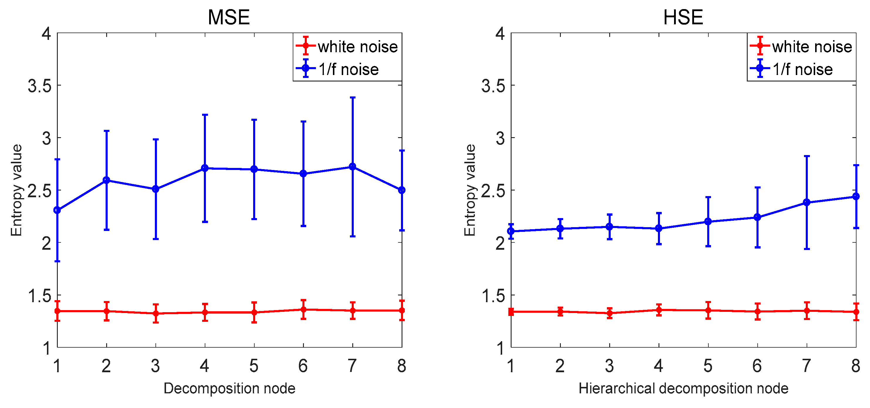
3.3. Comparison with Other Methods
4. Engineering Test Verification
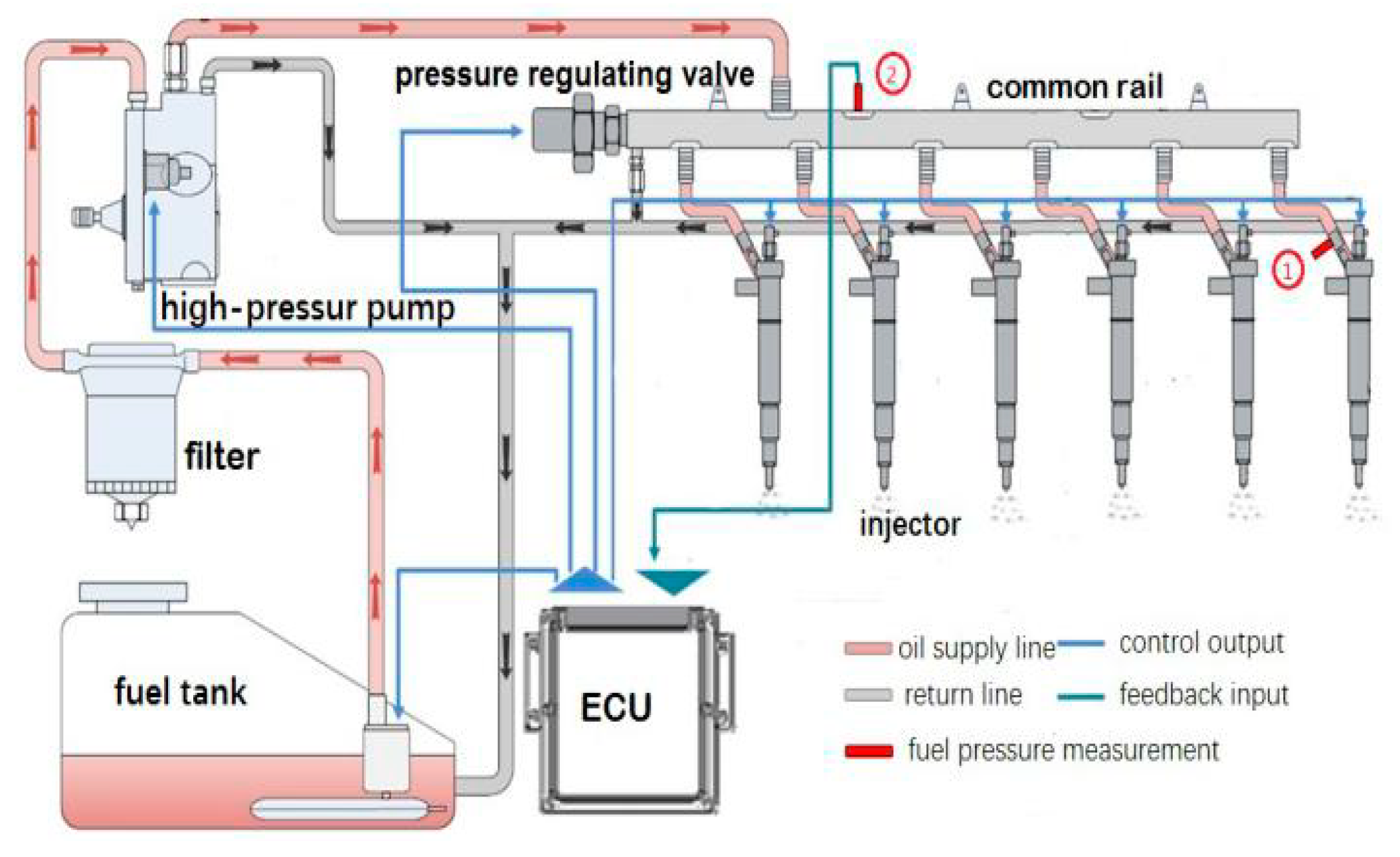
4.1. Signal Acquisition
4.2. Analysis of Test Data
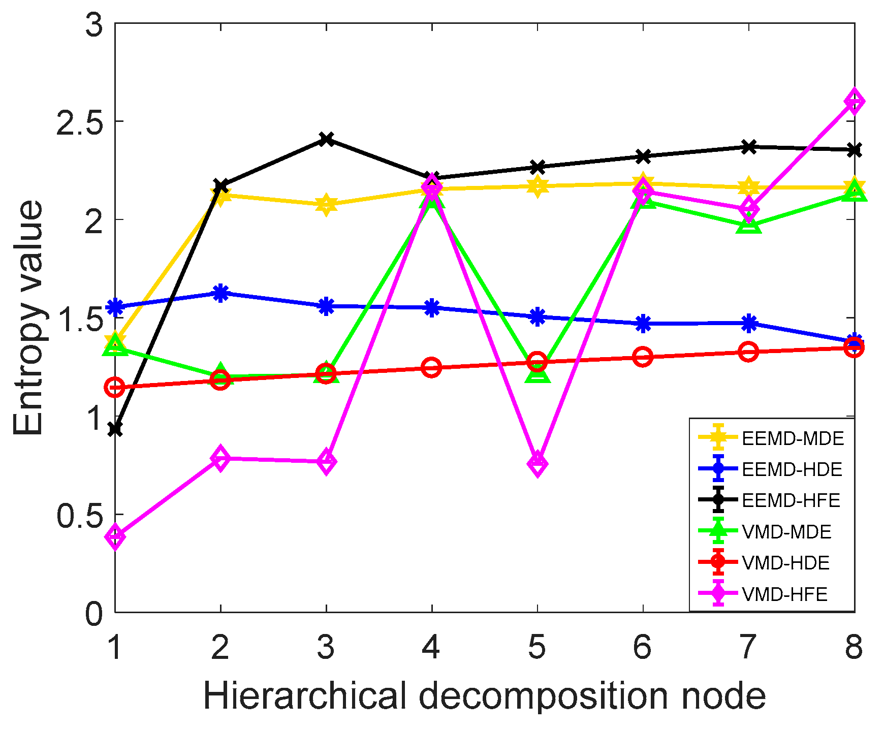
4.3. Comparative Study of Diagnostic Methods
5. Conclusions
Author Contributions
Funding
Acknowledgments
Conflicts of Interest
References
- Yang, Y.-S.; Ming, A.-B.; Zhang, Y.-Y.; Zhu, Y.-S. Discriminative non-negative matrix factorization (DNMF) and its application to the fault diagnosis of diesel engine. Mech. Syst. Sig. Process. 2017, 95, 158–171. [Google Scholar] [CrossRef]
- Kowalski, J.; Krawczyk, B.; Woźniak, M. Fault diagnosis of marine 4-stroke diesel engines using a one-vs-one extreme learning ensemble. Eng. Appl. Artif. Intell. 2017, 57, 134–141. [Google Scholar] [CrossRef]
- Gao, Z.; Ma, C.; Song, D.; Liu, Y. Deep quantum inspired neural network with application to aircraft fuel system fault diagnosis. Neurocomputing 2017, 238, 13–23. [Google Scholar] [CrossRef]
- Taghizadeh-Alisaraei, A.; Mahdavian, A. Fault detection of injectors in diesel engines using vibration time-frequency analysis. Appl. Acoust. 2019, 143, 48–58. [Google Scholar] [CrossRef]
- Lee, Y.; Lee, C.H. An uncertainty analysis of the time-resolved fuel injection pressure wave based on BOSCH method for a common rail diesel injector with a varying current wave pattern. J. Mech. Sci. Technol. 2018, 32, 5937–5945. [Google Scholar] [CrossRef]
- Yang, Y.; Peng, Z.; Zhang, W.; Meng, G. Parameterised time-frequency analysis methods and their engineering applications: A review of recent advances. Mech. Syst. Sig. Process. 2019, 119, 182–221. [Google Scholar] [CrossRef]
- Li, L.; Cai, H.; Jiang, Q.; Ji, H. An empirical signal separation algorithm for multicomponent signals based on linear time-frequency analysis. Mech. Syst. Sig. Process. 2019, 121, 791–809. [Google Scholar] [CrossRef]
- Sun, R.; Yang, Z.; Chen, X.; Tian, S.; Xie, Y. Gear fault diagnosis based on the structured sparsity time-frequency analysis. Mech. Syst. Sig. Process. 2018, 102, 346–363. [Google Scholar] [CrossRef]
- Wu, Y.; Li, X.; Wang, Y. Extraction and classification of acoustic scattering from underwater target based on Wigner-Ville distribution. Appl. Acoust. 2018, 138, 52–59. [Google Scholar] [CrossRef]
- Qu, H.; Li, T.; Chen, G. Synchro-squeezed adaptive wavelet transform with optimum parameters for arbitrary time series. Mech. Syst. Sig. Process. 2019, 114, 366–377. [Google Scholar] [CrossRef]
- Mohanty, S.; Gupta, K.K.; Raju, K.S. Hurst based vibro-acoustic feature extraction of bearing using EMD and VMD. Measurement 2018, 117, 200–220. [Google Scholar] [CrossRef]
- Lin, L.; Wang, Y.; Zhou, H. Iterative filtering as an alternative algorithm for empirical mode decomposition. Adv. Adapt. Data Anal. 2009, 1, 543–560. [Google Scholar] [CrossRef]
- Cicone, A.; Liu, J.; Zhou, H. Adaptive local iterative filtering for signal decomposition and instantaneous frequency analysis. Appl. Comput. Harmon. Anal. 2016, 41, 384–411. [Google Scholar] [CrossRef]
- Cicone, A. Nonstationary signal decomposition for dummies. In Advances in Mathematical Methods and High Performance Computing; Springer: Berlin, Germany, 2019; pp. 69–82. [Google Scholar]
- Cicone, A.; Zhou, H. Numerical Analysis for Iterative Filtering with New Efficient Implementations Based on FFT. arXiv Preprint 2018, arXiv:1802.01359. [Google Scholar]
- Wang, L.; Liu, Z.; Miao, Q.; Zhang, X. Time–frequency analysis based on ensemble local mean decomposition and fast kurtogram for rotating machinery fault diagnosis. Mech. Syst. Sig. Process. 2018, 103, 60–75. [Google Scholar] [CrossRef]
- Dragomiretskiy, K.; Zosso, D. Variational mode decomposition. IEEE Trans. Signal Process. 2013, 62, 531–544. [Google Scholar] [CrossRef]
- Bi, F.; Li, X.; Liu, C.; Tian, C.; Ma, T.; Yang, X. Knock detection based on the optimized variational mode decomposition. Measurement 2019, 140, 1–13. [Google Scholar] [CrossRef]
- Chen, X.; Yang, Y.; Cui, Z.; Shen, J. Vibration fault diagnosis of wind turbines based on variational mode decomposition and energy entropy. Energy 2019, 174, 1100–1109. [Google Scholar] [CrossRef]
- Li, G.; Tang, G.; Luo, G.; Wang, H. Underdetermined blind separation of bearing faults in hyperplane space with variational mode decomposition. Mech. Syst. Sig. Process. 2019, 120, 83–97. [Google Scholar] [CrossRef]
- Wu, L.; Yang, Y.; Maheshwari, M.; Li, N. Parameter optimization for FPSO design using an improved FOA and IFOA-BP neural network. Ocean Eng. 2019, 175, 50–61. [Google Scholar] [CrossRef]
- Wang, L.; Lv, S.-X.; Zeng, Y.-R. Effective sparse adaboost method with ESN and FOA for industrial electricity consumption forecasting in China. Energy 2018, 155, 1013–1031. [Google Scholar] [CrossRef]
- Cheng, J.; Xiong, Y. The quality evaluation of classroom teaching based on FOA-GRNN. Procedia Comput. Sci. 2017, 107, 355–360. [Google Scholar] [CrossRef]
- Han, S.-Z.; Huang, L.-H.; Zhou, Y.-Y.; Liu, Z.-L. Mixed chaotic FOA with GRNN to construction of a mutual fund forecasting model. Cognit. Syst. Res. 2018, 52, 380–386. [Google Scholar] [CrossRef]
- Pincus, S. Approximate entropy (ApEn) as a complexity measure. Chaos: An Interdisciplinary Journal of Nonlinear Science 1995, 5, 110–117. [Google Scholar] [CrossRef] [PubMed]
- Richman, J.S.; Moorman, J.R. Physiological time-series analysis using approximate entropy and sample entropy. Am. J. Physiol. Heart Circ. Physiol. 2000, 278, H2039–H2049. [Google Scholar] [CrossRef] [PubMed]
- Costa, M.; Goldberger, A.L.; Peng, C.-K. Multiscale entropy analysis of biological signals. Phys. Rev. E 2005, 71, 021906. [Google Scholar] [CrossRef] [PubMed]
- Costa, M.; Goldberger, A.L.; Peng, C.-K. Multiscale entropy analysis of complex physiologic time series. Phys. Rev. Lett. 2002, 89, 068102. [Google Scholar] [CrossRef] [PubMed]
- Zheng, J.; Pan, H.; Cheng, J. Rolling bearing fault detection and diagnosis based on composite multiscale fuzzy entropy and ensemble support vector machines. Mech. Syst. Sig. Process. 2017, 85, 746–759. [Google Scholar] [CrossRef]
- Jiang, Y.; Peng, C.-K.; Xu, Y. Hierarchical entropy analysis for biological signals. J. Comput. Appl. Math. 2011, 236, 728–742. [Google Scholar] [CrossRef]
- Rostaghi, M.; Azami, H. Dispersion entropy: A measure for time-series analysis. IEEE Signal Process Lett. 2016, 23, 610–614. [Google Scholar] [CrossRef]
- Azami, H.; Arnold, S.E.; Sanei, S.; Chang, Z.; Sapiro, G.; Escudero, J.; Gupta, A.S. Multiscale Fluctuation-based Dispersion Entropy and its Applications to Neurological Diseases. IEEE Access 2019, 7, 68718–68733. [Google Scholar] [CrossRef]
- Yao, P.; Zhou, K.; Zhu, Q. Quantitative evaluation method of arc sound spectrum based on sample entropy. Mech. Syst. Sig. Process. 2017, 92, 379–390. [Google Scholar] [CrossRef]
- Si, L.; Wang, Z.; Liu, X.; Tan, C. A sensing identification method for shearer cutting state based on modified multi-scale fuzzy entropy and support vector machine. Eng. Appl. Artif. Intell. 2019, 78, 86–101. [Google Scholar] [CrossRef]
- Zheng, J.; Dong, Z.; Pan, H.; Ni, Q.; Liu, T.; Zhang, J. Composite multi-scale weighted permutation entropy and extreme learning machine based intelligent fault diagnosis for rolling bearing. Measurement 2019, 143, 69–80. [Google Scholar] [CrossRef]
- Zhu, K.; Song, X.; Xue, D. A roller bearing fault diagnosis method based on hierarchical entropy and support vector machine with particle swarm optimization algorithm. Measurement 2014, 47, 669–675. [Google Scholar] [CrossRef]
- Naik, J.; Dash, P.K.; Dhar, S. A multi-objective wind speed and wind power prediction interval forecasting using variational modes decomposition based Multi-kernel robust ridge regression. Renew. Energy 2019, 136, 701–731. [Google Scholar] [CrossRef]
- Lian, J.; Liu, Z.; Wang, H.; Dong, X. Adaptive variational mode decomposition method for signal processing based on mode characteristic. Mech. Syst. Sig. Process. 2018, 107, 53–77. [Google Scholar] [CrossRef]
- Liu, J.; Li, Y.-F.; Zio, E. A SVM framework for fault detection of the braking system in a high speed train. Mech. Syst. Sig. Process. 2017, 87, 401–409. [Google Scholar] [CrossRef]


| Signal Length N | 128 | 512 | 1024 | 4096 |
|---|---|---|---|---|
| White noise | 0.0446 | 0.0237 | 0.0105 | 0.0022 |
| 1/f noise | 0.0527 | 0.021 | 0.0114 | 0.0026 |
| Embedding Dimension m | 2 | 3 | 4 | 5 |
|---|---|---|---|---|
| White noise | 0.0028 | 0.0118 | 0.0065 | 0.0026 |
| 1/f noise | 0.0022 | 0.0055 | 0.0052 | 0.0023 |
| Class c | 3 | 4 | 5 | 6 | 7 | 8 | 9 | 10 |
|---|---|---|---|---|---|---|---|---|
| White noise | 0.0053 | 0.0082 | 0.0105 | 0.0115 | 0.0115 | 0.0168 | 0.0128 | 0.0123 |
| 1/f noise | 0.0014 | 0.0022 | 0.0024 | 0.0024 | 0.0021 | 0.0029 | 0.0029 | 0.0043 |
| Information Entropy Method | MSE | HSE | MFE | HFE | MDE | HDE |
|---|---|---|---|---|---|---|
| White noise | 0.0601 | 0.0385 | 0.0406 | 0.0338 | 0.0291 | 0.0061 |
| 1/f noise | 0.1885 | 0.0696 | 0.0455 | 0.0354 | 0.0233 | 0.0062 |
| Method | EEMD-HFE | EEMD-MDE | EEMD-HDE | VMD-HFE | VMD-MDE | VMD-HDE |
|---|---|---|---|---|---|---|
| CV/10−16 | 4.72 | 3.87 | 2.57 | 4.52 | 2.88 | 2.03 |
| Time/s | 17.858 | 2.932 | 1.985 | 16.985 | 2.287 | 1.941 |
| Method | EEMD-HFE | EEMD-MDE | EEMD-HDE | VMD-HFE | VMD-MDE | VMD-HDE |
|---|---|---|---|---|---|---|
| Classification accuracy/% | 88.8 | 92.2 | 93.3 | 95.5 | 97.7 | 100 |
| Time/s | 20.8 | 11.9 | 11.4 | 13.7 | 4.7 | 4.2 |
© 2019 by the authors. Licensee MDPI, Basel, Switzerland. This article is an open access article distributed under the terms and conditions of the Creative Commons Attribution (CC BY) license (http://creativecommons.org/licenses/by/4.0/).
Share and Cite
Song, E.; Ke, Y.; Yao, C.; Dong, Q.; Yang, L. Fault Diagnosis Method for High-Pressure Common Rail Injector Based on IFOA-VMD and Hierarchical Dispersion Entropy. Entropy 2019, 21, 923. https://doi.org/10.3390/e21100923
Song E, Ke Y, Yao C, Dong Q, Yang L. Fault Diagnosis Method for High-Pressure Common Rail Injector Based on IFOA-VMD and Hierarchical Dispersion Entropy. Entropy. 2019; 21(10):923. https://doi.org/10.3390/e21100923
Chicago/Turabian StyleSong, Enzhe, Yun Ke, Chong Yao, Quan Dong, and Liping Yang. 2019. "Fault Diagnosis Method for High-Pressure Common Rail Injector Based on IFOA-VMD and Hierarchical Dispersion Entropy" Entropy 21, no. 10: 923. https://doi.org/10.3390/e21100923
APA StyleSong, E., Ke, Y., Yao, C., Dong, Q., & Yang, L. (2019). Fault Diagnosis Method for High-Pressure Common Rail Injector Based on IFOA-VMD and Hierarchical Dispersion Entropy. Entropy, 21(10), 923. https://doi.org/10.3390/e21100923