Precipitation Complexity and its Spatial Difference in the Taihu Lake Basin, China


Abstract
1. Introduction
2. Data and Methods
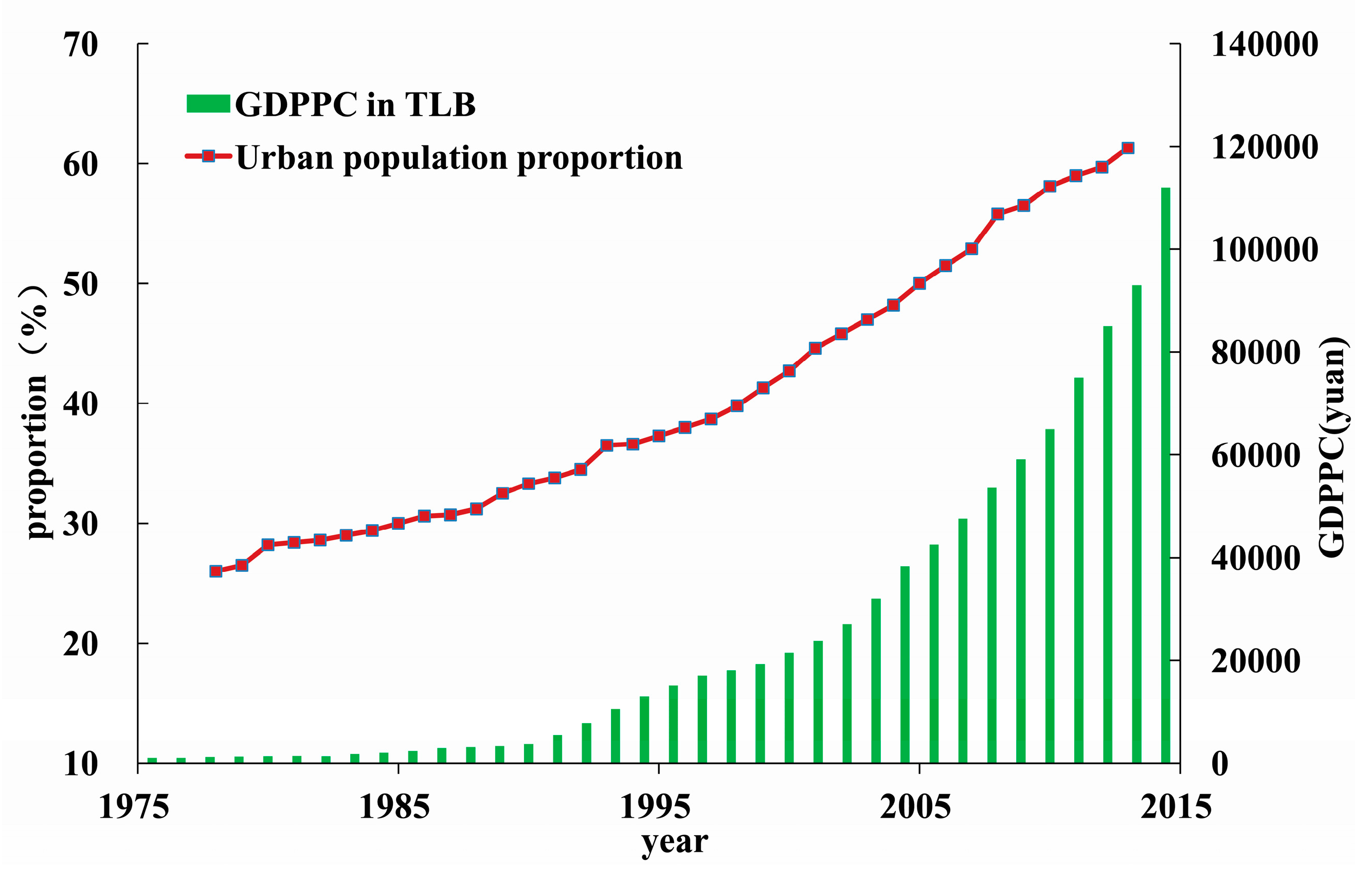
2.1. Study Area
2.2. Data Used
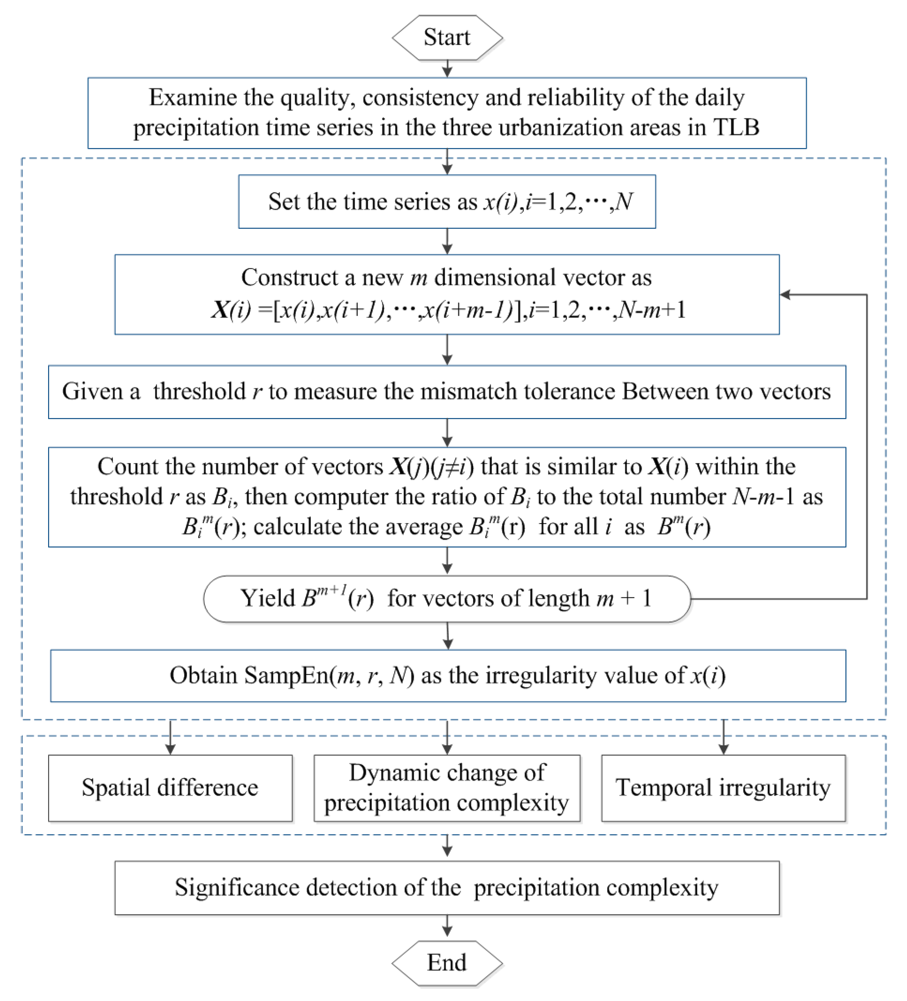
2.3. Methods
3. Results and Discussion
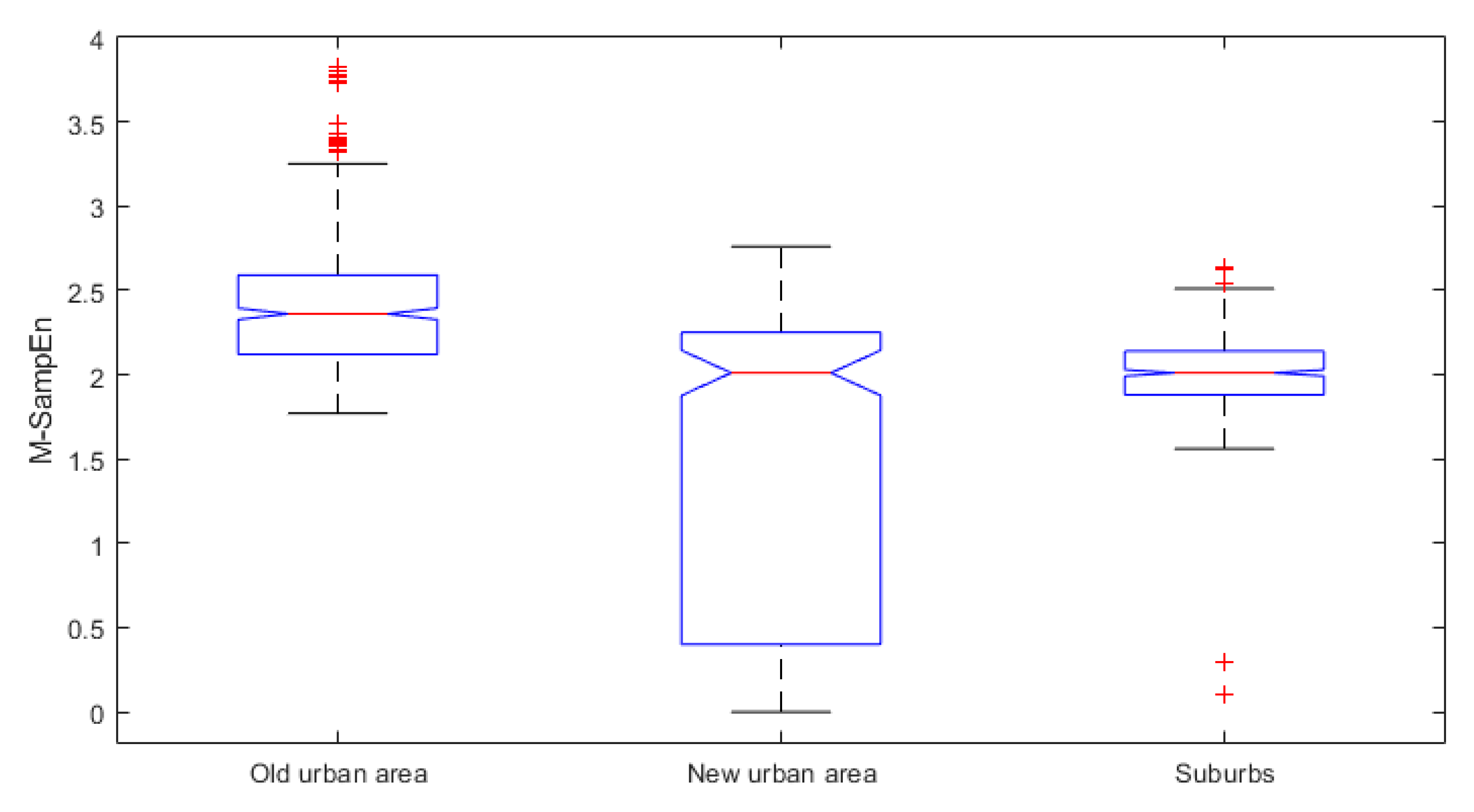
3.1. Spatial Difference of Precipitation Complexity in TLB
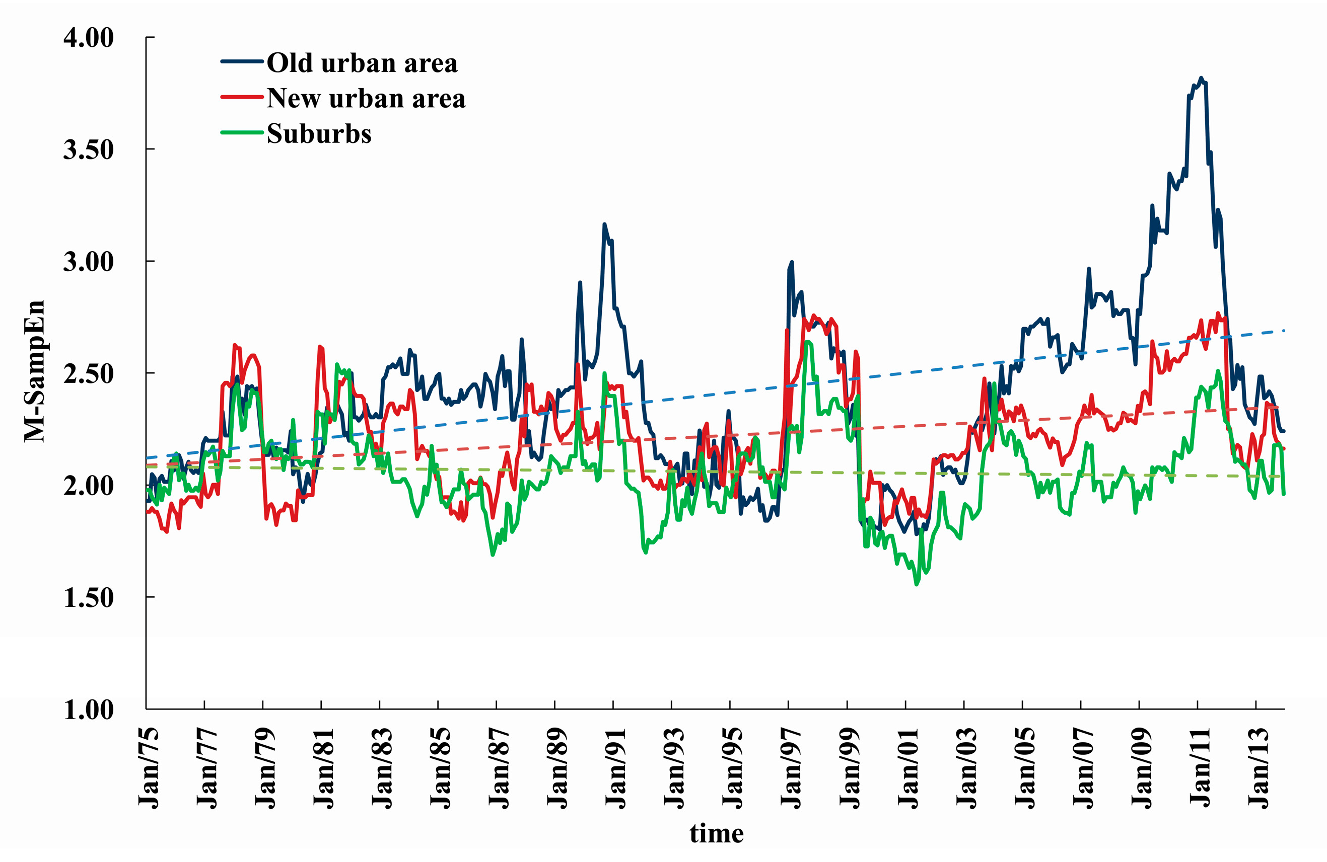
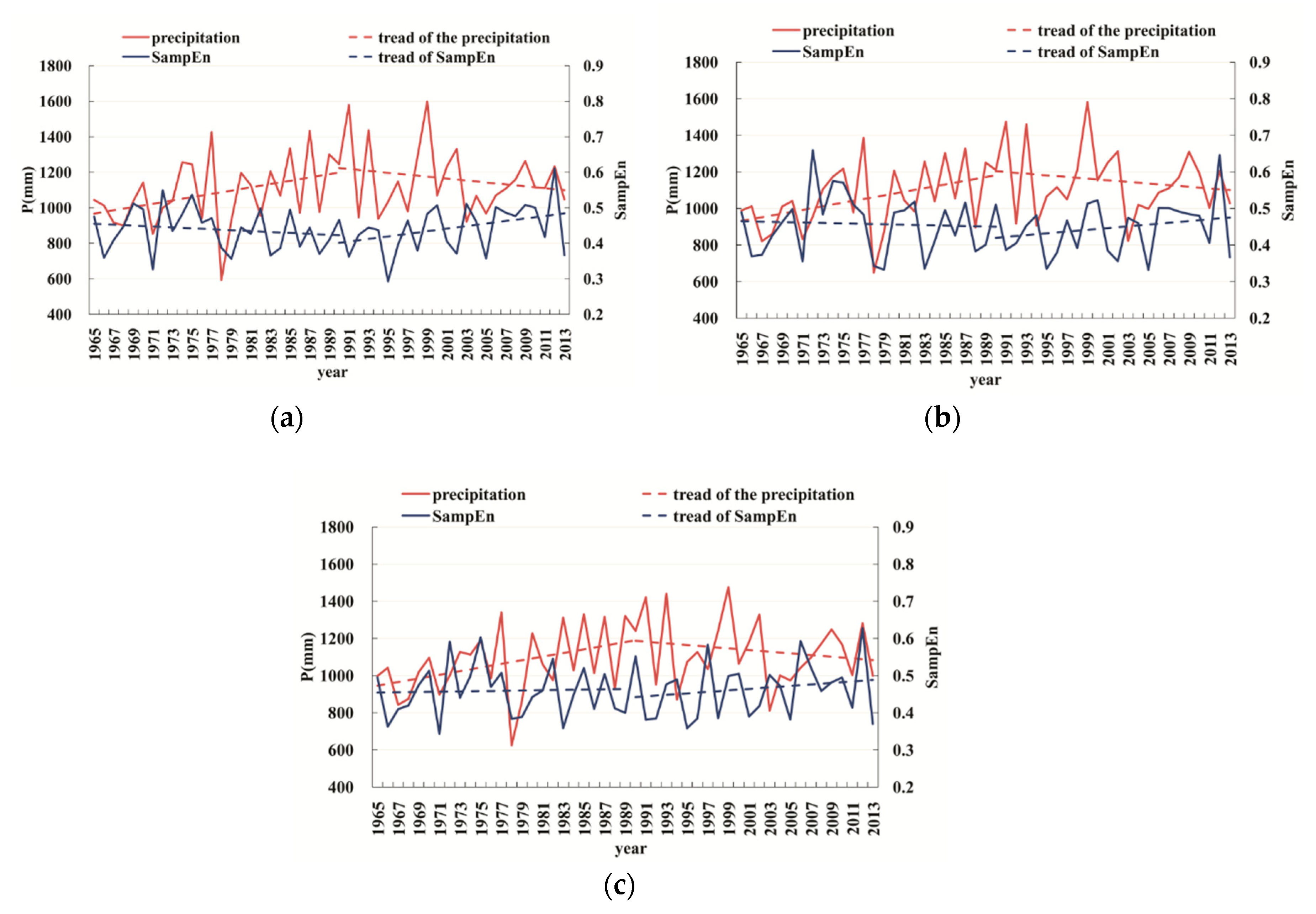
3.2. Dynamic Change of Precipitation Complexity in TLB
3.3. Temporal Complexity of Precipitation in TLB
4. Conclusions
Author Contributions
Funding
Acknowledgments
Conflicts of Interest
References
- Haddeland, I.; Heinke, J.; Biemans, H.; Eisner, S.; Flörke, M.; Hanasaki, N.; Konzmann, M.; Ludwig, F.; Masaki, Y.; Schewe, J.; et al. Global water resources affected by human interventions and climate change. Proc. Natl. Acad. Sci. USA 2014, 111, 3251–3256. [Google Scholar] [CrossRef] [PubMed]
- Grill, G.; Lehner, B.; Lumsdon, A.E.; MacDonald, G.K.; Zarfl, C.; Liermann, C.R. An index-based framework for assessing patterns and trends in river fragmentation and flow regulation by global dams at multiple scales. Environ. Res. Lett. 2015, 10, 015001. [Google Scholar] [CrossRef]
- Xue, L.Q.; Liu, Y.H.; Zhang, M.Z.; Wang, S.Q.; Li, J. Mutation Test on Rainfall and Runoff Time Series Based on Sample Entropy. J. Earth Sci. Environ. 2015, 37, 75–80. [Google Scholar]
- Hu, Q.F.; Zhang, J.Y.; Wang, Y.T.; Huang, Y.; Liu, Y.; Li, L.J. A review of urbanization impact on precipitation. Adv. Water Sci. 2018, 29, 138–150. [Google Scholar]
- Ravines, R.R.; Schmidt, A.M.; Migon, H.S.; Renno, C.D. A joint model for rainfall-runoff: The case of Rio Grande Basin. J. Hydrol. 2008, 353, 189–200. [Google Scholar] [CrossRef]
- Sang, Y.F.; Wang, D.; Wu, J.C.; Zhu, Q.P.; Wang, L. The relation between periods’ identification and noises in hydrologic series data. J. Hydrol. 2009, 368, 165–177. [Google Scholar] [CrossRef]
- Sang, Y.F.; Singh, V.P.; Hu, Z.; Xie, P.; Li, X. Entropy-aided evaluation of meteorological droughts over China. J. Geophys. Res. Atmos. 2018, 123. [Google Scholar] [CrossRef]
- Shahin, M.; Oorschot, H.J.L.V.; Lange, S.J.D. Statistical analysis in water resources engineering. Opt. Express 1993, 22, 7362–7363. [Google Scholar]
- Machiwal, D.; Jha, M.K. Hydrologic Time Series Analysis: Theory and Practice; Springer: Amsterdam, The Netherlands, 2012. [Google Scholar]
- Sang, Y.F.; Sun, F.; Singh, V.P.; Xie, P.; Sun, J. A discrete wavelet spectrum approach for identifying non-monotonic trends in hydroclimate data. Hydrol. Earth Syst. Sci. 2018, 22, 757–766. [Google Scholar] [CrossRef]
- Xie, P.; Wu, Z.; Sang, Y.F.; Gu, H.; Zhao, Y.; Singh, V.P. Evaluation of the significance of abrupt changes in precipitation and runoff process in China. J. Hydrol. 2018, 560, 451–460. [Google Scholar] [CrossRef]
- Kite, G. Use of time series analysis to detect climatic change. J. Hydrol. 1989, 111, 259–279. [Google Scholar] [CrossRef]
- Tetzlaff, D.; Carey, S.K.; McNamara, J.P.; Laudon, H.; Soulsby, C. The essential value of long-term experimental data for hydrology and water management. Water Resour. Res. 2017, 53, 2598–2604. [Google Scholar] [CrossRef]
- Sang, Y.F.; Singh, V.P.; Wen, J.; Liu, C.M. Gradation of complexity and predictability of hydrological processes. J. Geophys. Res.-Atmos. 2015, 120, 5334–5343. [Google Scholar] [CrossRef]
- Shannon, C.E. A Mathematical Theory of Communication. Bell Syst. Tech. J. 1948, 27, 379–423. [Google Scholar] [CrossRef]
- Singh, V.P. Entropy theory for hydrologic modeling. J. Beijing Norm. Univ. Nat. Sci. 2010, 46, 229–240. [Google Scholar]
- Chen, L.; Singh, V.P. Entropy-based derivation of generalized distributions for hydrometeorological frequency analysis. J. Hydrol. 2018, 557, 699–712. [Google Scholar] [CrossRef]
- Singh, V.P.; Sivakumar, B.; Cui, H.J. Tsallis Entropy Theory for Modeling in Water Engineering: A Review. Entropy 2017, 19, 641. [Google Scholar] [CrossRef]
- Singh, V.P.; Oh, J. A Tsallis entropy-based redundancy measure for water distribution network. Phys. A 2014, 421, 360–376. [Google Scholar] [CrossRef]
- Papalexiou, S.M.; Koutsoyiannis, D. Entropy based derivation of probability distributions: A case study to daily rainfall. Adv. Water Resour. 2012, 45, 51–57. [Google Scholar] [CrossRef]
- Krstanovic, P.F.; Singh, V.P. Evaluation of rainfall networks using entropy: 1. Theoretical development. Water Resour. Manag. 1992, 6, 279–293. [Google Scholar] [CrossRef]
- Krstanovic, P.F.; Singh, V.P. Evaluation of rainfall networks using entropy: 2. Application. Water Resour. Manag. 1992, 6, 295–314. [Google Scholar] [CrossRef]
- Pincus, S.M. Approximate entropy as a measure of system complexity. Proc. Natl. Acad. Sci. USA 1991, 88, 2297–2301. [Google Scholar] [CrossRef] [PubMed]
- Pincus, S.M. Approximate entropy (ApEn) as a complexity measure. Chaos 1995, 5, 110–117. [Google Scholar] [CrossRef] [PubMed]
- Li, X.G.; Wei, N.; Wei, X. A new method for determining parameters of system complexity measures and its application. Syst. Eng.-Theory Pract. 2018, 38, 252–262. [Google Scholar]
- Richman, J.S.; Moorman, J.R. Physiological time-series analysis using approximate entropy and sample entropy. Am. J. Physiol. Heart Circ. Physiol. 2000, 278, 2039–2049. [Google Scholar] [CrossRef] [PubMed]
- Manis, G. Fast computation of approximate entropy. Comput. Methods Prog. Biomed. 2008, 91, 48–54. [Google Scholar] [CrossRef] [PubMed]
- Lake, D.E.; Richman, J.S.; Griffin, M.P.; Moorman, J.R. Sample entropy analysis of neonatal heart rate variability. Am. J. Physiol. 2002, 283, 789–797. [Google Scholar] [CrossRef] [PubMed]
- Pincus, S.M. Assessing serial irregularity and its implications for health. Ann. N. Y. Acad. Sci. 2002, 954, 245–267. [Google Scholar] [CrossRef]
- Zhao, Z.H.; Yang, S.P. Sample entropy-based roller bearing fault diagnosis method. J. Vib. Shock 2012, 31, 136–140. [Google Scholar]
- Hu, X.S.; Jiang, J.C.; Cao, D.P.; Egardt, B. Battery Health Prognosis for Electric Vehicles Using Sample Entropy and Sparse Bayesian Predictive Modeling. IEEE Trans. Ind. Electron. 2016, 63, 2645–2656. [Google Scholar] [CrossRef]
- Peng, T.; Chen, X.H.; Zhuang, C.B. Analysis on complexity of monthly runoff series based on sample entropy in the Dongjiang river. Ecol. Environ. Sci. 2009, 18, 1379–1382. [Google Scholar]
- Kang, Y.; Cai, H.J.; Song, S.B. Study and application of complexity model for hydrological system. J. Hydroelectr. Eng. 2013, 32, 5–10. [Google Scholar]
- Chou, C.M. Complexity analysis of rainfall and runoff time series based on sample entropy in different temporal scales. Stoch. Environ. Res. Risk Assess 2014, 28, 1401–1408. [Google Scholar] [CrossRef]
- Wu, H.Y.; Wang, Y.T.; Hu, Q.F.; Liu, Y. Tempo-spatial Change of Precipitation in Taihu Lake Basin during Recent 61 Years. J. China Hydrol. 2013, 33, 75–81. [Google Scholar]
- Wu, J.; Lin, H.J.; Wu, Z.Y.; Jiang, G.H.; Ji, T.D. Influence of El Nino Events on Rainfall in Taihu Basin. J. China Hydrol. 2017, 37, 60–65. [Google Scholar] [CrossRef]
- Ji, D.; Zhang, H.; Shen, W.S.; Wang, Q.; Li, H.D.; Lin, N.F. The Response Relationship between Underlying Surface Changing and Climate Change in the Taihu Basin. J. Nat. Resour. 2013, 28, 51–62. [Google Scholar]
- Ding, J.J.; Xu, Y.P.; Pan, G.B. Effect of urbanization on regional precipitation in Suzhou-Wuxi-Changzhou area. Resour. Environ. Yangtze Basin 2010, 19, 873–877. [Google Scholar]
- Yang, M.N.; Xu, Y.P.; Pan, G.B.; Han, L.F. Impacts of urbanization on precipitation in Taihu Lake Basin, China. J. Hydrol. Eng. 2014, 19, 739–746. [Google Scholar] [CrossRef]
- Jin, Y.R.; Hu, Q.F.; Wang, Y.T.; Huang, Y.; Yang, H.B.; Cui, T.T. Impacts of rapid urbanization on precipitation at two representative rain gauges in Shanghai City. J. Hohai Univ. (Nat. Sci.) 2017, 45, 1–8. [Google Scholar]
- Lin, H.; Sun, J.N. Possible effects of urbanization on regional precipitation over Yangtze River Delta area. J. Nanjing Univ. (Natl. Sci.) 2014, 50, 792–799. [Google Scholar]
- Li, N.; Xu, Y.P.; Chen, S. Influence of Urbanization on Precipitation in Suzhou City. Resour. Environ. Yangtze Basin 2006, 15, 335–339. [Google Scholar]


| Urbanization Zone | Old Urban Area | New Urban Area | Suburbs |
|---|---|---|---|
| * (mm) | 1118.1 | 1100.1 | 1097.5 |
| SampEn value | 2.168 | 2.103 | 2.066 |
| Source | Variance Sum | Degree of Freedom | Mean Value of Variance | Statistic Value F | Prob > F |
|---|---|---|---|---|---|
| Columns | 154.822 | 2 | 77.411 | 171.61 | 2.170 × 10−67 |
| Error | 631.953 | 1401 | 0.451 | ||
| Total | 786.775 | 1403 |
| Urbanization Zone | Trend | |||
|---|---|---|---|---|
| Old urban area | Before 1990 | 1.94 | 1.64 | significant upward |
| After 1990 | −0.12 | 1.64 | insignificant | |
| New urban area | Before 1990 | 2.42 | 1.64 | significant upward |
| After 1990 | −0.42 | 1.64 | insignificant | |
| Suburbs | Before 1990 | 2.07 | 1.64 | significant upward |
| After 1990 | −0.47 | 1.64 | insignificant | |
| Urbanization Zone | Old Urban Area | New Urban Area | Suburbs | |
|---|---|---|---|---|
| * (mm) | Before 1990 | 1082.75 | 1056.55 | 1067.99 |
| After 1990 | 1158.05 | 1149.36 | 1130.75 | |
| Before 1990 | 9.2494 | 9.9483 | 9.7686 | |
| After 1990 | −5.4297 | −4.4789 | −4.4862 | |
| Before 1990 | −0.0013 | −0.0006 | 0.0004 | |
| After 1990 | 0.0036 | 0.0024 | 0.002 | |
| u | 0.00033 | 0.00021 | 0.00011 | |
© 2019 by the authors. Licensee MDPI, Basel, Switzerland. This article is an open access article distributed under the terms and conditions of the Creative Commons Attribution (CC BY) license (http://creativecommons.org/licenses/by/4.0/).
Share and Cite
Hu, J.; Liu, Y.; Sang, Y.-F. Precipitation Complexity and its Spatial Difference in the Taihu Lake Basin, China. Entropy 2019, 21, 48. https://doi.org/10.3390/e21010048
Hu J, Liu Y, Sang Y-F. Precipitation Complexity and its Spatial Difference in the Taihu Lake Basin, China. Entropy. 2019; 21(1):48. https://doi.org/10.3390/e21010048
Chicago/Turabian StyleHu, Jian, Yong Liu, and Yan-Fang Sang. 2019. "Precipitation Complexity and its Spatial Difference in the Taihu Lake Basin, China" Entropy 21, no. 1: 48. https://doi.org/10.3390/e21010048
APA StyleHu, J., Liu, Y., & Sang, Y.-F. (2019). Precipitation Complexity and its Spatial Difference in the Taihu Lake Basin, China. Entropy, 21(1), 48. https://doi.org/10.3390/e21010048