Approximate Bayesian Computation for Estimating Parameters of Data-Consistent Forbush Decrease Model


Abstract
1. Introduction
2. Applied Methodology
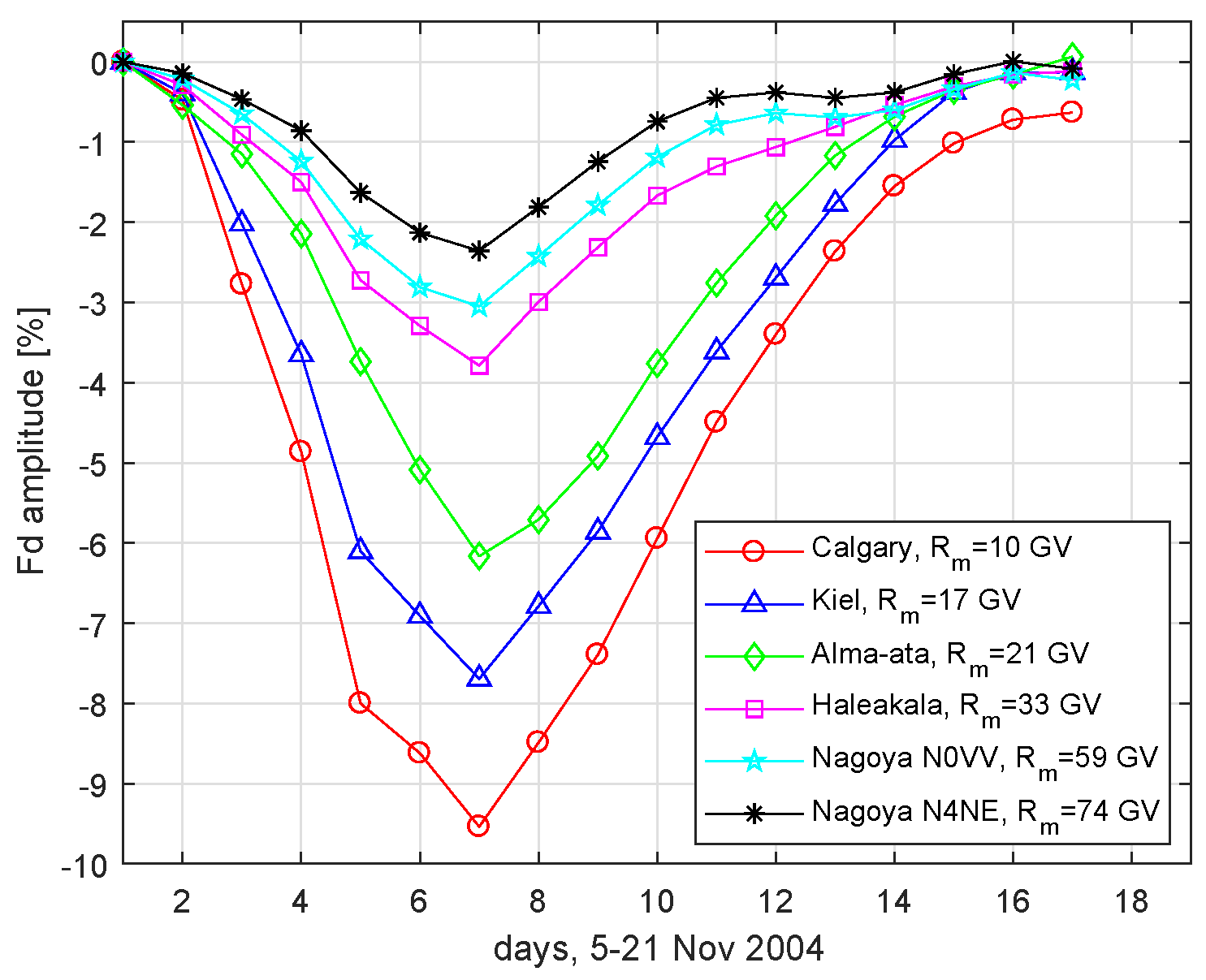
2.1. Stochastic Model of the Forbush Decrease of GCR Intensity
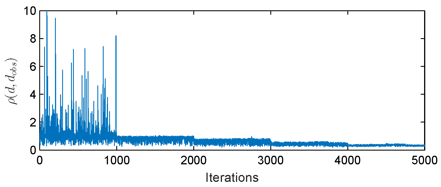
2.2. Approximate Bayesian Computation Algorithm
| Algorithm 1 ABC SMC |
|
2.2.1. Threshold Schedule Updating Scheme
- The distribution of measure of samples set is discrete, thus some approximation is required. To keep the procedure flexible and support the interval the best choice for continuous distributions seems to be the family of distributions.
- We propose to define the value of to be dependent on the ratio between a number of currently accepted samples (AS) and the number of all hitherto generated samples (AGS) i.e., .
2.2.2. Transition Kernel
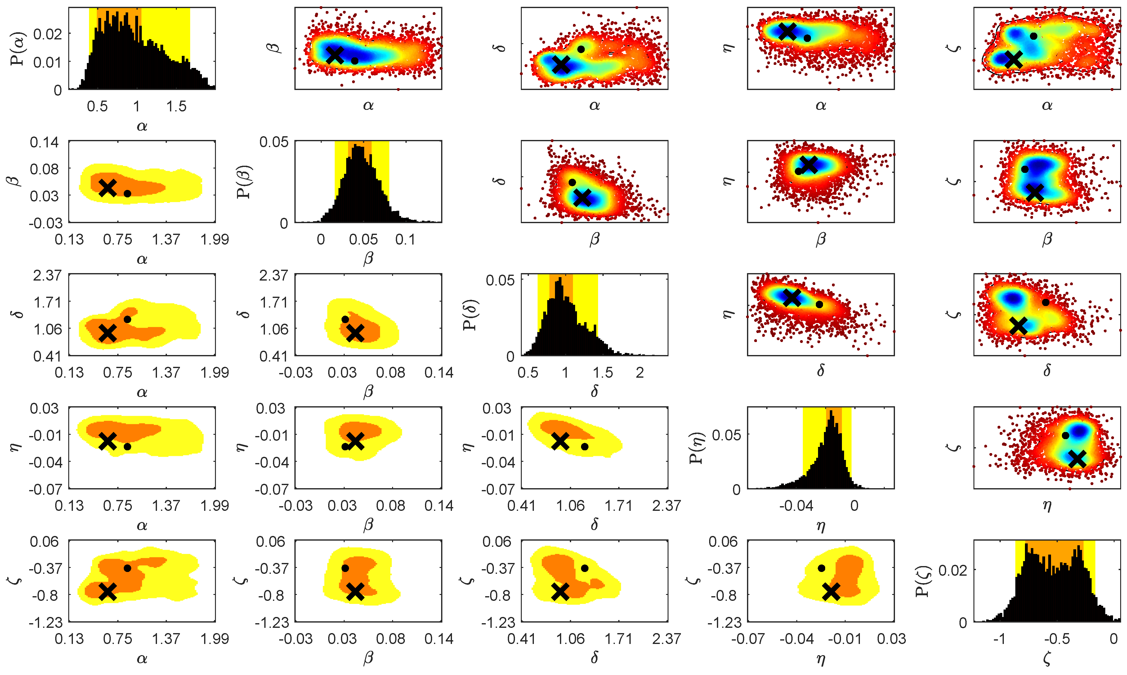
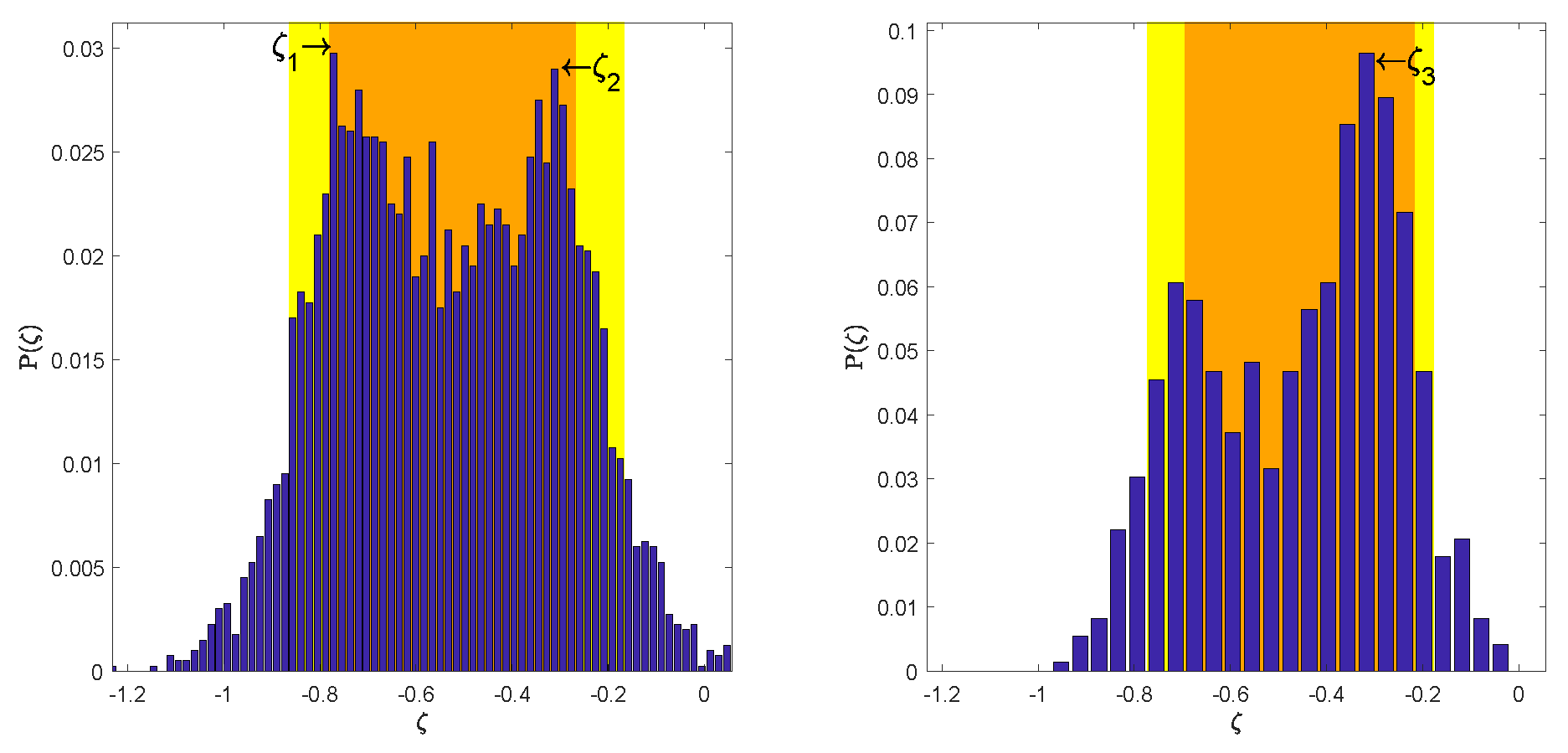
3. Results
4. Summary
Author Contributions
Funding
Acknowledgments
Conflicts of Interest
Abbreviations
| ABC | Approximate Bayesian Computation |
| ABC SMC | Approximate Bayesian Computation with Sequential Monte Carlo |
| AGS | All hitherto Generated Samples |
| AS | All Samples |
| FB | Fractional Bias |
| Fd | Forbush decrease |
| GCR | Galactic Cosmic Rays |
| IMF | Interplanetary Magnetic Field |
| PSD | Power Spectral Density |
| SMC | Sequential Monte Carlo |
| SDE | Stochastic Differential Equation |
References
- Mavromichalaki, H.; Papaioannou, A.; Plainaki, C.; Sarlanis, C.; Souvatzoglou, G.; Gerontidou, M.; Papailiou, M.; Eroshenko, E.; Belov, A.; Yanke, V.; et al. Applications and usage of the real-time Neutron Monitor Database. Adv. Space Res. 2011, 47, 2210–2222. [Google Scholar] [CrossRef]
- Forbush, S.E. World-wide cosmic ray variations 1937–1952. Geophys. Res. 1954, 59, 525–542. [Google Scholar] [CrossRef]
- Simpson, J.A. Cosmic-Radiation Intensity-Time Variations and Their Origin. III. The Origin of 27-Day Variations. Phys. Rev. 1954, 94, 426–440. [Google Scholar] [CrossRef]
- Zhang, G.; Burlaga, L.F. Magnetic clouds, geomagnetic disturbances, and cosmic ray decreases. J. Geophys. Res. 1988, 93, 2511–2518. [Google Scholar] [CrossRef]
- Lockwood, J.A.; Webber, W.R.; Jokipii, J.R. Characteristic recovery times of Forbush-type decreases in the cosmic radiation: 1. Observations at Earth at different energies. J. Geophys. Res. 1986, 91, 2851–2857. [Google Scholar] [CrossRef]
- Yu, X.X.; Lu, H.; Le, G.M.; Shi, F. Influence of Magnetic Clouds on Variations of Cosmic Rays in November 2004. Sol. Phys. 2010, 263, 223–237. [Google Scholar] [CrossRef]
- Arunbabu, K.P.; Antia, H.M.; Dugad, S.R.; Gupta, S.K.; Hayashi, Y.; Kawakami, S.; Mohanty, P.K.; Oshima, A.; Subramanian, P. How are Forbush decreases related to interplanetary magnetic field enhancements? Astron. Astrophys. 2015, 580, A41. [Google Scholar] [CrossRef]
- Wawrzynczak, A.; Alania, M.V. Modeling and data analysis of a Forbush decrease. Adv. Space Res. 2010, 45, 622–631. [Google Scholar] [CrossRef]
- Alania, M.V.; Wawrzynczak, A. Energy dependence of the rigidity spectrum of Forbush decrease of galactic cosmic ray intensity. Adv. Space Res. 2012, 50, 725–730. [Google Scholar] [CrossRef]
- Wawrzynczak, A.; Alania, M.V. The connection of the interplanetary magnetic field turbulence and rigidity spectrum of Forbush decrease of the galactic cosmic ray intensity. J. Phys. Conf. Ser. 2015, 632, 1742–6596. [Google Scholar] [CrossRef]
- Jokipii, J.R. Cosmic-Ray Propagation. I. Charged Particles in a Random Magnetic Field. Astrophys. J. 1966, 146, 480–487. [Google Scholar] [CrossRef]
- Shalchi, A. Nonlinear Cosmic Ray Diffusion Theories; Springer: Berlin, Germany, 2009. [Google Scholar]
- Green, P.J.; Łatuszynski, K.; Pereyra, M.; Robert, C.P. Bayesian computation: A summary of the current state, and samples backwards and forwards. Stat. Comput. 2015, 25, 835–862. [Google Scholar] [CrossRef]
- Sunnaker, M.; Busetto, A.G.; Numminen, E.; Corander, J.; Foll, M.; Dessimoz, C. Approximate Bayesian computation. PLoS Comput. Biol. 2013, 9, e1002803. [Google Scholar] [CrossRef] [PubMed]
- Parker, E. The passage of energetic charged particles through interplanetary space. Planet. Space Sci. 1965, 13, 9–49. [Google Scholar] [CrossRef]
- Wawrzynczak, A.; Modzelewska, R.; Gil, A. Stochastic approach to the numerical solution of the non-stationary Parker’s transport equation. J. Phys. Conf. Ser. 2015, 574, 012078. [Google Scholar] [CrossRef]
- Wawrzynczak, A.; Modzelewska, R.; Gil, A. Algorithms for Forward and Backward Solution of the Fokker-Planck Equation in the Heliospheric Transport of Cosmic Rays. LNCS 2018, 1077, 14–23. [Google Scholar] [CrossRef]
- Gardiner, C.W. Handbook of Stochastic Methods. For Physics, Chemistry and the Natural Sciences; Springer: Berlin, Germany; New York, NY, USA, 2004. [Google Scholar]
- Alania, M.V. Stochastic variations of galactic cosmic rays. Acta Phys. Pol. B 2002, 33, 1149–1166. [Google Scholar]
- Kopp, A.; Busching, I.; Strauss, R.D.; Potgieter, M.S. A stochastic differential equation code for multidimensional Fokker–Planck type problems. Comput. Phys. Commun. 2012, 183, 530–542. [Google Scholar] [CrossRef]
- Wawrzynczak, A.; Modzelewska, R.; Kluczek, M. Numerical methods for solution of the stochastic differential equations equivalent to the nonstationary Parkers transport equation. J. Phys. Conf. Ser. 2015, 633, 1742–6596. [Google Scholar] [CrossRef]
- Beaumont, M.A.; Zhang, W.; Balding, D.J. Approximate Bayesian computation in population genetics. Genetics 2002, 162, 2025–2035. [Google Scholar] [PubMed]
- Marin, J.M.; Pudlo, P.; Robert, C.P.; Ryder, R.J. Approximate bayesian computational methods. Stat. Comput. 2012, 22, 1167–1180. [Google Scholar] [CrossRef]
- Del Moral, P.; Doucet, A.; Jasra, A. An adaptive sequential Monte Carlo method for approximate Bayesian computation. Stat. Comput. 2012, 22, 1009–1020. [Google Scholar] [CrossRef]
- Silk, D.; Filippi, S.; Stumpf, M.P. Optimizing threshold-schedules for sequential approximate Bayesian computation: Applications to molecular systems. Stat. Appl. Genet. Mol. Biol. 2013, 12, 1–16. [Google Scholar] [CrossRef] [PubMed]
- Filippi, S.; Barnes, C.P.; Cornebise, J.; Stumpf, M.P. On optimality of kernels for approximate Bayesian computation using sequential Monte Carlo. Stat. Appl. Genet. Mol. Biol. 2013, 12, 87–107. [Google Scholar] [CrossRef] [PubMed]
- Ahluwalia, H.S.; Alania, M.V.; Wawrzynczak, A.R.C.; Ygbuhay, M.M. Fikani May 2005 Halo CMEs and Galactic Cosmic Ray Flux Changes at Earth’s Orbit. Sol. Phys. 2014, 289, 1763–1782. [Google Scholar] [CrossRef]


| Parameters | |||||
|---|---|---|---|---|---|
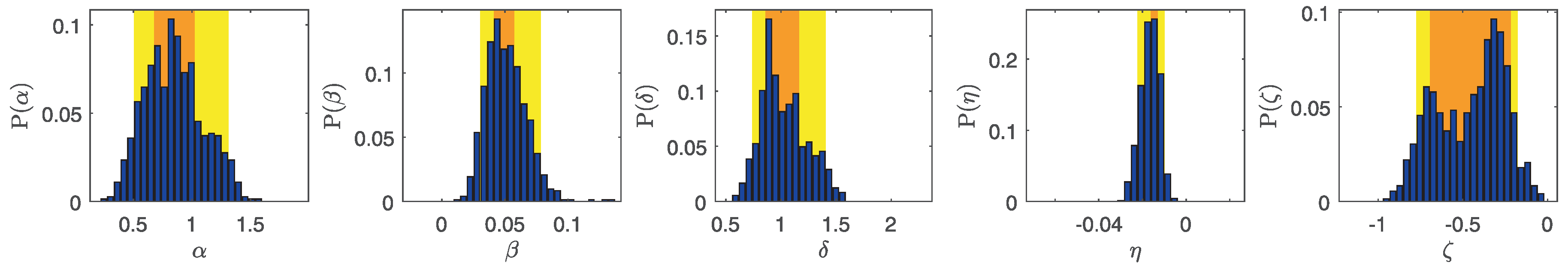
| 0.6365 ± 0.0123 | 0.0411 ± 0.0011 | 0.9379 ± 0.013 | −0.0156 ± 0.0007 | −0.7623 ± 0.0085 | |
| 0.0278 | 0.0478 | 0.051 | 0.0712 | 0.0297 | |
| 0.8501 ± 0.0288 | 0.0465 ± 0.0027 | 0.9206 ± 0.0303 | −0.0130 ± 0.0015 | −0.2970 ± 0.0199 | |
| 0.1033 | 0.1419 | 0.1653 | 0.2562 | 0.0964 | |
| 0.8871 | 0.0292 | 1.265 | −0.0222 | −0.3936 | |
| 0.9752 | 0.0479 | 1.0127 | −0.0192 | −0.5307 | |
| 0.39 | 0.0207 | 0.2576 | 0.0104 | 0.2289 | |
| 0.1521 | 0.0004 | 0.0664 | 0.0001 | 0.0524 | |
| 0.4537 | 0.4338 | 0.6272 | −0.9545 | 0.0224 | |
| 2.3167 | 3.6615 | 3.2615 | 4.3960 | 2.1279 | |
| [0.3901, 1.6716] | [0.016, 0.08] | [0.6261, 1.4316] | [−0.0354, −0.0024] | [−0.8644, −0.1665] | |
| [0.4886, 1.0555] | [0.032, 0.0594] | [0.782, 1.0938] | [−0.0196, −0.009] | [−0.7793, −0.2687] |
© 2018 by the authors. Licensee MDPI, Basel, Switzerland. This article is an open access article distributed under the terms and conditions of the Creative Commons Attribution (CC BY) license (http://creativecommons.org/licenses/by/4.0/).
Share and Cite
Wawrzynczak, A.; Kopka, P. Approximate Bayesian Computation for Estimating Parameters of Data-Consistent Forbush Decrease Model. Entropy 2018, 20, 622. https://doi.org/10.3390/e20080622
Wawrzynczak A, Kopka P. Approximate Bayesian Computation for Estimating Parameters of Data-Consistent Forbush Decrease Model. Entropy. 2018; 20(8):622. https://doi.org/10.3390/e20080622
Chicago/Turabian StyleWawrzynczak, Anna, and Piotr Kopka. 2018. "Approximate Bayesian Computation for Estimating Parameters of Data-Consistent Forbush Decrease Model" Entropy 20, no. 8: 622. https://doi.org/10.3390/e20080622
APA StyleWawrzynczak, A., & Kopka, P. (2018). Approximate Bayesian Computation for Estimating Parameters of Data-Consistent Forbush Decrease Model. Entropy, 20(8), 622. https://doi.org/10.3390/e20080622