SU(2) Decomposition for the Quantum Information Dynamics in 2d-Partite Two-Level Quantum Systems


Abstract
1. Introduction
2. Generalized Hamiltonian
3. Decomposition Generalities
4. GBS: A Non-Local Basis Fitting in {}
4.1. GBS Basis and Hamiltonian Components
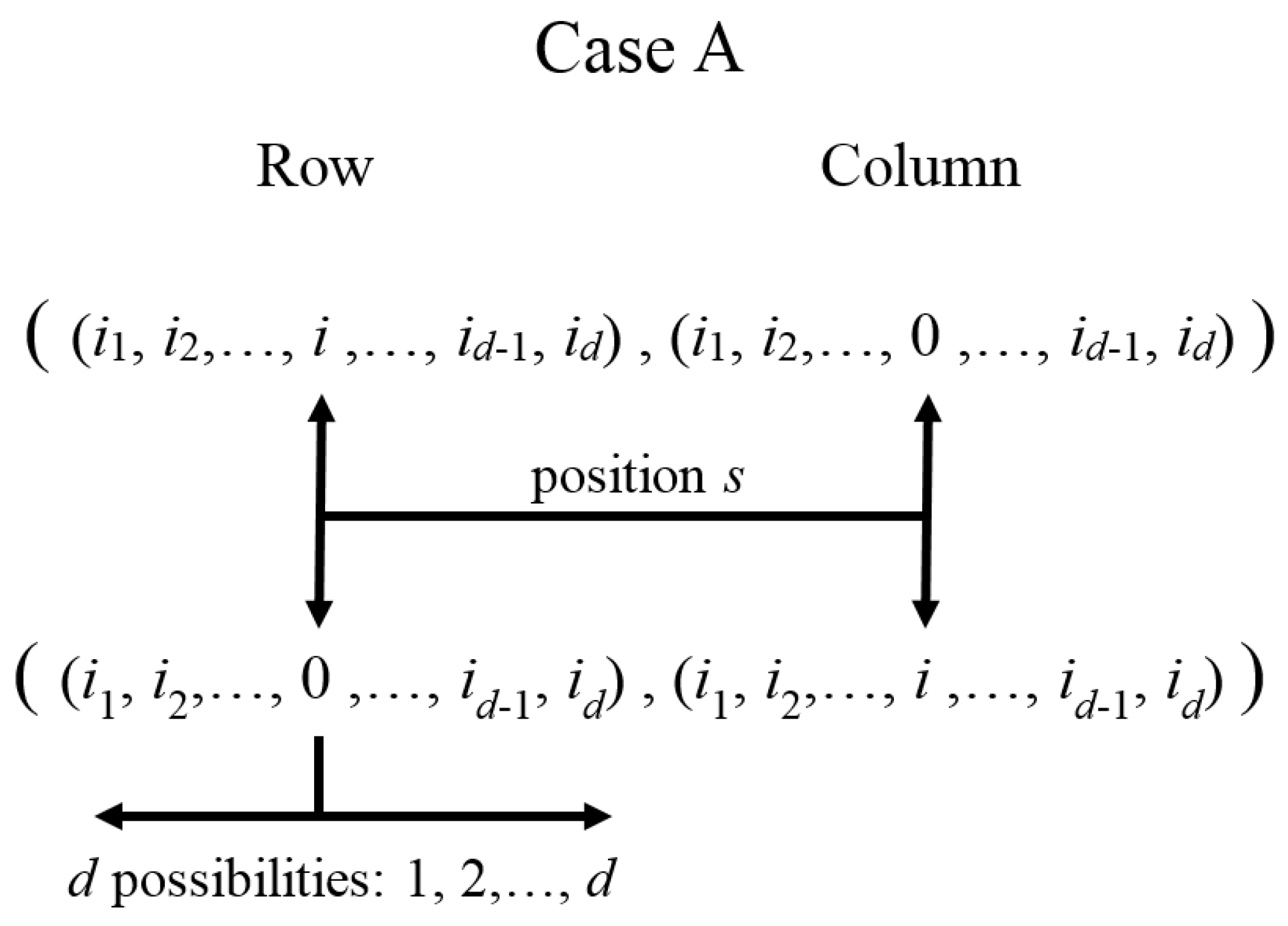
4.2. Case
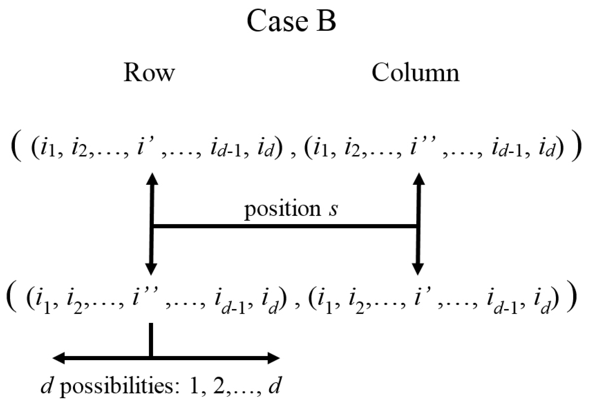
4.3. Case
4.3.1. Analysis of
4.3.2. Analysis of
4.3.3. Analysis of
4.3.4. Analysis of
4.4. Explicit Analytical Formulas for Hamiltonian Components
5. Specific Interactions Generating Decomposition
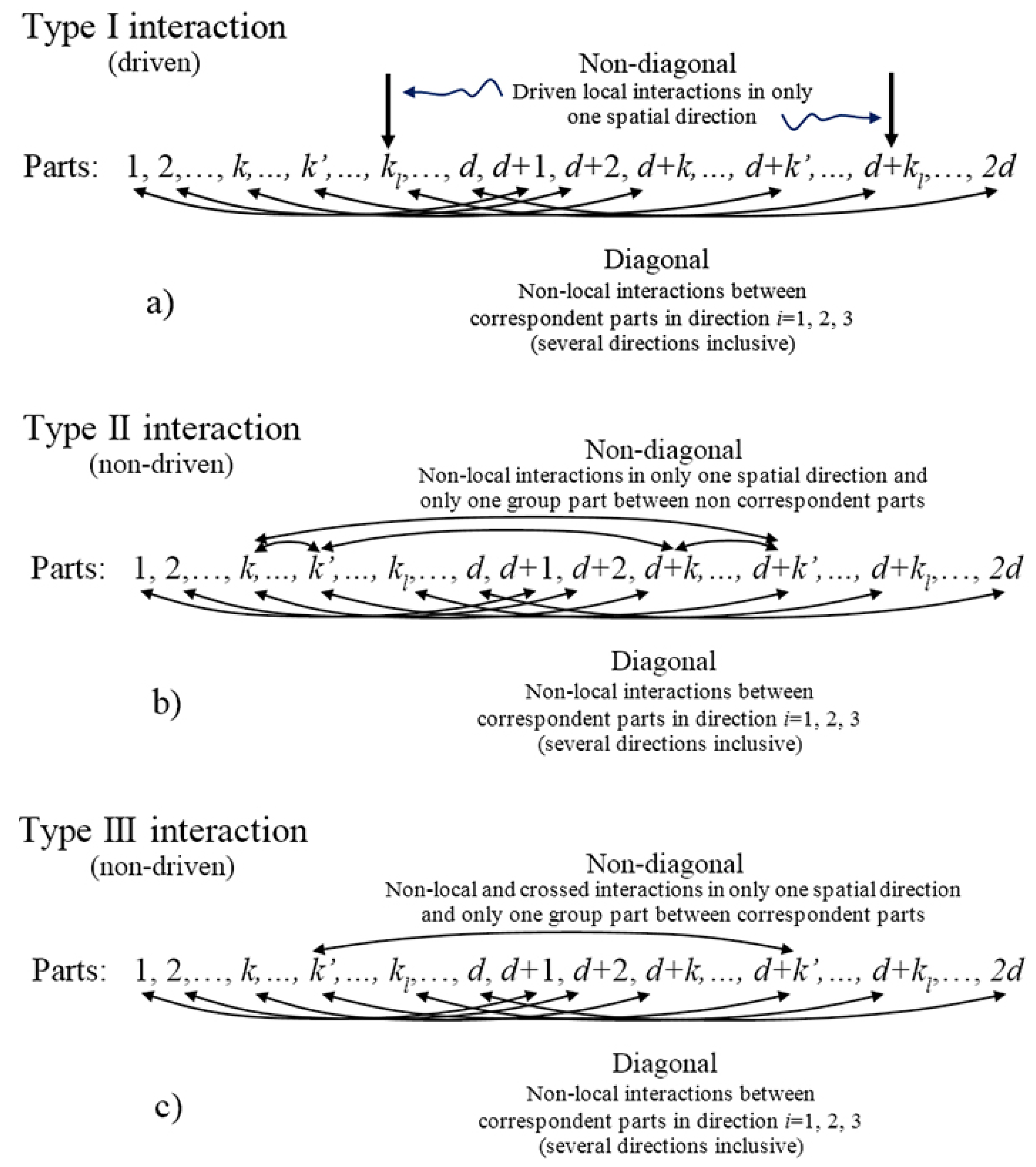
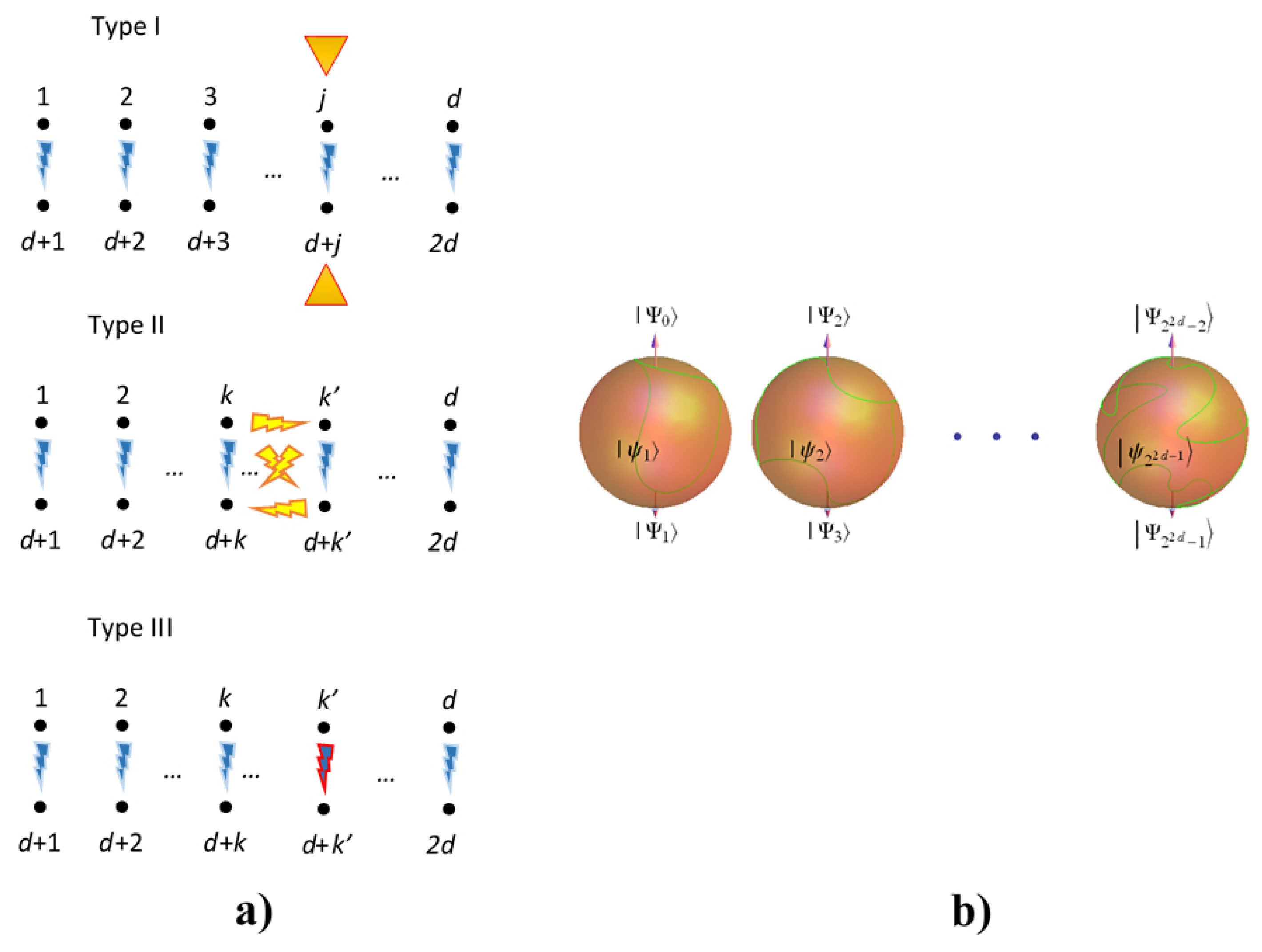
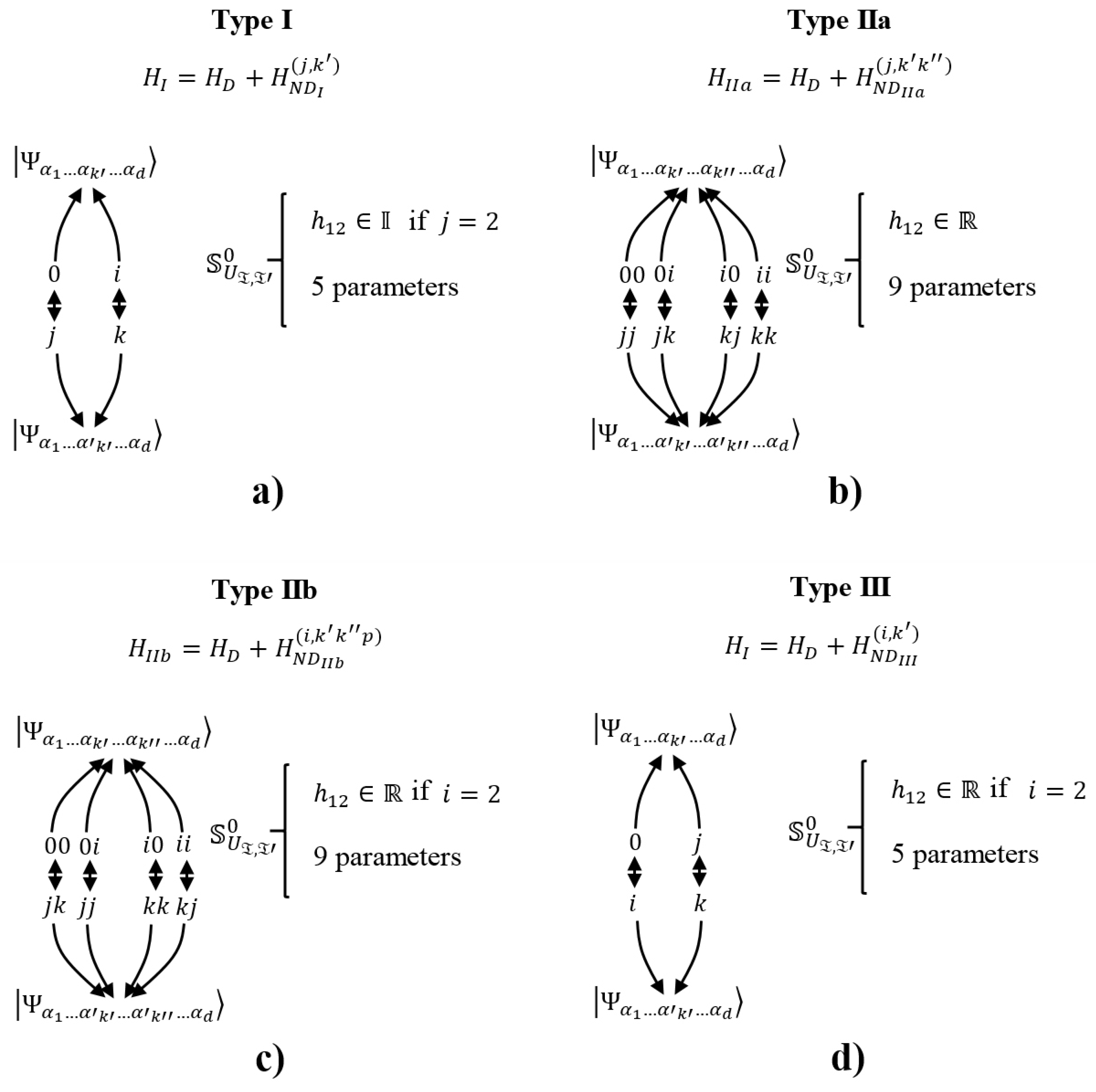
5.1. General Depiction of Interactions Having Decomposition for the GBS Basis
- A:
- Curved arrows point out those qubits related through entangling operations in any case.
- B:
- All curved arrows in the bottom refer to Heisenberg–Ising-like (non-crossed) interactions involving the three possible spatial directions together. Those interaction relations set the correspondent pairs.
- C:
- For the curved arrows in the top, two kinds of entangling operations can be considered according to the text: Heisenberg–Ising-like (non-crossed) interactions or Dzyaloshinskii–Moriya-like (crossed) interactions. Only one characteristic spatial direction is allowed.
- D:
- Type II interactions can be split into Type IIa and Type IIb if interactions in the top are non-crossed or crossed (between parts of two different correspondent pairs), respectively. Type IIb interactions in the top admits only one possible parity from the two possible.
- E:
- Type III interactions admit only crossed interactions in the top between parts of one specific correspondent pair, but the two possible parities together are allowed.
- F:
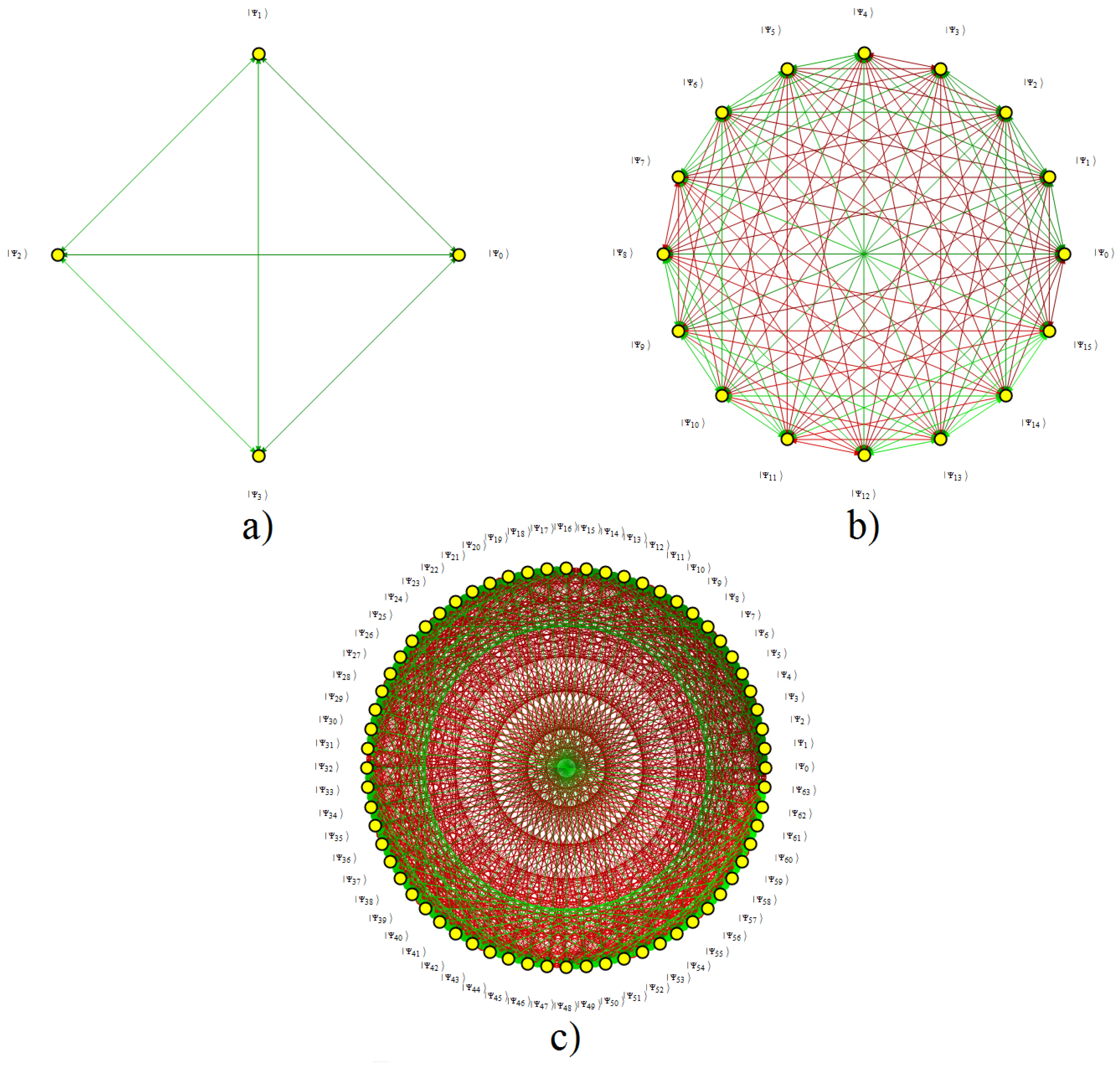
- For Figure 3a, the right arrows correspond to external local interactions such as those generated by magnetic fields on spin-based qubits. Due to their locality, they are referred to as driven interactions, although it actually depends on the available control of the interactions.
5.2. General Structure of Blocks
5.3. Structure of Blocks for Each Interaction
5.3.1. Blocks in Type I Interaction
5.3.2. Blocks in Type II Interaction
5.3.3. Blocks in Type III Interaction
5.4. Available Parameters and Structure of Entries
5.4.1. Structure of Diagonal Entries Belonging to a Specific Block
5.4.2. Structure of Diagonal-Off Entries Belonging to a Specific Block
5.4.3. Block Entries of
5.4.4. Block Entries of
5.4.5. Block Entries of
5.4.6. Block Entries of
6. Connectedness, Superposition, Entanglement and Separability
6.1. Exchange Connectedness under Interactions
6.2. Notable Quantum Processing Operations Achievable under Decomposition
6.3. Decomposition in the Context of Qubit Controlled Gates
6.4. Generating Superposition and Entanglement
6.4.1. Generating Separable Superposition
6.4.2. Entanglement Dynamics under Interactions
6.4.3. Generating Larger Maximal Entangled Systems
6.4.4. Recursive Generation of Larger Maximal Entangled Systems
6.5. Multipartite Entanglement and General States
7. Conclusions
Funding
Acknowledgments
Conflicts of Interest
Appendix A
Appendix A.1. Generic Hamiltonian Expressed in Terms of Pauli Operators
Appendix A.2. Group Theory Basics in the Context of the SU(2) Decomposition
Appendix A.3. Generalized Bell States Basis in Context
Appendix A.4. Illustrative Examples of SU(2) Decomposition
Appendix A.4.1. Case d = 1
Appendix A.4.2. Case d = 2
References
- Feynman, R.P. Simulating Physics with Computers. Int. J. Theor. Phys. 1982, 21, 467–488. [Google Scholar] [CrossRef]
- Deutsch, D. Quantum theory, the Church-Turing principle and the universal quantum computer. Proc. R. Soc. Lond. A 1985, 400, 97–117. [Google Scholar] [CrossRef]
- Steane, A. Error Correcting Codes in Quantum Theory. Phys. Rev. Lett. 1996, 77, 793–797. [Google Scholar] [CrossRef] [PubMed]
- Bennett, C.H.; Brassard, G. Quantum cryptography: Public key distribution and coin tossing. In Proceedings of the International Conference on Computers, Systems & Signal Processing, Bangalore, India, 9–12 December 1984; IEEE: New York, NY, USA, 1984; pp. 175–179. [Google Scholar]
- Ekert, A. Quantum cryptography based on Bell’s theorem. Phys. Rev. Lett. 1991, 67, 661–663. [Google Scholar] [CrossRef] [PubMed]
- Hillery, M.; Vladimír, B.; Berthiaume, A. Quantum secret sharing. Phys. Rev. A 1999, 59, 1829–1834. [Google Scholar] [CrossRef]
- Long, G.; Liu, X. Theoretically efficient high-capacity quantum-key-distribution scheme. Phys. Rev. A 2002, 65, 032302. [Google Scholar] [CrossRef]
- Deng, F.; Long, G.; Liu, X. Two-step quantum direct communication protocol using the Einstein-Podolsky-Rosen pair block. Phys. Rev. A 2003, 68, 042317. [Google Scholar] [CrossRef]
- D’Alessandro, D.; Dahleh, M. Optimal control of two-level quantum systems. IEEE Trans. Autom. Control 2001, 46, 866–876. [Google Scholar] [CrossRef]
- Boscain, U.; Mason, P. Time minimal trajectories for a spin 1/2 particle in a magnetic field. J. Math. Phys. 2006, 47, 062101. [Google Scholar] [CrossRef]
- Delgado, F. Algebraic and group structure for bipartite anisotropic Ising model on a non-local basis. Int. J. Quantum Inf. 2015, 13, 1550055. [Google Scholar] [CrossRef]
- Delgado, F. Generation of non-local evolution loops and exchange operations for quantum control in three dimensional anisotropic Ising model. ArXiv, 2016; arXiv:1410.5515. [Google Scholar]
- Delgado, F. Stability of Quantum Loops and Exchange Operations in the Construction of Quantum Computation Gates. J. Phys. 2016, 648, 012024. [Google Scholar]
- McConnell, R.; Bruzewicz, C.; Chiaverini, J.; Sage, J. Characterization and Mitigation of Anomalous Motional Heating in Surface-Electrode Ion Traps. In Proceedings of the 46th Annual Meeting of the APS Division of Atomic, Molecular and Optical Physics, Columbus, OH, USA, 8–12 June 2015; Volume 60. [Google Scholar]
- Gambetta, J.M.; Jerry, M.; Steffen, M. Building logical qubits in a superconducting quantum computing system. npj Quantum Inf. 2017, 3, 1–7. [Google Scholar] [CrossRef]
- Fubini, A.; Roscilde, T.; Tognetti, V.; Tusa, M.; Verrucchi, P. Reading entanglement in terms of spin-configuration in quantum magnet. Eur. Phys. J. D 2006, 38, 563–570. [Google Scholar] [CrossRef]
- Pfaff, W.; Taminiau, T.; Robledo, L.; Bernien, H.; Matthew, M.; Twitchen, D.; Hanson, R. Demonstration of entanglement-by-measurement of solid-state qubits. Nat. Phys. 2013, 9, 29–33. [Google Scholar] [CrossRef]
- Magazzu, L.; Jamarillo, J.; Talkner, P.; Hanggi, P. Generation and stabilization of Bell states via repeated projective measurements on a driven ancilla qubit. ArXiv, 2018; arXiv:1802.04839v1. [Google Scholar]
- Nielsen, M.; Chuang, I. Quantum Computation and Quantum Information; Cambridge University Press: Cambridge, UK, 2011. [Google Scholar]
- Lieb, E.; Schultz, T.; Mattis, D. Two soluble models of an antiferromagnetic chain. Ann. Phys. 1961, 16, 407–466. [Google Scholar] [CrossRef]
- Baxter, R.J. Exactly Solved Models in Statistical Mechanics; Academic Press: New York, NY, USA, 1982. [Google Scholar]
- Sych, D.; Leuchs, G. A complete basis of generalized Bell states. New J. Phys. 2009, 11, 013006. [Google Scholar] [CrossRef]
- Delgado, F. Modeling the dynamics of multipartite quantum systems created departing from two-level systems using general local and non-local interactions. J. Phys. 2017, 936, 012070. [Google Scholar] [CrossRef]
- Dzyaloshinskii, I. A thermodynamic theory of weak ferromagnetism of antiferromagnetics. J. Phys. Chem. Solids 1958, 4, 241–255. [Google Scholar] [CrossRef]
- Moriya, T. Anisotropic Superexchange Interaction and Weak Ferromagnetism. Phys. Rev. 1960, 120, 91–98. [Google Scholar] [CrossRef]
- Delgado, F. Two-qubit quantum gates construction via unitary factorization. Quantum Inf. Comput. 2017, 17, 721–746. [Google Scholar]
- Delgado, F. Generalized Bell states map physical systems’ quantum evolution into a grammar for quantum information processing. J. Phys. 2017, 936, 012083. [Google Scholar] [CrossRef]
- Uhlmann, A. Anti-(conjugate) linearity. Sci. China Phys. Mech. Astron. 2016, 59, 630301. [Google Scholar] [CrossRef]
- Boykin, P.; Mor, T.; Pulver, M.; Roychowdhury, V.; Vatan, F. On universal and fault tolerant quantum computing. ArXiv, 1999; arXiv:9906054. [Google Scholar]
- Li, C.; Jones, R.; Yin, X. Decomposition of unitary matrices and quantum gates. Int. J. Quantum Inf. 2013, 11, 1350015. [Google Scholar] [CrossRef]
- Delgado, F. Universal Quantum Gates for Quantum Computation on Magnetic Systems Ruled by Heisenberg-Ising Interactions. J. Phys. 2017, 839, 012014. [Google Scholar] [CrossRef]
- Barenco, A.; Bennett, C.; Cleve, R.; DiVincenzo, D.; Margolus, N.; Shor, P.; Sleator, T.; Smolin, J.; Weinfurter, H. Elementary gates for quantum computation. Phys. Rev. A 1995, 52, 3457. [Google Scholar] [CrossRef] [PubMed]
- Liu, Y.; Long, G.; Sun, Y. Analytic one-bit and CNOT gate constructions of general n-qubit controlled gates. Int. J. Quantum Inf. 2008, 6, 447–462. [Google Scholar] [CrossRef]
- Hou, S.; Wang, L.; Yi, X. Realization of quantum gates by Lyapunov control. Phys. Lett. A 2014, 378, 699–704. [Google Scholar] [CrossRef]
- Gurvits, L. Classical complexity and quantum entanglement. J. Comput. Syst. Sci. 2004, 69, 448–484. [Google Scholar] [CrossRef]
- Uhlmann, A. Fidelity and concurrence of conjugated states. Phys. Rev. A 2000, 62, 032307. [Google Scholar] [CrossRef]
- Serikawa, T.; Shiozawa, Y.; Ogawa, H.; Takanashi, N.; Takeda, S.; Yoshikawa, J.; Furusawa, A. Quantum information processing with a travelling wave of light. In Proceedings of the SPIE-OPTO, San Francisco, CA, USA, 19–23 August 2018. [Google Scholar]
- Britton, J.; Sawyer, B.; Keith, A.; Wang, J.; Freericks, J.; Uys, H.; Biercuk, M.; Bollinger, J. Engineered two-dimensional Ising interactions in a trapped-ion quantum simulator with hundreds of spins. Nature 2012, 484, 489–492. [Google Scholar] [CrossRef] [PubMed]
- Bohnet, J.; Sawyer, B.; Britton, J.; Wall, M.; Rey, A.; Foss-Feig, M.; Bollinger, J. Quantum spin dynamics and entanglement generation with hundreds of trapped ions. Science 2016, 352, 1297–1301. [Google Scholar] [CrossRef] [PubMed]
- De Sa Neto, O.; de Oliveira, M. Hybrid Qubit gates in circuit QED: A scheme for quantum bit encoding and information processing. ArXiv, 2011; arXiv:1110.1355. [Google Scholar]
- Delgado, F.; Rodríguez, S. Modeling quantum information dynamics achieved with time-dependent driven fields in the context of universal quantum processing. ArXiv, 2018; arXiv:1805.05477. [Google Scholar]
- Hall, B. Lie Groups, Lie Algebras, and Representations: An Elementary Introduction; Graduate Texts in Mathematics 222; Springer: Cham, Switzerland, 2015. [Google Scholar]
- Hall, B. An Elementary Introduction to Groups and Representations. ArXiv, 2000; arXiv:quant-ph/0005032. [Google Scholar]


| Basis Arrangement | Hamiltonian |
|---|---|
| Hamiltonian | Entries Type | Entries by Column/Row | Parameters by Entry |
|---|---|---|---|
| Diagonal | 1 | ||
| Non-diagonal | d | 2 | |
| Diagonal | 1 | d | |
| Non-diagonal | 4 | ||
| Non-diagonal | d | 2 | |
| Non-diagonal | 4 | ||
| 2 × 2 block | 2 | ||
| 2 × 2 block | 2 | ||
| 2 × 2 block | 2 |
| i | i | |||||||
| i | i | |||||||
| 1 | 1 | |||||||
| 1 | 1 | |||||||
| i | ||||||||
| i | ||||||||
| 1 | 1 | |||||||
| 1 | 1 | 1 | 1 |
| Case | S | |
|---|---|---|
| (a) | 1 | |
| (b) | ||
| (c) | 0 | |
| (d) | ||
| (e) |
© 2018 by the author. Licensee MDPI, Basel, Switzerland. This article is an open access article distributed under the terms and conditions of the Creative Commons Attribution (CC BY) license (http://creativecommons.org/licenses/by/4.0/).
Share and Cite
Delgado, F. SU(2) Decomposition for the Quantum Information Dynamics in 2d-Partite Two-Level Quantum Systems. Entropy 2018, 20, 610. https://doi.org/10.3390/e20080610
Delgado F. SU(2) Decomposition for the Quantum Information Dynamics in 2d-Partite Two-Level Quantum Systems. Entropy. 2018; 20(8):610. https://doi.org/10.3390/e20080610
Chicago/Turabian StyleDelgado, Francisco. 2018. "SU(2) Decomposition for the Quantum Information Dynamics in 2d-Partite Two-Level Quantum Systems" Entropy 20, no. 8: 610. https://doi.org/10.3390/e20080610
APA StyleDelgado, F. (2018). SU(2) Decomposition for the Quantum Information Dynamics in 2d-Partite Two-Level Quantum Systems. Entropy, 20(8), 610. https://doi.org/10.3390/e20080610