5.1. A Detection Example for
In this subsection, suppose that
and
The corresponding decision function is
When we add an additive noise
to
, the noise modified decision function can be written as
It is obvious from (27) that the detection performance obtained by setting the threshold as
and adding a noise
is identical with that achieved by keeping the threshold as zero and adding a noise
. As a result, the optimal noise enhanced performances obtained are the same for different thresholds. That is also to say, the randomization between different thresholds cannot improve the optimum performance further and only the non-randomization case should be considered in this example. According to (8), we have
where
. Based on the analysis on Equation (8), the original false-alarm and detection probabilities are
and
, respectively.
From the definition of function
,
, and
are monotonically increasing with
and
for any
. In addition, both
and
are one-to-one mapping functions w.r.t.
. Therefore, we have
and
for any
. Furthermore,
and
. The relationship between
and
is one-to-one, as well as that between
and
. As a result,
,
,
, and
for any
. That is to say,
and
, where
and
are the respective optimal noise components for case (i) and case (ii) for any
. From [
2,
24], we have
Then the pdf of the optimal additive noise corresponding to case (i) and case (ii) for the detector given in (26) can be expressed as
where
and
. Thus the suitable additive noise for case (iii) can be given by
where
. In this example, let
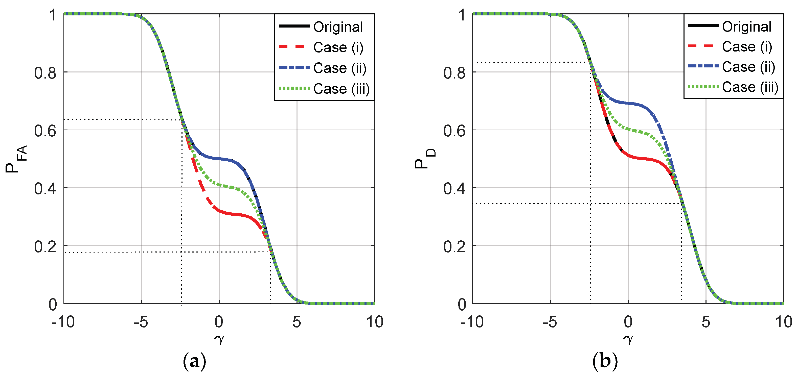
. The false alarm and detection probabilities for the three cases versus different
are shown in
Figure 1.
As plotted in
Figure 1, with the increase of
, the false alarm and detection probabilities for the three cases and the original detector gradually decrease from 1 to 0, and the noise enhanced phenomenon only occurs when
. Namely, the detection performance can be improved by adding additive noise when the value of
is between −2.5 and 3.5. When
,
and
, the corresponding
and
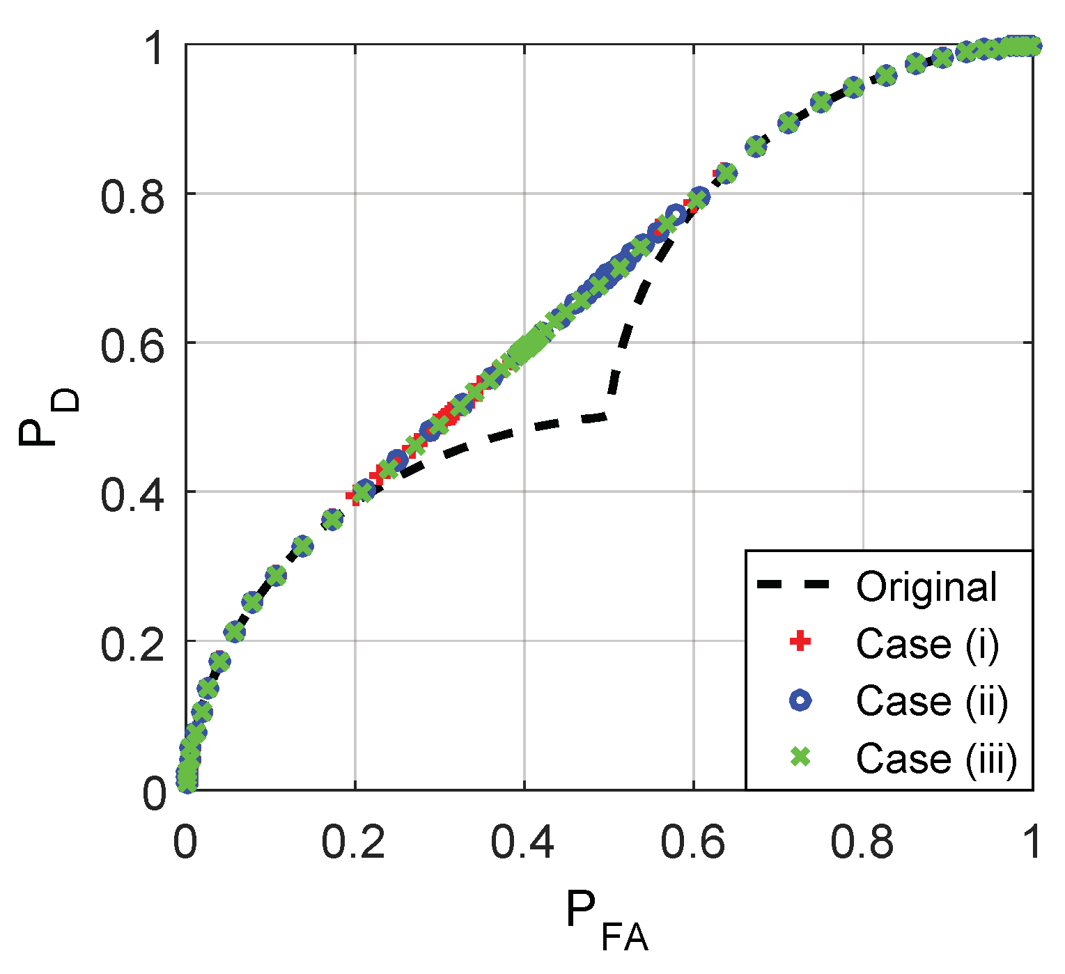
, thereby the additive noises as shown in (32) and (33) exist to improve the detection performance. Furthermore, the receiver operating characteristic (ROC) curves for the three cases and the original detector are plotted in
Figure 2. The ROC curves for the three cases overlap with each other exactly, and the detection probability can be increased by adding additive noise only when the false-alarm probability is between 0.1543 and 0.6543.
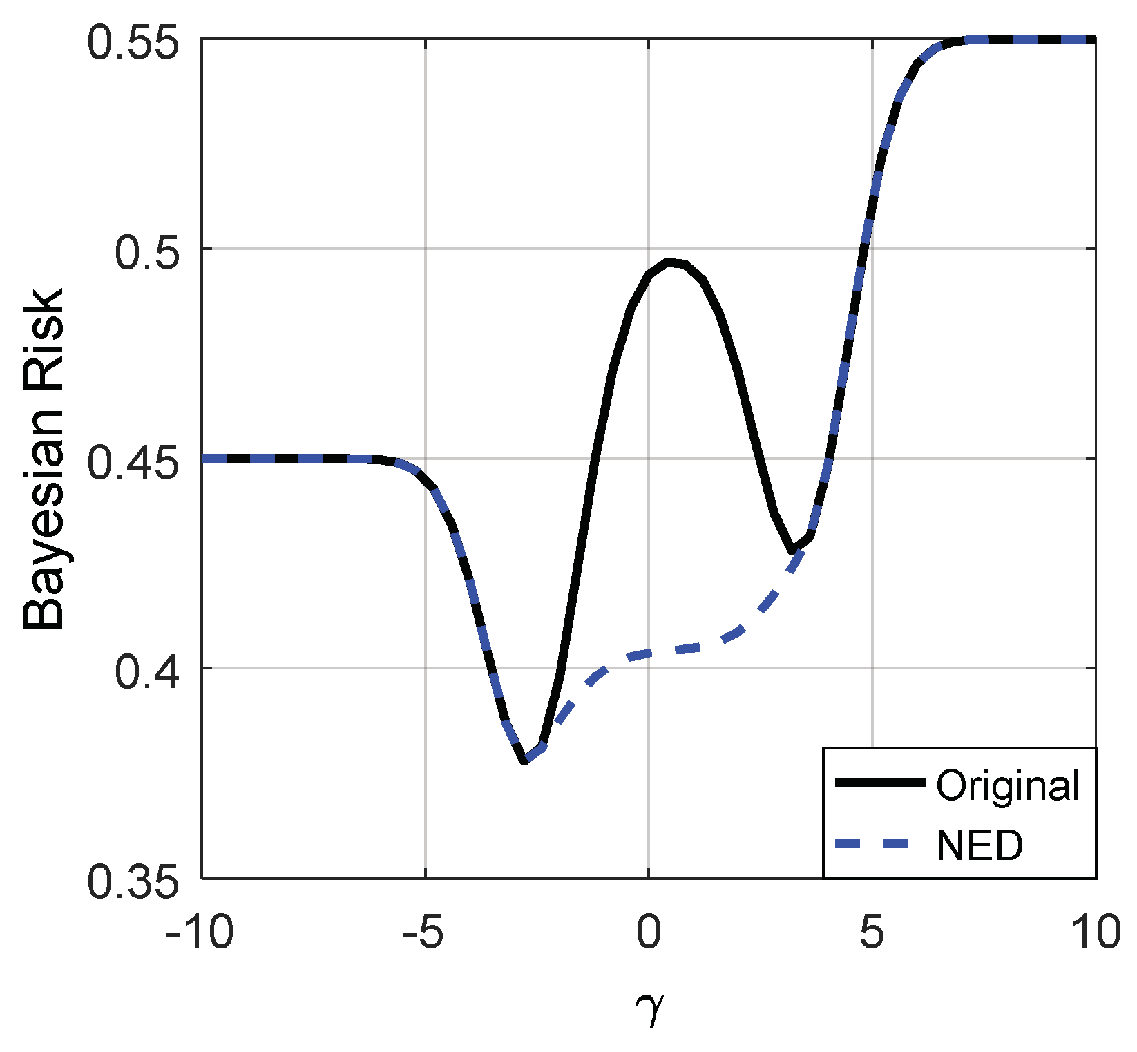
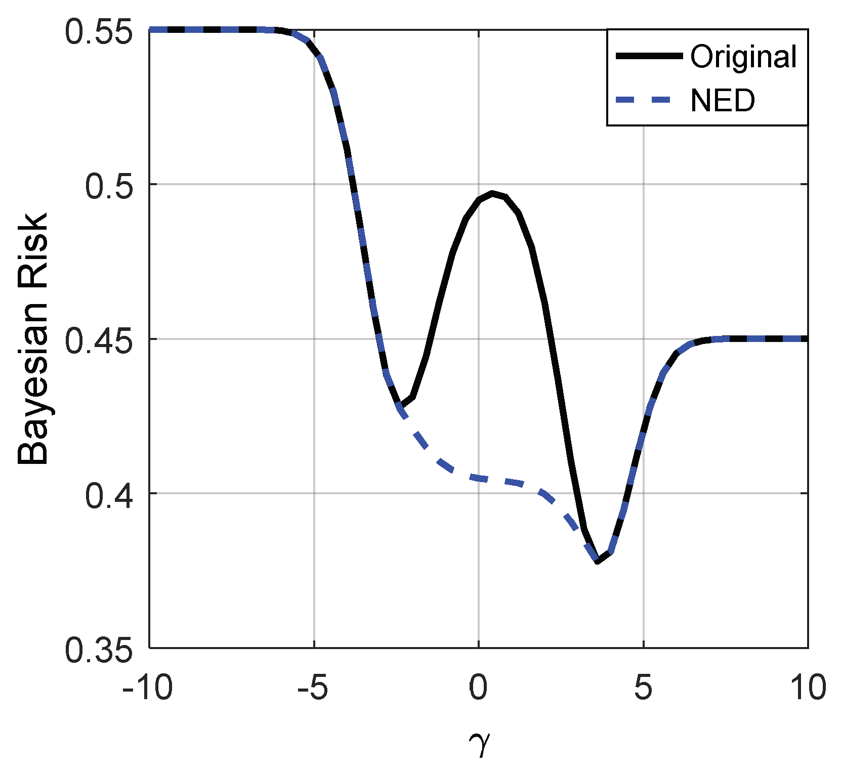
Given
and the prior probability
,
, the noise enhanced Bayes risk obtained according to case (iii) is given by
where
and
. Let
,
and
, then the Bayes risk of the original detector is calculated as
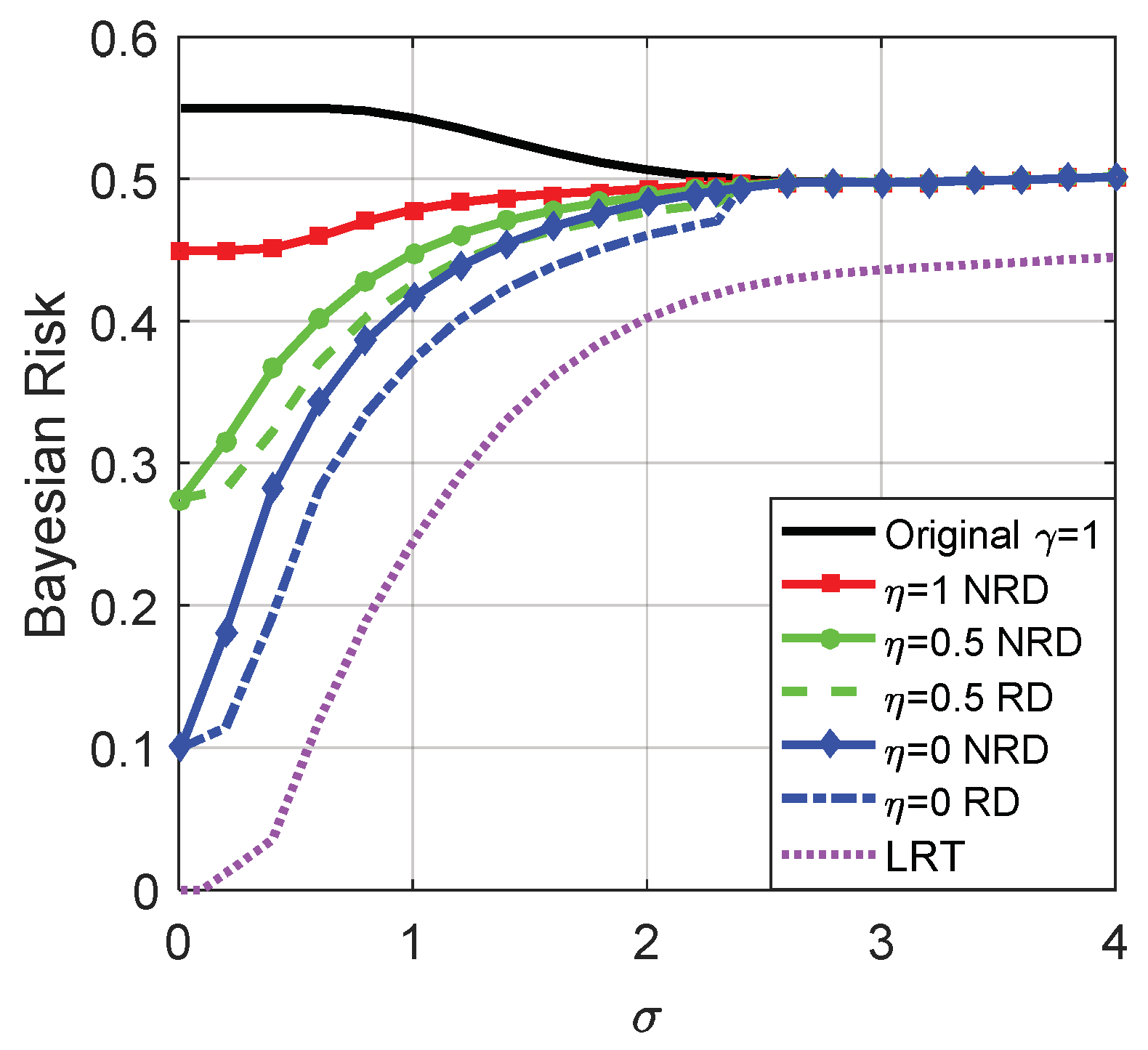
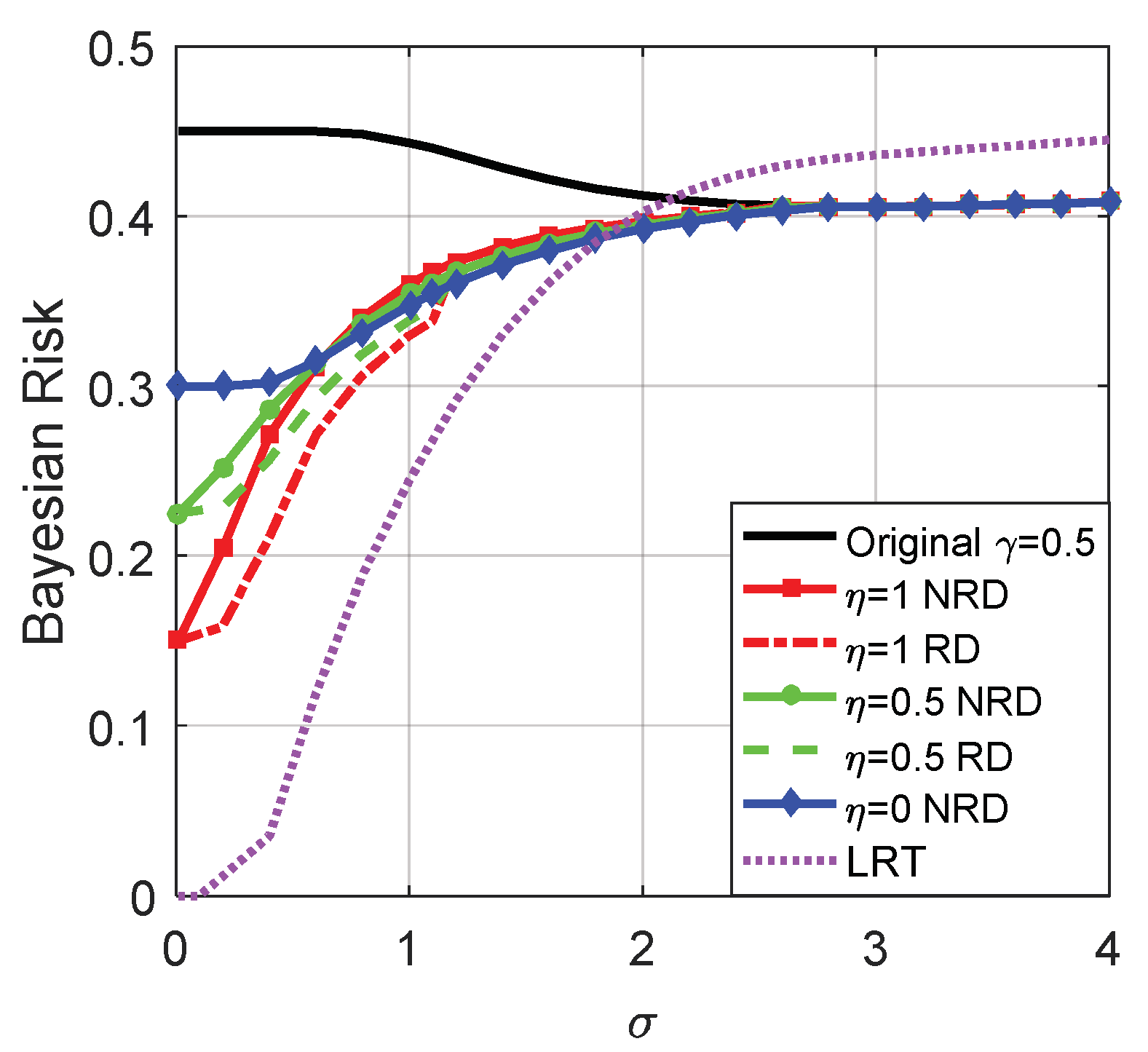
Figure 3 and
Figure 4 depict the Bayes risks of the noise enhanced and the original detectors versus different
for
and 0.55, respectively.
From
Figure 3 and
Figure 4, we can see that when the decision threshold
is very small, the Bayes risks of the noise enhanced and the original detectors are close to
. As illustrated in
Figure 3 and
Figure 4, only when
, can the Bayes risk be decreased by adding additive noise. With the increase of
, the difference between the Bayes risks of the noise enhanced detector and the original detector first increases and then decreases to zero, and reaches the maximum value when
. If the decision threshold
is large enough, the Bayes risks for the two detectors are close to
. In addition, there is no link between the values of
and the possibility of the detection performance can or cannot be improved via additive noise, which is consistent with (35).
5.2. A Detection Example for
In this example, suppose that
where
. When
, we have
It is obvious that
when
and
when
, which implies the detection result is invalid if
or
. In addition, the detection performance is the same for
(
). Therefore, suppose that two alternative thresholds are
and
, the corresponding decision functions are denoted by
and
, respectively. Let
, then we have
where
,
is the decision function given in (26) with
. Based on the theoretical analysis in
Section 4,
, and
. Furthermore,
and
.
Through a series of analyses and calculations, it is true that , where and are determined by and , respectively. Similarly, , where and are determined by and , respectively. Moreover, where .
On the other hand, where and are determined by and . Moreover, , where and . As a consequence, where .
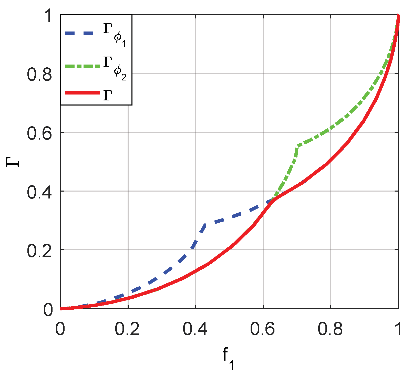
The minimum achievable false-alarm probabilities for
and
, i.e.,
and
, can be obtained, respectively, by utilizing the relationships between
,
, and
as depicted in
Figure 5. Then
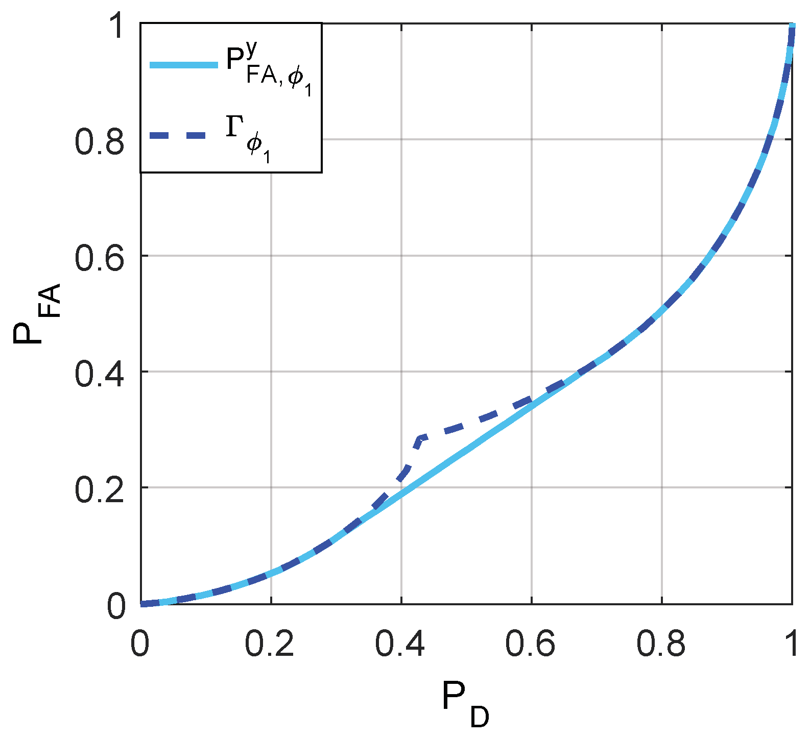
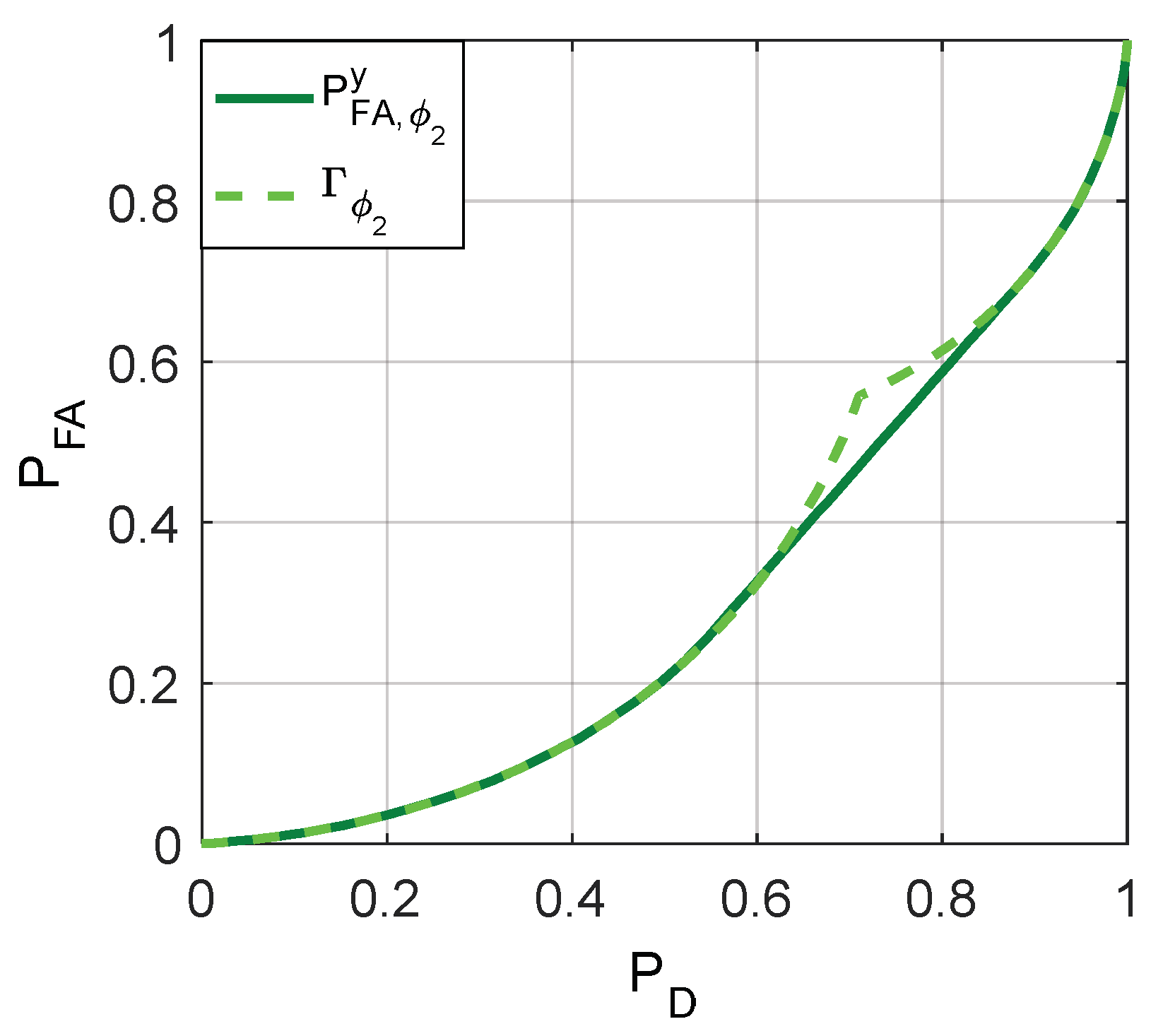
Figure 6,
Figure 7 and
Figure 8 are given to illustrate the relationship between
and
clearly under two different decision thresholds. As illustrated in
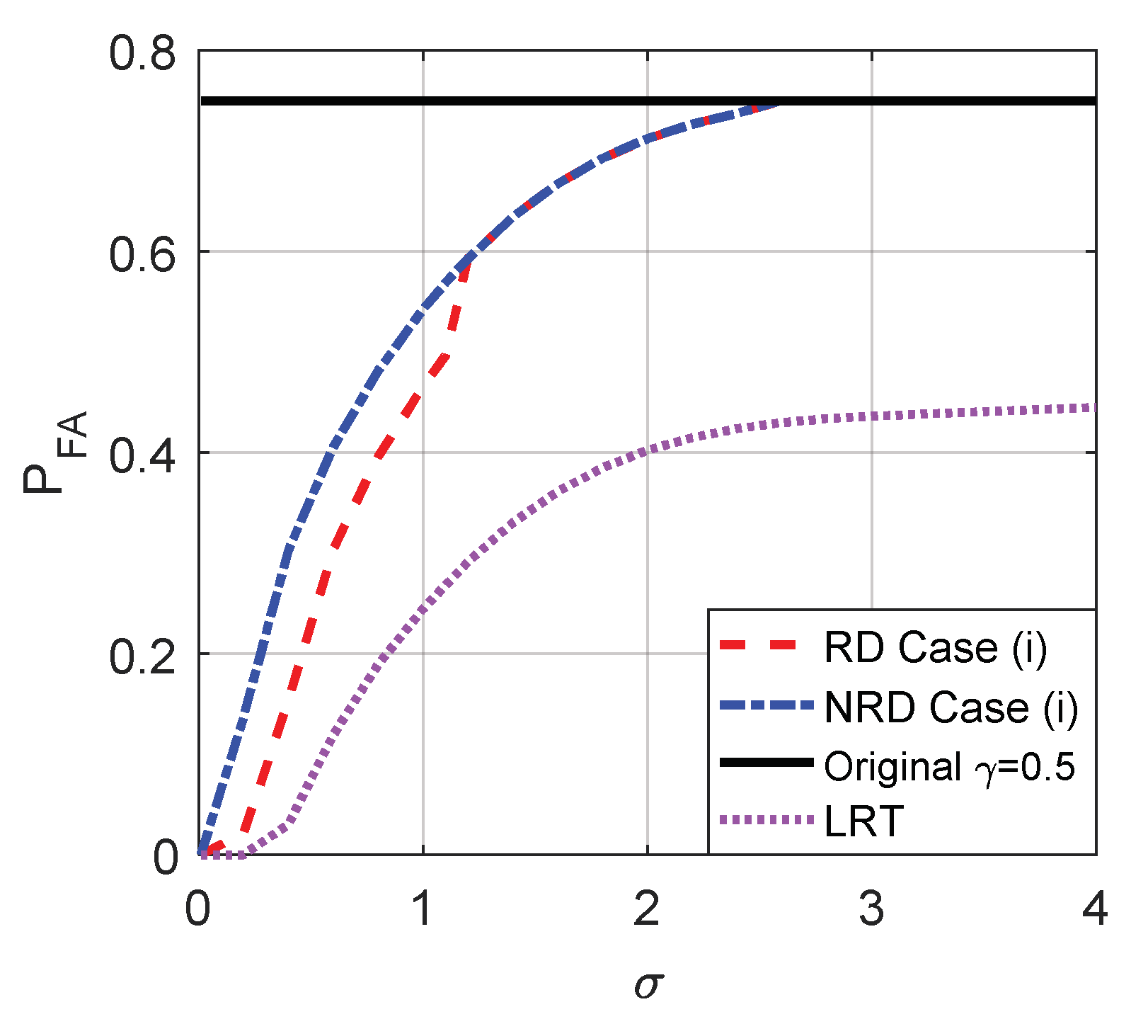
Figure 6, for the case of threshold
, the false-alarm probability can be decreased by adding an additive noise when
. Correspondingly, the false-alarm probability can be decreased by adding an additive noise only when
for
as shown in
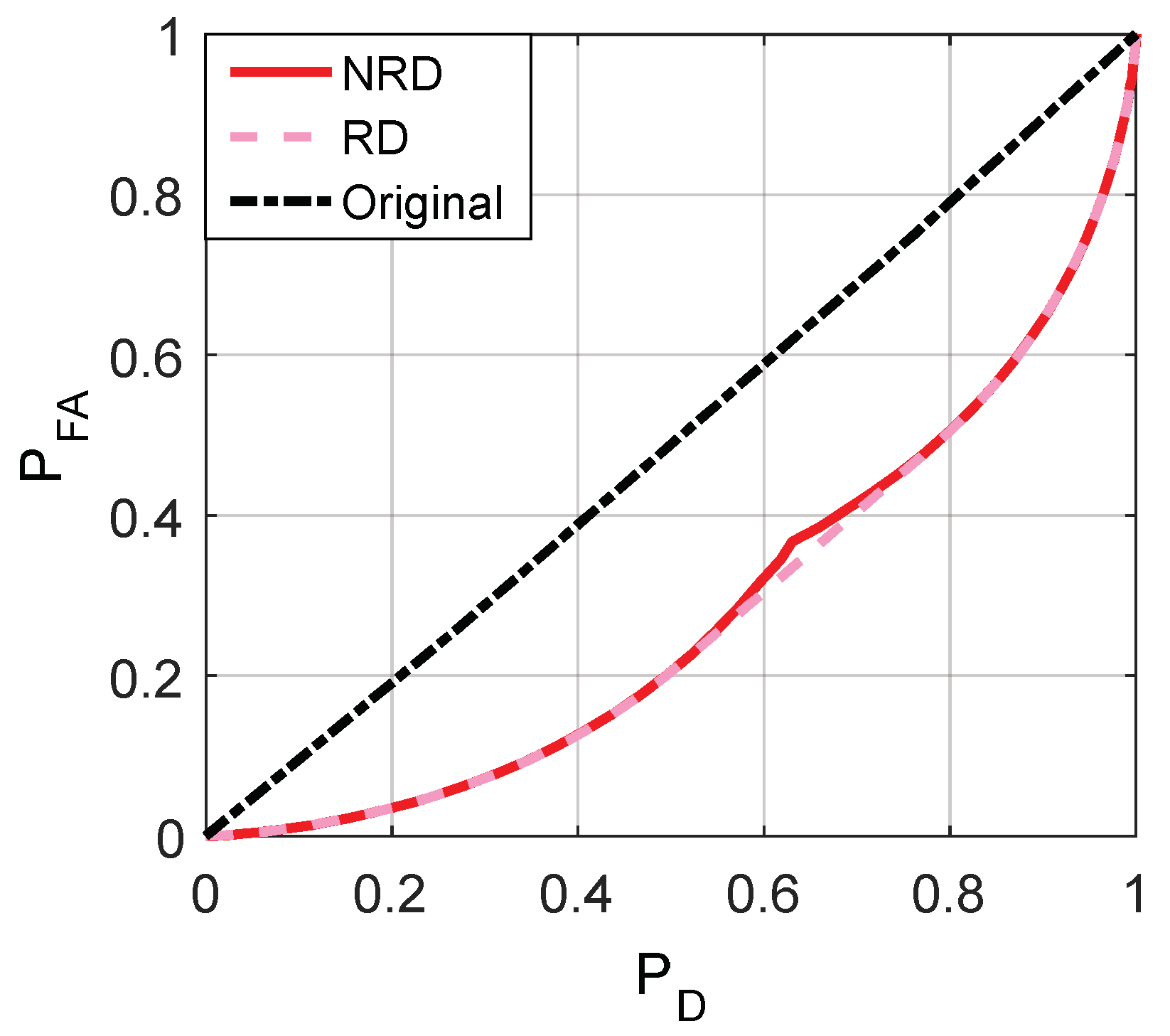
Figure 7. The minimum false-alarm probability for a given
without threshold randomization is
, which is plotted in
Figure 8 and represented by the legend “NRD”.
As illustrated in
Figure 8, when the randomization between decision thresholds is allowed, the noise modified false-alarm probability can be decreased further compared with the case where no randomization between decision thresholds is allowed for
. Actually, the minimum achievable noise modified false-alarm probability is obtained by a suitable randomization between two threshold and discrete vector pairs, i.e.,
and
, with probabilities
and
, respectively, such that
Remarkably, the minimum false-alarm probability obtained in the “NRD” case is always superior to the original false-alarm probability for any .
If the randomization between different decision thresholds is not allowed, the detection probability can be increased by adding additive noise when and for and , respectively. When the randomization is allowed, for , the maximum achievable detection probability can be obtained by a randomization of two pairs and with the corresponding weights and .
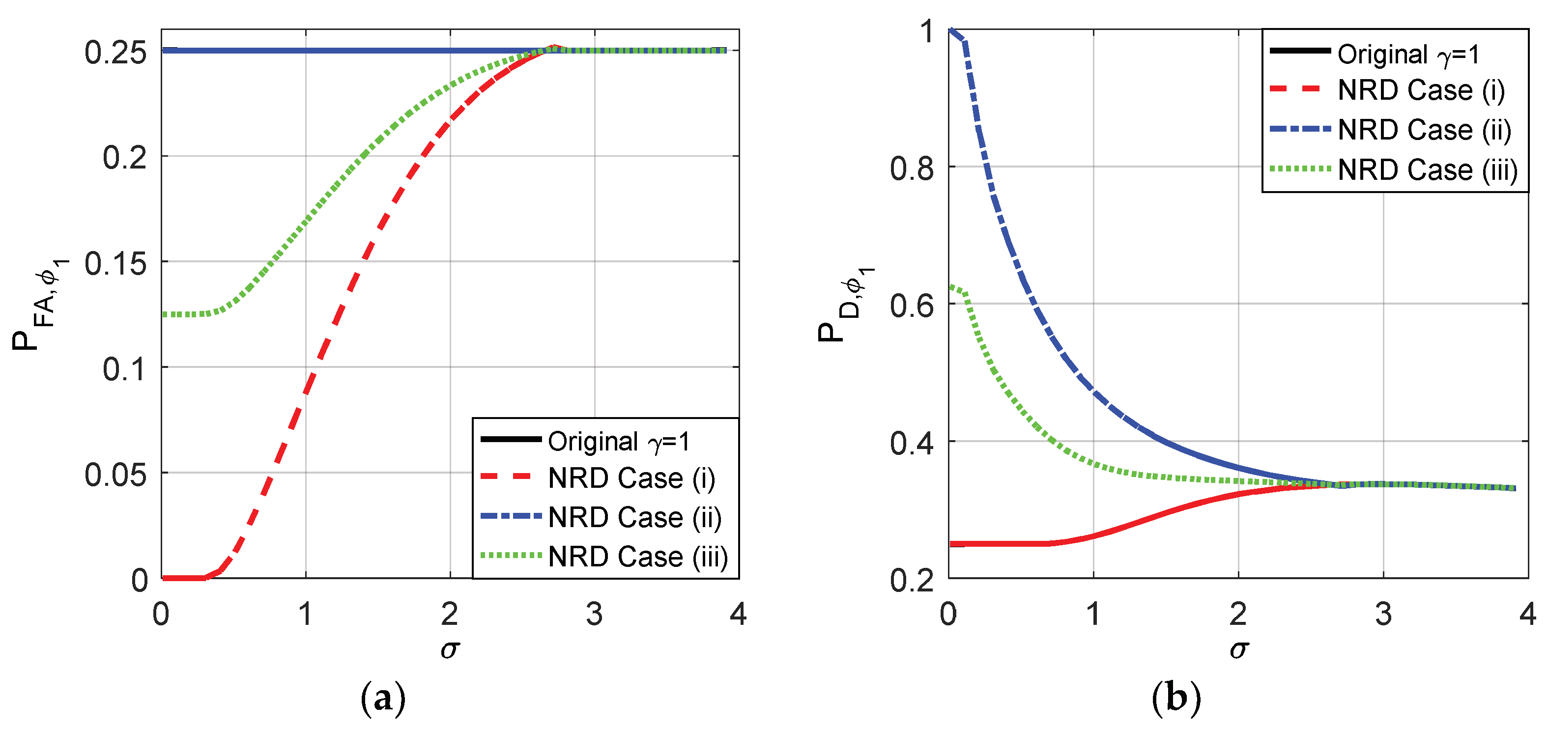
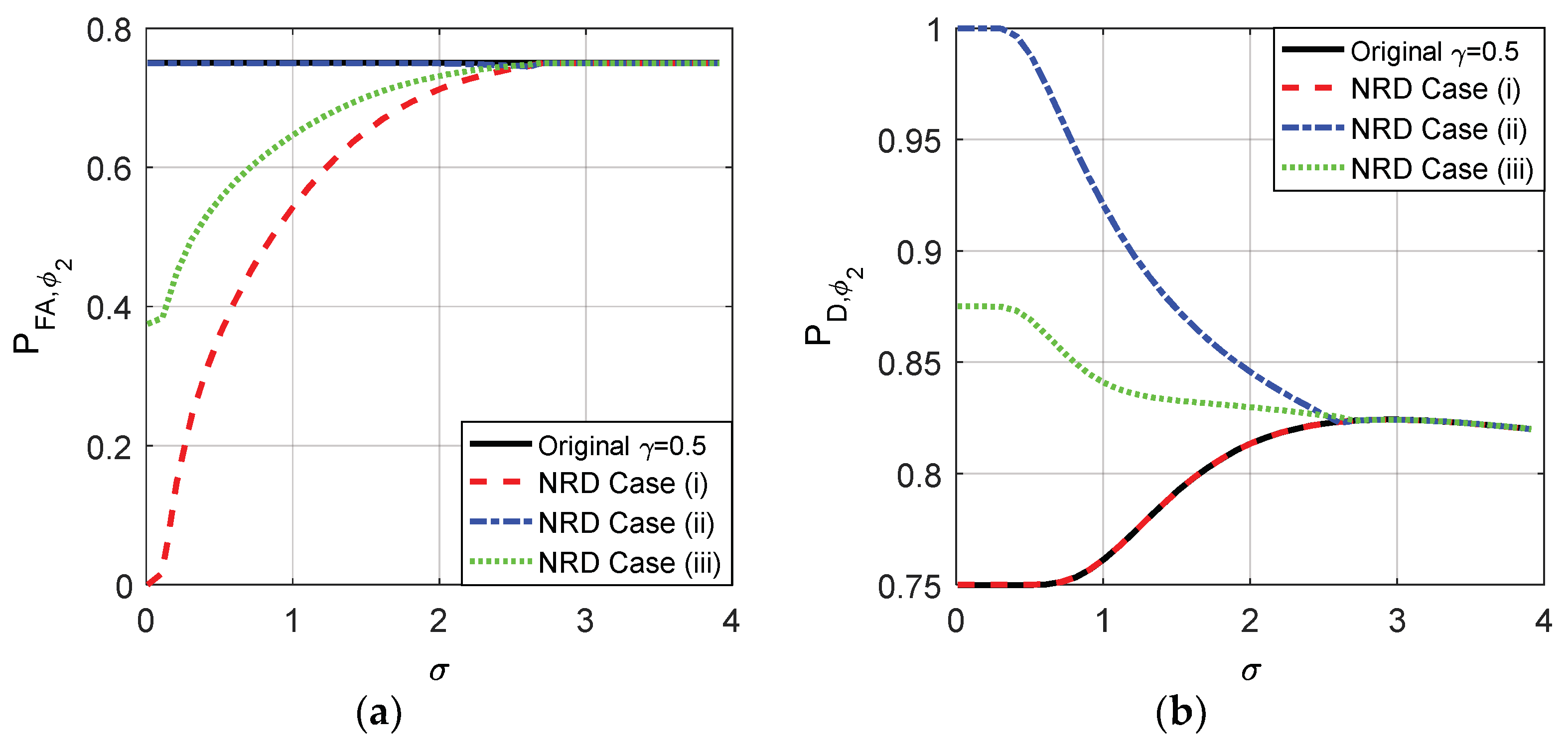
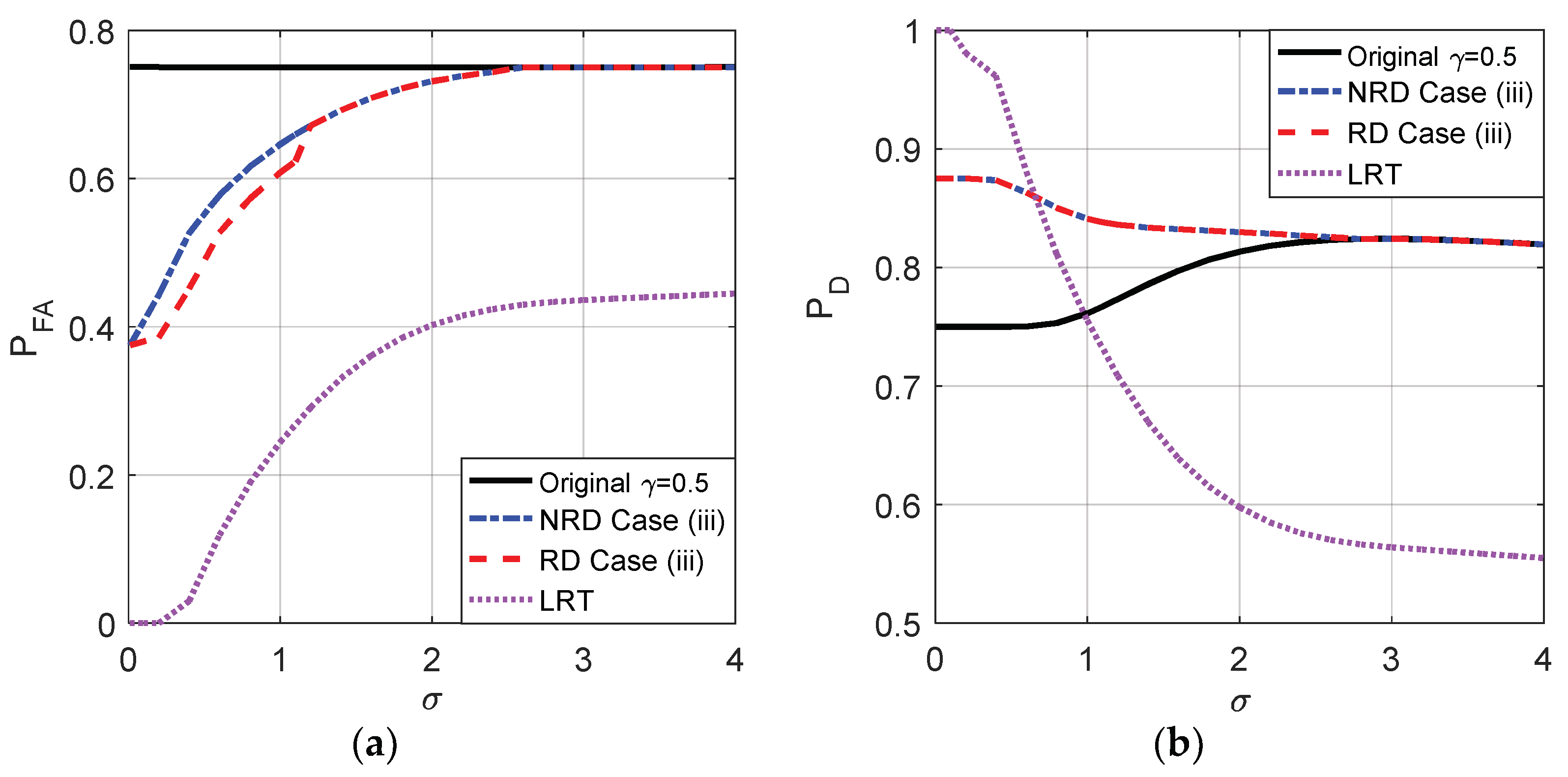
The probabilities of false-alarm and detection for different
of the original detector and cases (i), (ii), and (iii) when the decision threshold
and
are compared in
Figure 9 and
Figure 10, respectively. As shown in
Figure 9a,b, the original
maintains 0.25 for any
and the original
is between 0.25 and 0.3371 when
. As plotted in
Figure 10a,b, the original
maintains 0.75 and the original
is between 0.75 and 0.8242 when
.
According to the analyses above, the original
and
obtained when
and
are in the interval where the noise enhanced detection could occur. When the randomization between the thresholds is not allowed, according to the theoretical analysis, the optimal solutions of the noise enhanced detection performance for both case (i) and (ii) are to choose a suitable threshold and add the corresponding optimal noise to the observation. After some comparisons, the suitable threshold is just the original detector under the constraints in which
and
in this example. Naturally, case (iii) can be achieved by choosing the original detector and adding the noise which is a randomization between two optimal additive noises obtained in case (i) and case (ii). The details are plotted in
Figure 9 and
Figure 10 for the original threshold
and 0.5, respectively.
From
Figure 9 and
Figure 10, it is clear that the smaller the
, the smaller the false-alarm probability and the larger the detection probability. When
is close to 0, the false-alarm probability obtained in case (i) is close to 0 and the detection probability obtained in case (ii) is close to 1. As shown in
Figure 9, compared to the original detector, the noise enhanced false-alarm probability and the detection probability obtained in case (iii) are decreased by 0.125 and increased by 0.35, respectively, when
is close to 0 where
and
. As shown in
Figure 10, compared to the original detector, the noise enhanced false-alarm probability obtained in case (iii) is decreased by 0.375 and the corresponding detection probability is increased by 0.125, respectively, when
and
. With the increase of
, the improvements of false-alarm and detection probabilities decrease gradually to zero as shown in
Figure 9 and
Figure 10. When
, because the pdf of
gradually becomes a unimodal noise, the detection performance cannot be enhanced by adding any noise.
After some calculations, we know that under the constraints that
and
, the false-alarm probability cannot be decreased further by allowing randomization between the two thresholds compared to the non-randomization case when the original threshold is
. It means that even if randomization is allowed, the minimum false-alarm probability in case (i) is obtained by choosing threshold
and adding the corresponding optimal additive noise, and the achievable minimum false-alarm probability in case (i) is the same as that plotted in
Figure 9. On the contrary, the detection probability obtained under the same constraints when randomization exists between different thresholds is greater than that obtained in the non-randomization case for
, which is shown in
Figure 11. Based on the analysis in
Section 3.2, the maximum detection probability in case (ii) can be achieved by a suitable randomization of the two decision thresholds and noise pairs
and
with probabilities
and
, respectively, where
. Such as
,
, and
when
. In addition,
Figure 11 also plots the
under the Likelihood ratio test (LRT) based on the original observation
. It is obvious that the
obtained under LRT is superior to that obtained in case (ii) for each
. Although the performance of LRT is much better than the original and noise enhanced decision solutions, its implementation is much more complicated.
Naturally, case (iii) can also be achieved by randomization of the noise enhanced solution for case (i) and the new solution for case (ii) with the probabilities
and
, respectively.
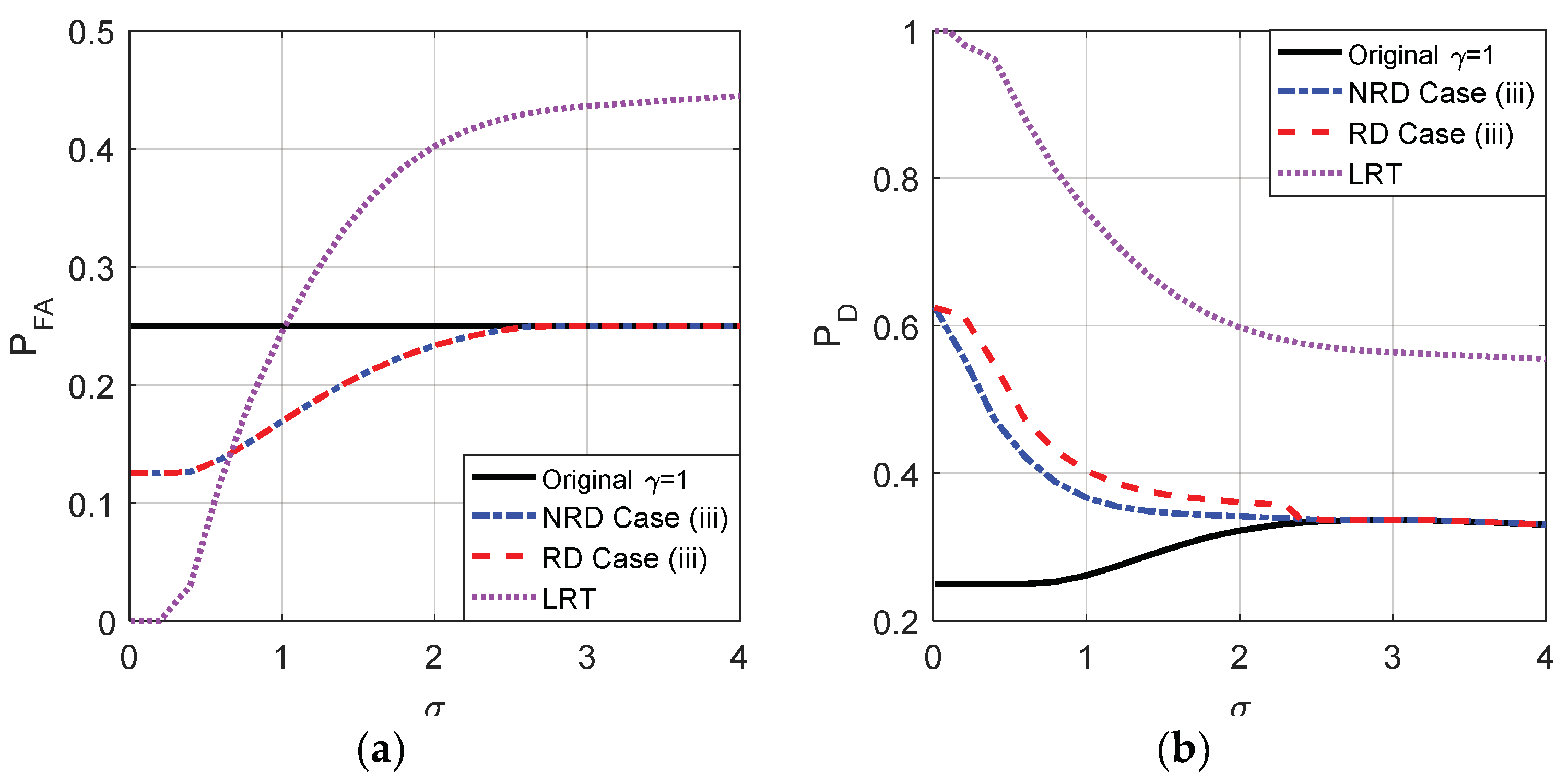
Figure 12 compares the probabilities of false-alarm and detection obtained by the original detector, LRT and case (iii) when randomization can or cannot be allowed where
and the original threshold is
. As shown in
Figure 12, compared to the non-randomization case, the detection probability obtained in case (iii) is further improved for
by allowing randomization of the two thresholds while the false-alarm probability cannot be further decreased. Moreover, the
of LRT increases when
increases and will be greater than that obtained in case (iii) when
and the original detector when
.
Figure 13 illustrates the Bayes risks for the original detector, LRT and noise enhanced decision solutions when the randomization between detectors can or cannot be allowed for different
, where
,
, and
denote case (i), case (ii), and case (iii), respectively. As plotted in
Figure 13, the Bayes risks obtained in case (i), (ii), and (iii) are smaller than the original detector, and the Bayes risk of LRT is the smallest one. Furthermore, the Bayes risk obtained in the randomization case is smaller than that obtained in the non-randomization case.
As shown in
Figure 14, when the original threshold
, under the constraints that
and
, the false-alarm probability can be greatly decreased by allowing randomization between different thresholds compared to the non-randomization case when
. In addition, LRT performs best on
. Accordingly, the minimum false-alarm probability in case (i) is obtained by a suitable randomization of
and
with probabilities
and
, respectively, where
. Through some simple analyses, under the same constraints, the detection probability obtained when there exists randomization between different thresholds cannot be greater than that obtained in the non-randomization case. Thus the maximum detection probability in case (ii) is the same as that illustrated in
Figure 10, which is achieved by choosing a threshold
and adding the corresponding optimal additive noise to the observation.
Case (iii) can also be achieved by the randomization of the noise enhanced solutions for case (i) and case (ii) with the probabilities
and
, respectively. As shown in
Figure 15, compared to the non-randomization case, the false-alarm probability obtained in case (iii) is greatly improved by allowing randomization of the two thresholds while the detection probability cannot be increased when the original threshold
. Although the
of LRT is always superior to that obtained in other cases, the
of LRT will be smaller than that obtained by the original detector and case (iii) when
increases to a certain extent.
Figure 16 illustrates the Bayes risks for the original detector, LRT and the noise enhanced decision solutions for different
. Also,
,
, and
denote case (i), case (ii) and case (iii), respectively. As plotted in
Figure 16, the Bayes risks obtained by the three cases are smaller than the original detector for
. The smallest one of the three is achieved in case (i) if
or case (ii) if
when no randomization exists between the thresholds, while it is achieved in case (i) if
or case (ii) if
when the randomization between the thresholds is allowed. Obviously, the Bayes risk obtained in the randomization case is not greater than that obtained in the non-randomization case. In addition, LRT achieves the minimum Bayes risk when
and the maximum Bayes risk when
.
As analyzed in 5.1, if the structure of a detector does not change with the decision thresholds, the optimal noise enhanced detection performances for different thresholds are the same, which can be achieved by adding the corresponding optimal noise. In such case, no improvement can be obtained by allowing randomization between different decision thresholds. On the other hand, if different thresholds correspond to different structures as shown in (39) and (40), randomization between different decision thresholds can introduce new noise enhanced solutions to improve the detection performance further under certain conditions.


