A Quantal Response Statistical Equilibrium Model of Induced Technical Change in an Interactive Factor Market: Firm-Level Evidence in the EU Economies


Abstract
:1. Introduction
2. Patterns of Technical Change
2.1. Data
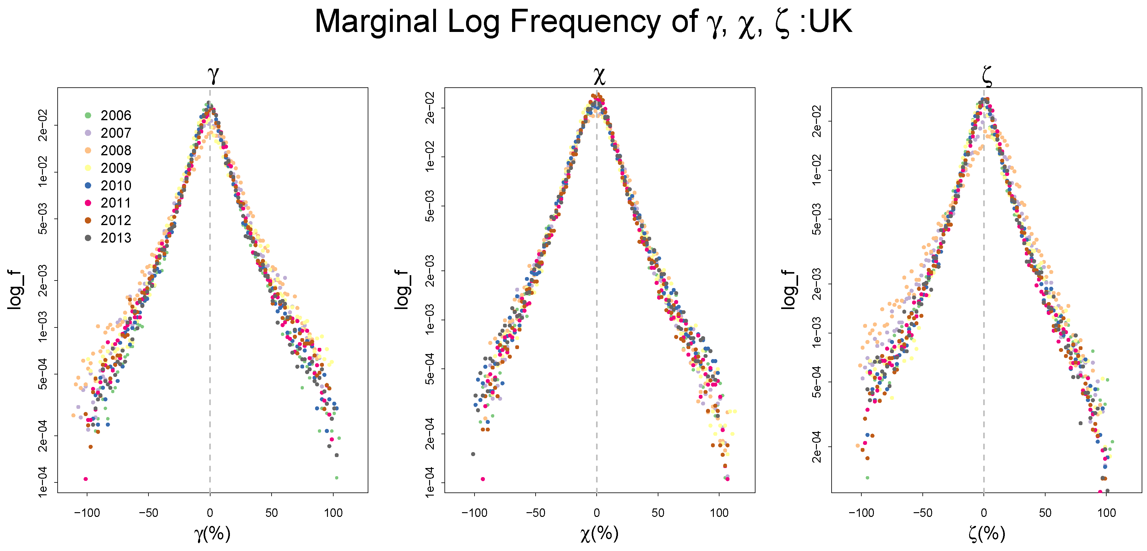
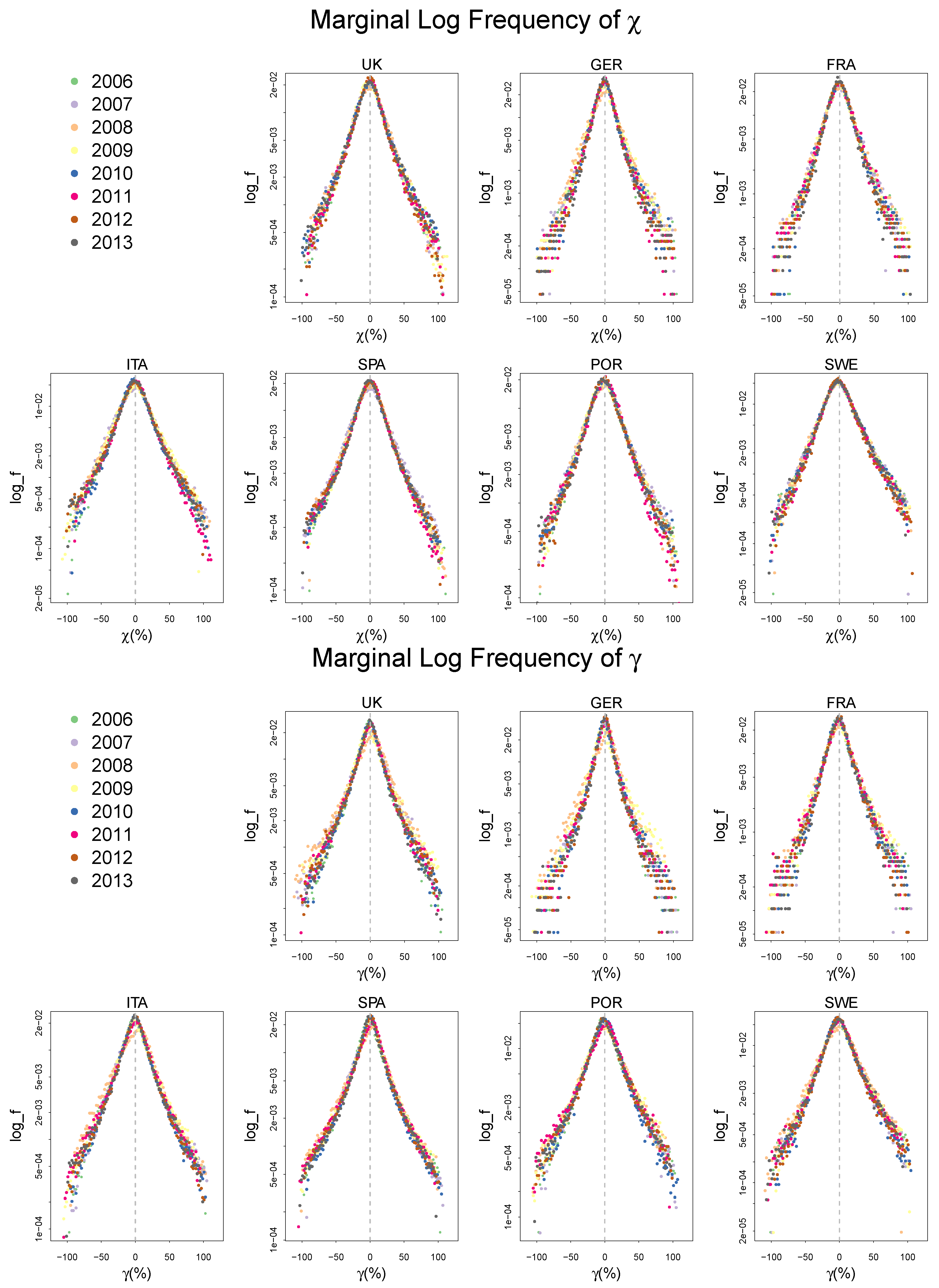
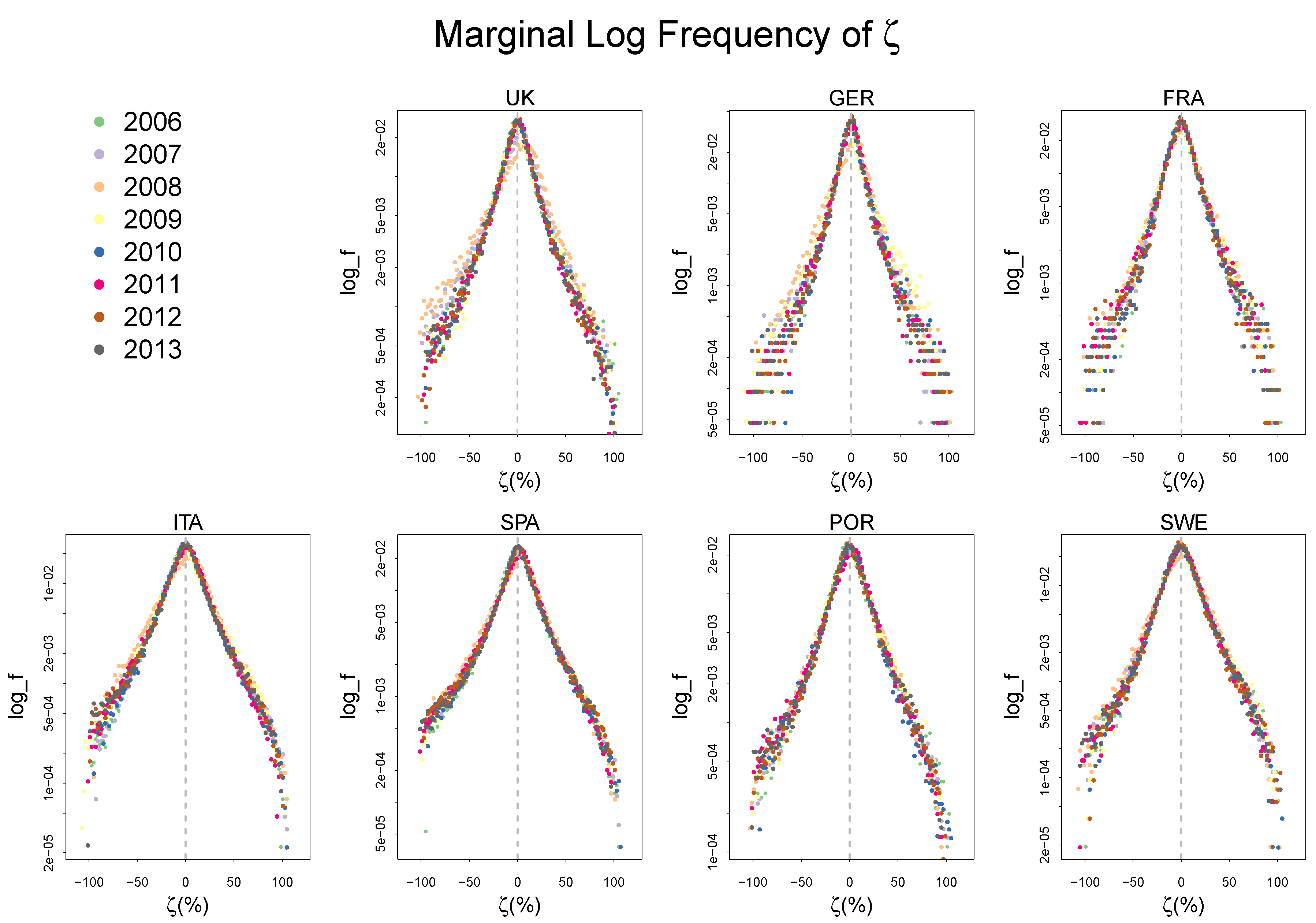
2.2. Empirical Distributions of , and,
3. A Statistical Equilibrium Model of the ITC
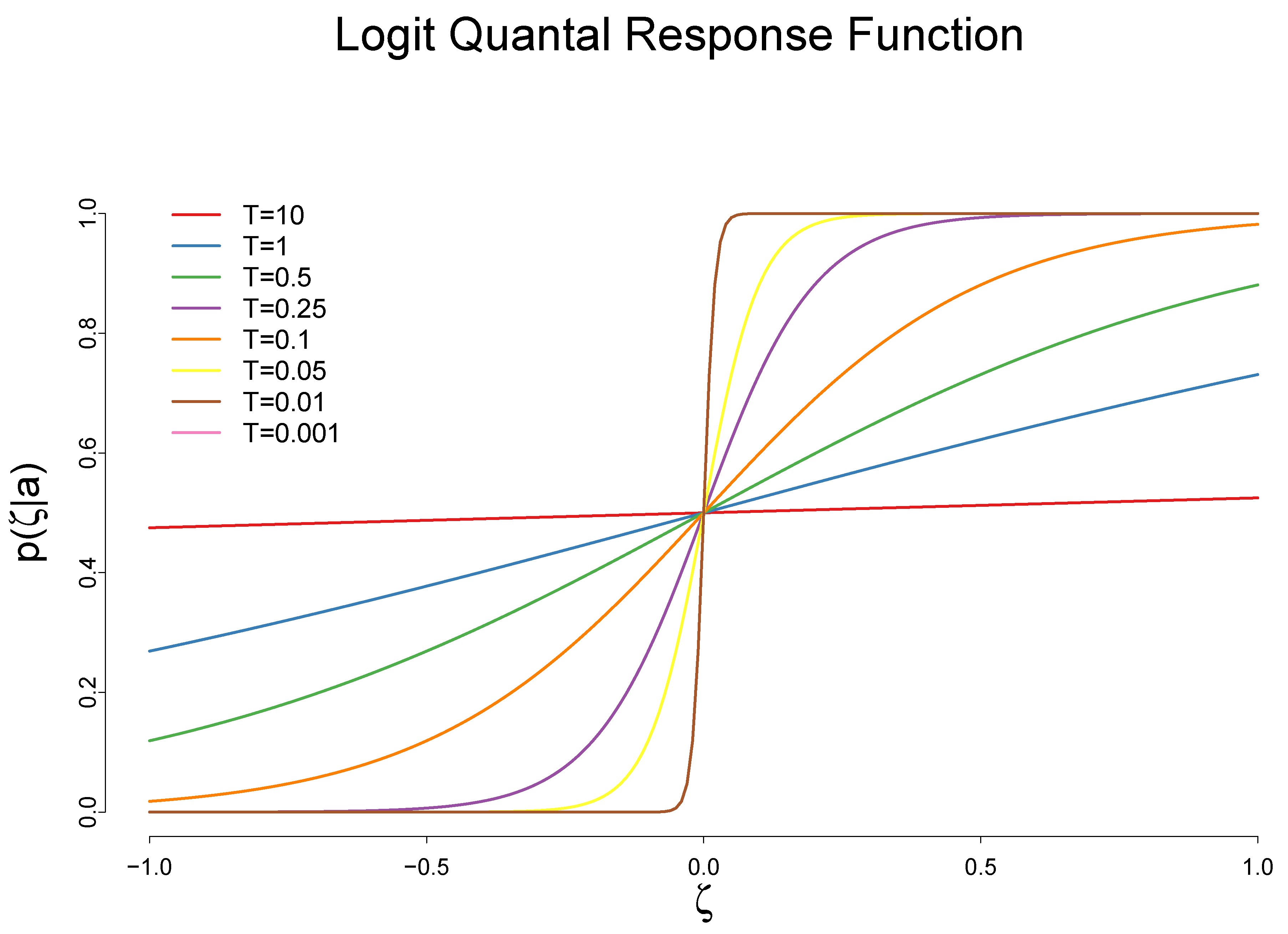
3.1. The Impact of the Cost Reduction on Adoption of a New Technology
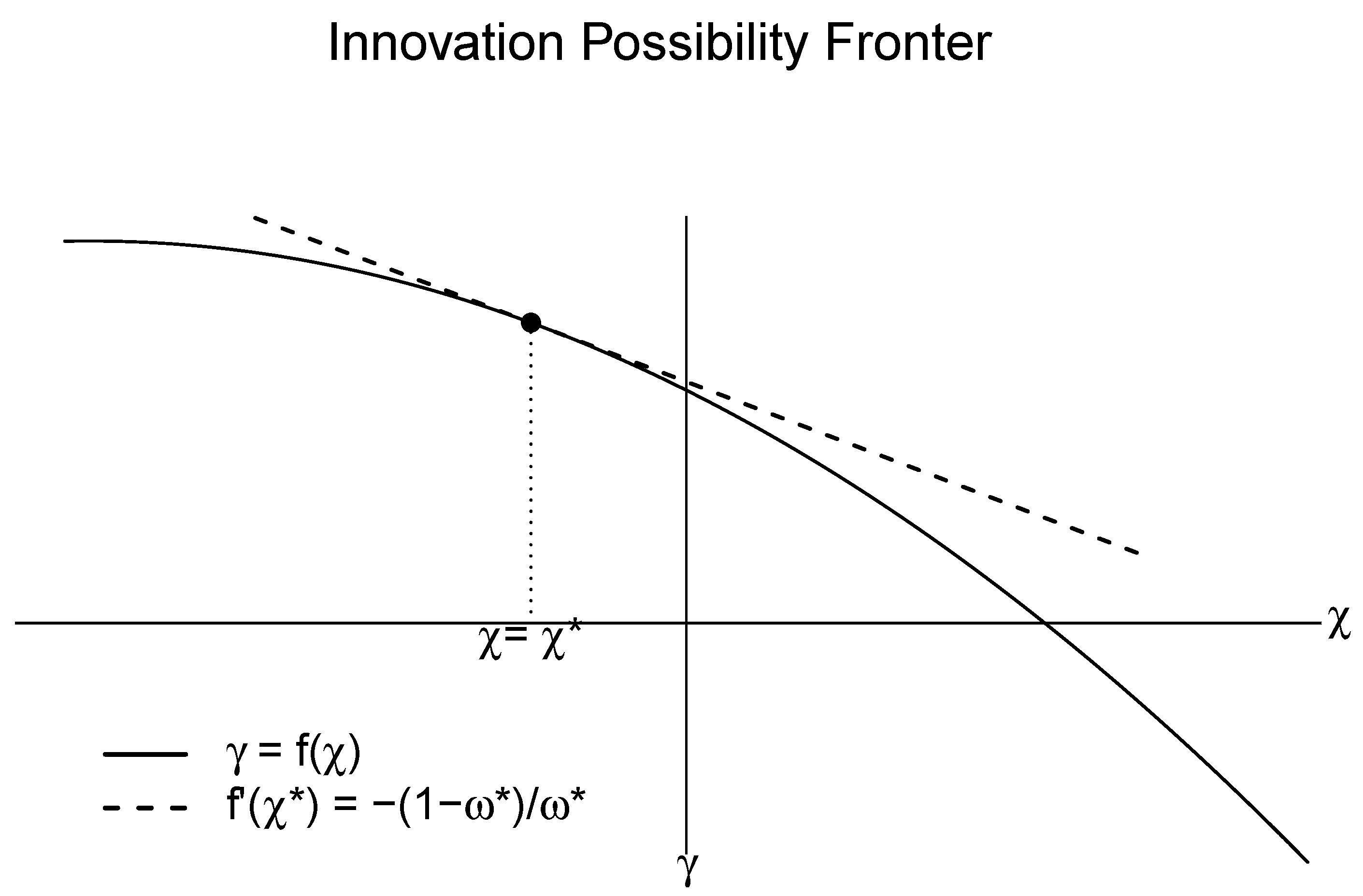
3.2. The Impact of the Adoption of a New Technology on the Rate of Cost Reduction
3.3. Maximum Entropy Program of the Quantal Response ITC Model
4. Bayesian Estimation of the Model
4.1. Model Specification
4.2. Result
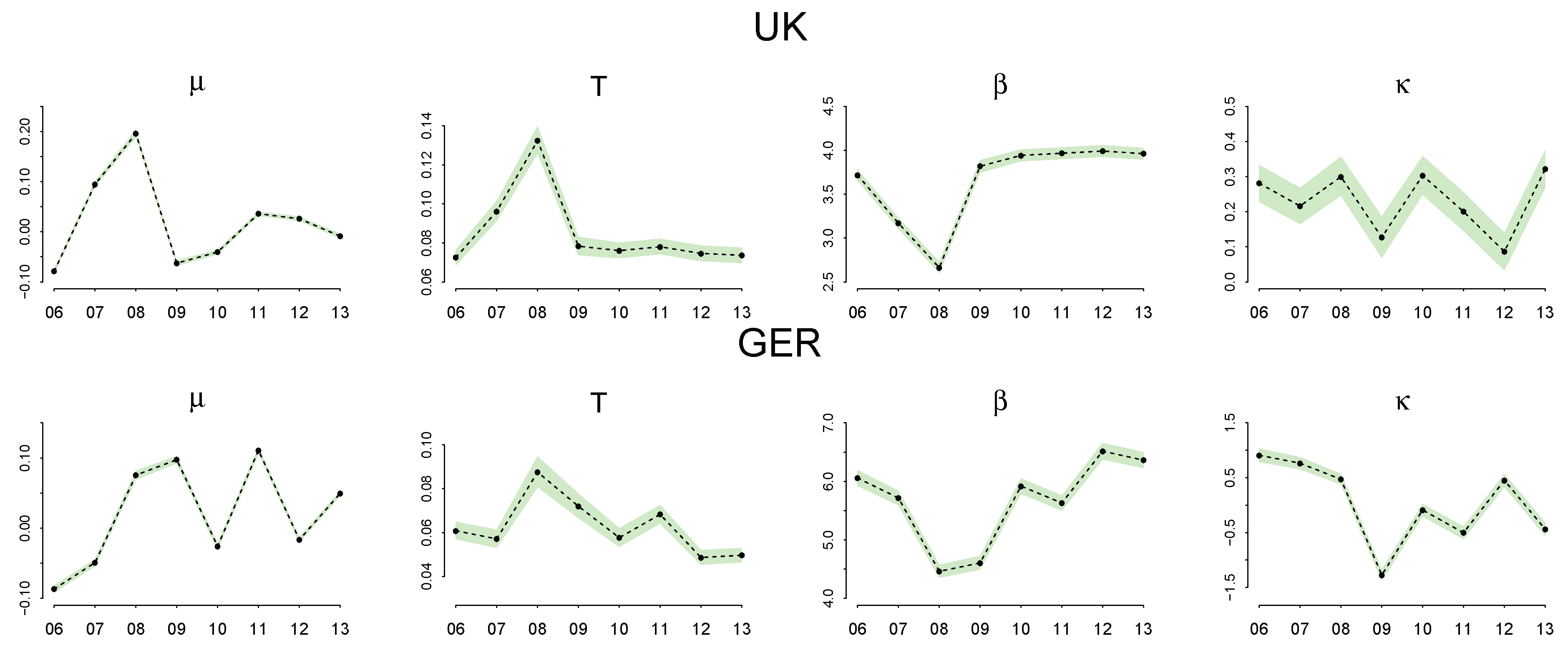
Parameter Estimation
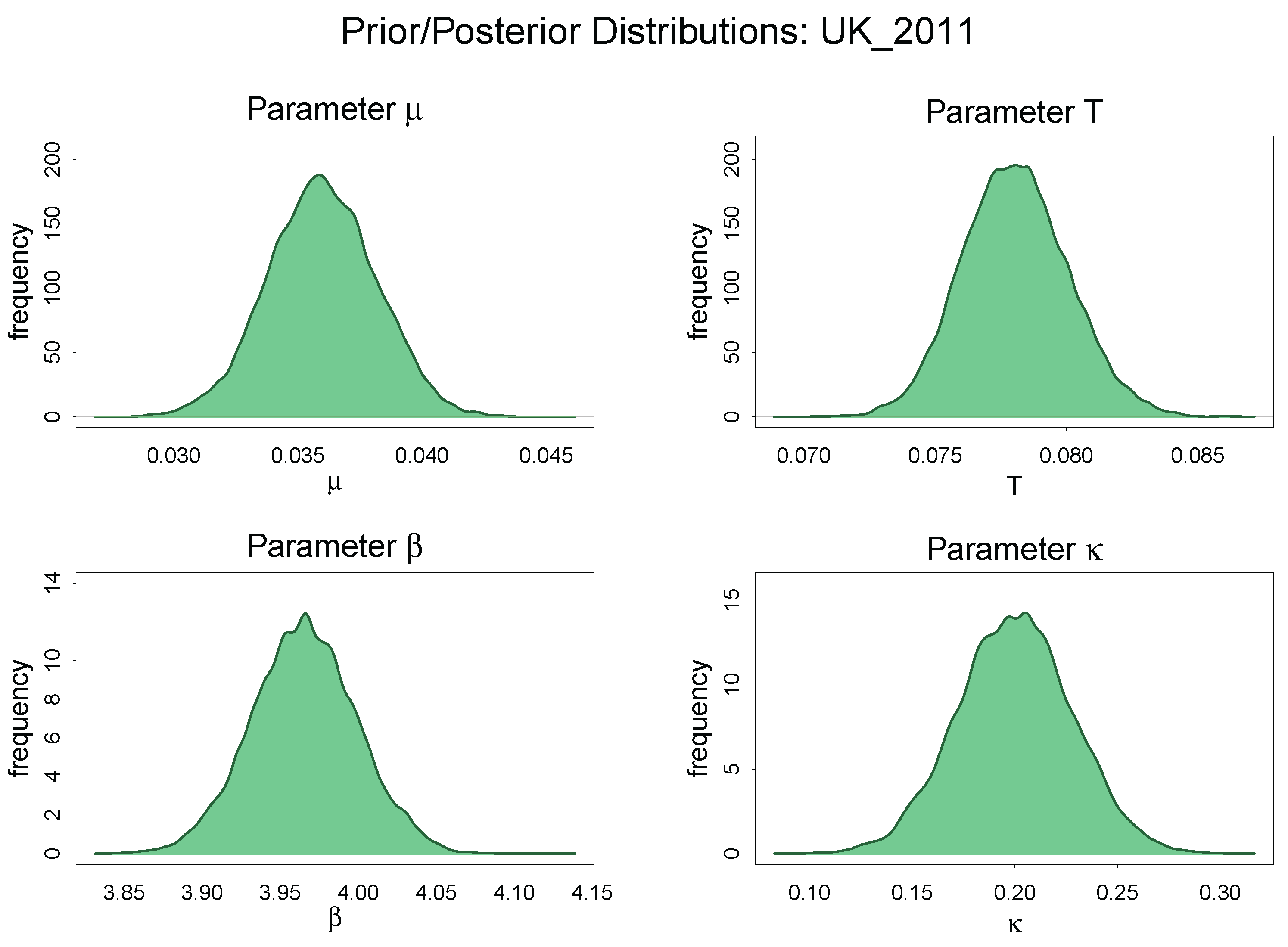
Comparison of Prior and Posterior Distribution: UK 2011
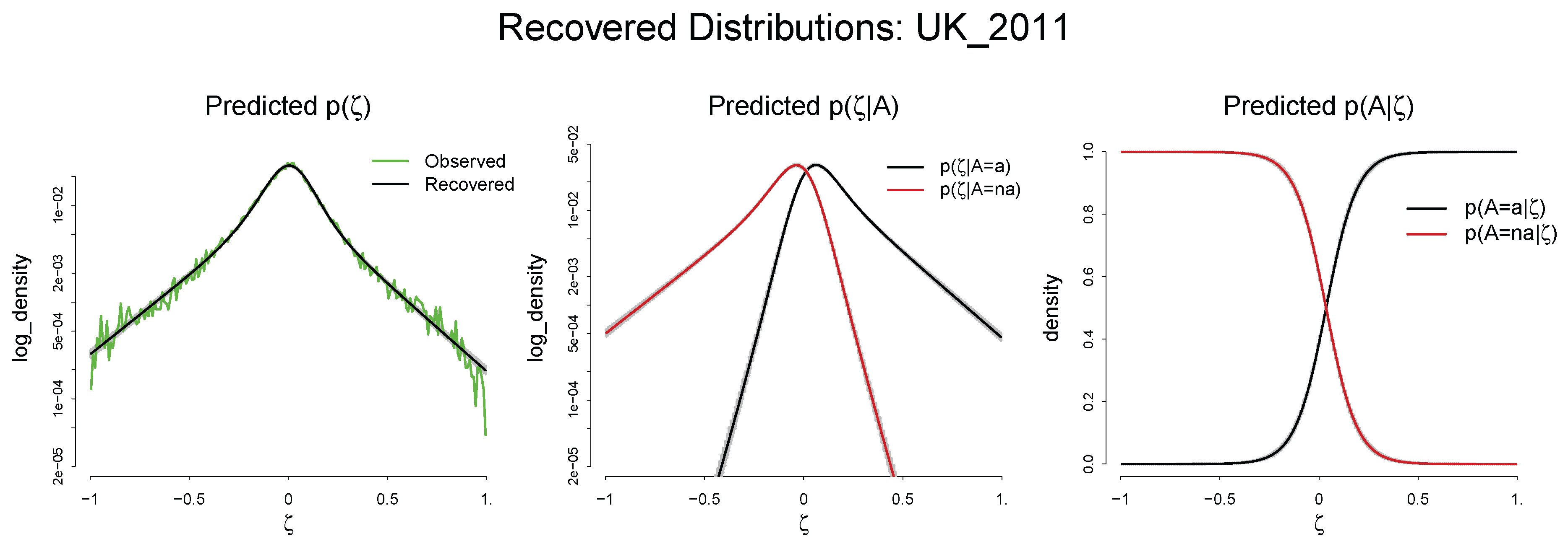
Predicted , , and : UK 2011
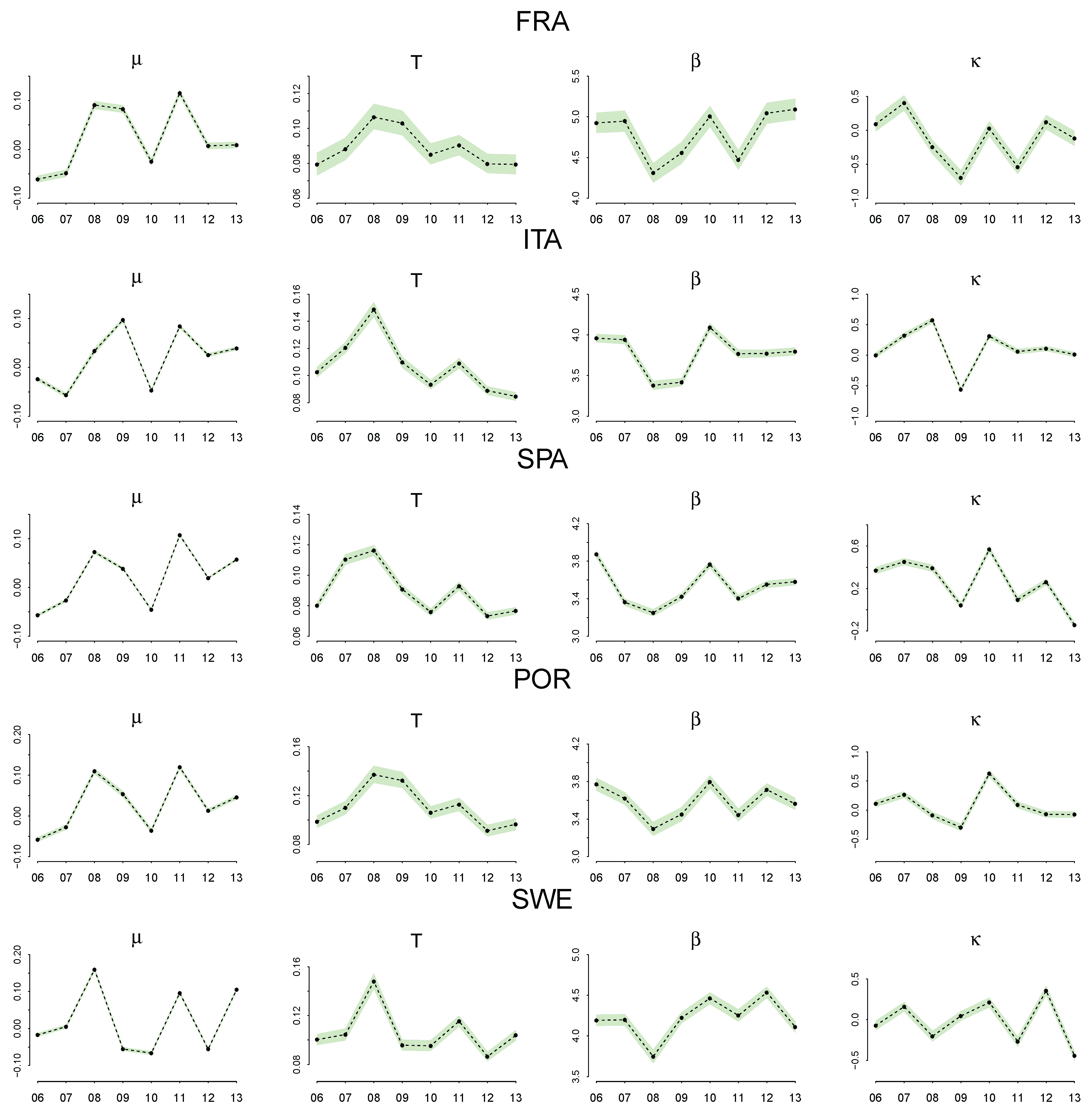
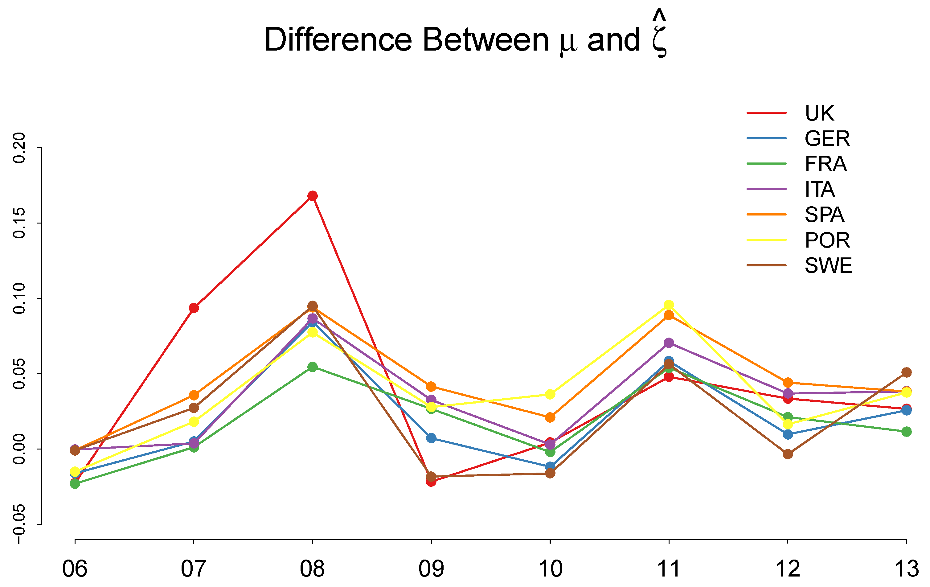
4.3. Discussion of the Estimated Parameters, and
5. Discussion
6. Conclusions
Acknowledgments
Conflicts of Interest
Appendix A. Summary Statistics of the Frequency Distributions of γ, χ, and ζ

| Country | UK | GER | FRA | ITA | SPA | POR | SWE |
|---|---|---|---|---|---|---|---|
| (%) | 0.98 | 0.43 | 1.15 | −0.80 | −1.02 | 0.65 | 1.10 |
| (%) | −6.22 | −1.13 | −1.89 | −3.38 | −6.57 | −4.43 | −2.12 |
| (%) | 7.20 | 1.56 | 3.04 | 2.58 | 5.55 | 5.08 | 3.22 |
| (%) | −2.10 | −0.08 | 0.33 | −1.49 | −2.46 | −0.91 | −0.24 |
Appendix B. Soofi ID Index
| Year | UK | GER | FRA | ITA | SPA | POR | SWE |
|---|---|---|---|---|---|---|---|
| 2006 | 0.006 | 0.069 | 0.043 | 0.006 | 0.010 | 0.010 | 0.006 |
| 2007 | 0.020 | 0.056 | 0.060 | 0.008 | 0.010 | 0.007 | 0.011 |
| 2008 | 0.061 | 0.061 | 0.029 | 0.025 | 0.010 | 0.009 | 0.015 |
| 2009 | 0.007 | 0.050 | 0.039 | 0.020 | 0.003 | 0.012 | 0.008 |
| 2010 | 0.007 | 0.027 | 0.035 | 0.008 | 0.013 | 0.018 | 0.015 |
| 2011 | 0.004 | 0.014 | 0.019 | 0.004 | 0.003 | 0.007 | 0.007 |
| 2012 | 0.008 | 0.017 | 0.018 | 0.003 | 0.002 | 0.009 | 0.004 |
| 2013 | 0.005 | 0.015 | 0.027 | 0.004 | 0.005 | 0.008 | 0.008 |
References
- Jaynes, E.T. Where Do We Stand on Maximum Entropy? In The Maximum Entropy Formalism; Levine, R.D., Tribus, M., Eds.; MIT Press: Cambridge, MA, USA, 1978; pp. 15–118. [Google Scholar]
- Jaynes, E.T. Information theory and statistical mechanics. Phys. Rev. 1957, 106, 620–630. [Google Scholar] [CrossRef]
- Farjoun, E.; Machover, M. Laws of Chaos: Probabilistic Approach to Political Economy; Verso Books: New York, NY, USA, 1983. [Google Scholar]
- Foley, D.K. A Statistical Equilibrium Theory of Market. J. Econ. Theory 1994, 62, 321–345. [Google Scholar] [CrossRef]
- Stutzer, M.J. A Bayesian Approach to Diagnostic of Asset Pricing Models. J. Econ. 1995, 68, 369–397. [Google Scholar] [CrossRef]
- Stutzer, M.J. Simple Entropic Derivation of a Generalized Black-Scholes Option Pricing Model. Entropy 2010, 2, 70–77. [Google Scholar] [CrossRef]
- Sims, C.A. Implications of rational inattention. J. Monetary Econ. 2003, 50, 665–690. [Google Scholar] [CrossRef]
- Smith, E.; Foley, D.K. Classical thermodynamics and economic general equilibrium theory. J. Econ. Dyn. Control 2008, 32, 7–65. [Google Scholar] [CrossRef]
- Toda, A.A. Existence of a statistical equilibrium for an economy with endogenous offer sets. Econ. Theory 2010, 45, 379–415. [Google Scholar] [CrossRef]
- Toda, A.A. Bayesian general equilibrium. Econ. Theory 2015, 58, 375–411. [Google Scholar] [CrossRef]
- Lux, T. Applications of statistical physics in finance and economics. In Handbook on Complexity Research; Rosser, J.B., Ed.; Edward Elgar: Cheltenham, UK, 2009; pp. 213–258. [Google Scholar]
- Zhou, R.; Cai, R.; Tong, G. Applications of Entropy in Finance: A Review. Entropy 2013, 15, 4909–4931. [Google Scholar] [CrossRef]
- Rosser, J.B. Entropy and econophysics. Eur. Phys. J. Spec. Top. 2016, 225, 3091–3104. [Google Scholar] [CrossRef]
- Yang, J. Information theoretic approaches in economics. J. Econ. Surv. 2017. [Google Scholar] [CrossRef]
- Scharfenaker, E.; Foley, D.K. Quantal Response Statistical Equilibrium in Economic Interactions: Theory and Estimation. Entropy 2017, 19, 444. [Google Scholar] [CrossRef]
- Michl, T.; Foley, D.K. Growth and Distribution; Harvard University Press: London, UK, 1999. [Google Scholar]
- Alfarano, S.; Milaković, M. Does Classical Competition Explain the Statistical Features of Firm Growth? Econ. Lett. 2008, 101, 272–274. [Google Scholar] [CrossRef]
- Alfarano, S.; Milaković, M.; Irle, A.; Kauschke, J. A Statistical Equilibrium Model of Competitive Firms. J. Econ. Dyn. Control 2012, 36, 136–149. [Google Scholar] [CrossRef]
- Jaynes, E.T. Probability Theory: The Logic of Science; Cambridge University Press: Cambridge, UK, 2003. [Google Scholar]
- Kapur, J.N. Maximum-Entropy Models in Science and Engineering; John Wiley & Sons: Hoboken, NJ, USA, 1998. [Google Scholar]
- Von Weisäcker, C.C. A New Technical Progress Function (1962). Ger. Econ. Rev. 2010, 11, 248–265. [Google Scholar] [CrossRef]
- Kennedy, C. Induced Bias in Innovation and the Theory of Distribution. Econ. J. 1964, 74, 541–547. [Google Scholar] [CrossRef]
- Samuelson, P.A. A Theory of Induced Innovation along Kennedy-Weisäcker Lines. Rev. Econ. Stat. 1965, 47, 343–356. [Google Scholar] [CrossRef]
- Drandakis, E.M.; Phelps, E.S. A Model of Induced Invention, Growth and Distribution. Econ. J. 1966, 76, 823–840. [Google Scholar] [CrossRef]
- Foley, D. Endogenous Technical Change with Externalities in a Classical Growth model. J. Econ. Behav. Organ. 2003, 52, 167–189. [Google Scholar] [CrossRef]
- McFadden, D.L. Quantal Choice Analaysis: A Survey. Ann. Econ. Soc. Meas. 1976, 5, 363–390. [Google Scholar]
- McFadden, D.L. Economic choices. Am. Econ. Rev. 1976, 91, 351–378. [Google Scholar] [CrossRef]
- Train, K. Discrete Choice Methods with Simulation; Cambridge University Press: Cambridge, UK, 2009. [Google Scholar]
- McKelvey, R.D.; Palfrey, T.R. Quantal Response Equilibria for Normal Form Games. Games Econ. Behav. 1995, 10, 6–38. [Google Scholar] [CrossRef]
- Chen, H.C.; Friedman, J.W.; Thisse, J.F. Boundedly Rational Nash Equilibrium: A Probabilistic Choice Approach. Games Econ. Behav. 1997, 18, 32–54. [Google Scholar] [CrossRef]
- McKelvey, R.D.; Palfrey, T.R. Quantal Response Equilibria for Extensive Form Games. Exp. Econ. 1998, 1, 9–41. [Google Scholar] [CrossRef]
- Wolpert, D. Information Theory—The Bridge Connecting Bounded Rational Game Theory and Statistical Physics. In Complex Engineered Systems; Braha, D., Minai, A., Bar-Yam, Y., Eds.; Springer: Berlin, Heidelberg, 2006; pp. 262–290. [Google Scholar]
- Dos Santos, P.L. The Principle of Social Scaling. Complexity 2017, 2017, 8358909. [Google Scholar] [CrossRef]
- Kullback, S.; Leibler, R. On information and sufficiency. Ann. Math. Stat. 1951, 22, 79–86. [Google Scholar] [CrossRef]
- Gamerman, D.; Lopes, H.F. Markov Chain Monte Carlo: Stochastic Simulation for Bayesian Inference, 2nd ed.; CRC Press: Boca Raton, FL, USA, 2008. [Google Scholar]
- Minh, D.D.L.; Minh, D.L. Understanding the Hastings Algorithm. Commun. Stat. Simul. Comput. 2015, 44, 332–349. [Google Scholar] [CrossRef]
- Gelman, A.; Carlin, J.B.; Stern, H.S.; Dunson, D.B.; Vehtari, A.; Rubin, D.B. Bayesian Data Analysis, 3rd ed.; CRC Press: Boca Raton, FL, USA, 2013. [Google Scholar]
- Golan, A. Information and Entropy Econometrics—Editor’s View. J. Econ. 2002, 107, 1–15. [Google Scholar] [CrossRef]
- Golan, A.; Judge, G.G.; Miller, D. Maximum Entropy Econometrics: Robust Estimation with Limited Data; Wiley: Hoboken, NJ, USA, 1996. [Google Scholar]
- Soofi, E.S.; Ebrahimi, N.; Habibullah, M. Information Distinguishability with Application to Analysis of Failure Data. J. Am. Stat. Assoc. 1995, 90, 657–668. [Google Scholar] [CrossRef]
- Soofi, E.; Retzer, J. Information indices: Unification and applications. J. Econ. 2002, 107, 17–40. [Google Scholar] [CrossRef]


© 2018 by the author. Licensee MDPI, Basel, Switzerland. This article is an open access article distributed under the terms and conditions of the Creative Commons Attribution (CC BY) license (http://creativecommons.org/licenses/by/4.0/).
Share and Cite
Yang, J. A Quantal Response Statistical Equilibrium Model of Induced Technical Change in an Interactive Factor Market: Firm-Level Evidence in the EU Economies. Entropy 2018, 20, 156. https://doi.org/10.3390/e20030156
Yang J. A Quantal Response Statistical Equilibrium Model of Induced Technical Change in an Interactive Factor Market: Firm-Level Evidence in the EU Economies. Entropy. 2018; 20(3):156. https://doi.org/10.3390/e20030156
Chicago/Turabian StyleYang, Jangho. 2018. "A Quantal Response Statistical Equilibrium Model of Induced Technical Change in an Interactive Factor Market: Firm-Level Evidence in the EU Economies" Entropy 20, no. 3: 156. https://doi.org/10.3390/e20030156
APA StyleYang, J. (2018). A Quantal Response Statistical Equilibrium Model of Induced Technical Change in an Interactive Factor Market: Firm-Level Evidence in the EU Economies. Entropy, 20(3), 156. https://doi.org/10.3390/e20030156