Function Analysis of the Euclidean Distance between Probability Distributions

Abstract

Minimization of the Euclidean distance between output distribution and Dirac delta functions as a performance criterion is known to match the distribution of system output with delta functions. In the analysis of the algorithm developed based on that criterion and recursive gradient estimation, it is revealed in this paper that the minimization process of the cost function has two gradients with different functions; one that forces spreading of output samples and the other one that compels output samples to move close to symbol points. For investigation the two functions, each gradient is controlled separately through individual normalization of each gradient with their related input. From the analysis and experimental results, it is verified that one gradient is associated with the role of accelerating initial convergence speed by spreading output samples and the other gradient is related with lowering the minimum mean squared error (MSE) by pulling error samples close together.

1. Introduction

Adaptive signal processing is carried out by minimizing or maximizing an appropriate performance criterion for adjusting weights of algorithms designed based on that criterion [1]. The mean squared error (MSE) criterion that measures the average of the squares of the error signal is widely employed in the Gaussian noise environment. However in non-Gaussian noise like impulsive noise, the averaging process of squared error samples that may mitigate the effects of the Gaussian noise is defeated because a single large, impulse can dominate these sums. As recent signal processing methods, the information-theoretic learning (ITL) is based on the information potential concept that data samples can be treated as physical particles in an information potential field where they interact with each other by information forces [2]. The ITL method usually exploits probability distribution functions constructed by the kernel density estimation method with the Gaussian kernel.

Among the ITL criteria, Euclidian distance (ED) between two distributions has been known to be effective in signal processing fields demanding similarity measure functions [3,4,5]. For training of adaptive systems for medical diagnosis, the ED criterion has been successfully applied to distinguish biomedical datasets [6]. For finite impulse response (FIR) adaptive filter structures in impulsive noise environments, ED between the output distribution and a set of Dirac delta functions has been used as an efficient performance criterion taking advantage of the outlier-cutting effect of Gaussian kernel for output pairs and symbol-output pairs [7]. In this approach with output distribution and delta functions, minimization of the ED (MED) leads to adaptive algorithms that adjust weights so as for the output distribution to be formed into the shape of delta functions located at each symbol point, that is, output samples concentrate on symbol points. Though the blind MED algorithm shows superior performance of robustness against impulsive noise and channel distortions, a drawback of heavy computational burden lies in it. The computational complexity is due in large part to the double summation operations at each iteration time for its gradient estimation. A follow-up study [8], however, shows that the drawback can be reduced significantly by employing a recursive gradient estimation method.

The gradient in ED minimization process of the MED algorithm has two components; one for kernel function of output pairs and the other for kernel function of symbol-output pairs. The roles of these two components have not been investigated or analyzed in scientific literature. In this paper, we analyze the roles of the two components and prove the analysis through controlling each component individually by normalizing each component with component-related input power. Through simulation in multipath channel equalization under impulsive noise, their roles of managing sample pairs are verified, and it is shown that the proposed method of controlling each component through power normalization increases convergence speed and lowers steady state MSE significantly in multipath and impulsive noise environment.

2. MSE Criterion and Related Algorithms

Employing the tapped delay line (TDL) structure, the output y_k becomes $y_k=W_k^T{X}_k$ at time k with the input vector $X_k={\left[x_k,x_{k-1},\dots ,x_{k-L+1}\right]}^T$ and weight $W_k={\left[w_{0.k},w_{1,k},\dots ,w_{L-1,k}\right]}^T$. Given the desired signal d_k chosen randomly among the M symbol points (A₁, A₂, …, A_M), the system error is calculated as e_k = d_k − y_k. In blind equalization, the constant modulus error $e_{\mathrm{CME},k}={\left|y_k\right|}^2-R_2$ where $R_2=E[{\left|d_k\right|}^4]/E[{\left|d_k\right|}^2]$ is mostly used [9].

The MSE criterion, one of the most widely used criteria, is the statistical average E[·] of error power $e_k^2$ in supervised equalization and of CME power ${({\left|y_k\right|}^2-R_2)}^2$ in a blind one. For practical implementation we can use the instant squared error $e_k^2$ as a cost function in supervised equalization. With the gradient $\frac{\partial e_k^2}{W}=-2e_k{X}_k$ and a step size μ_LMS, minimization of $e_k^2$ leads to the least mean square (LMS) algorithm [1]:

$$W_{k+1}=W_k-{\mu }_{\mathrm{LMS}}\frac{\partial e_k^2}{\partial W}=W_k+{\mu }_{\mathrm{LMS}}2e_k{X}_k$$

(1)

As an extension of the LMS algorithm, the normalized LMS (NLMS) algorithm has been introduced where the gradient is normalized as proportional to the inverse of the dot product of the input vector with itself ${\Vert X_k\Vert }^2=X_k^T{X}_k={{\displaystyle \sum }}_{m=0}^{L-1}{x}_{k-m}^2$ as a result of minimizing weight perturbation ${\Vert W_{k+1}-W_k\Vert }^2$ of the LMS algorithm [1]. Then the NLMS algorithm becomes:

$$W_{k+1}=W_k+{\mu }_{\mathrm{NLMS}}\frac{e_k{X}_k}{{\displaystyle \sum _{m=0}^{L-1}{x}_{k-m}^2}}$$

(2)

The NLMS algorithm is known to be more stable with unknown signals and effective in real time adaptive systems [10,11]. We can see under impulsive noise environments that a single large error sample induced by impulsive noise can generate large weight perturbations. The perturbation becomes zero only when the error e_k is zero. So we can predict that the weight update process (1) may be unstable so that it requires a very small step size in impulsive noise environment. Also the LMS and NLMS algorithms utilizing instant error power $e_k^2$ may cause instability in an impulsive noise environment.

3. ED Criterion and Entropy

Unlike the MSE based on error power, probability distribution functions can be used in constructing performance criterion. As one of the criteria utilizing distributions, the ED between the distribution of transmitted symbol f_D(d) and the equalizer output distribution f_Y(y) is defined as (3) [3,6].

$$\mathrm{ED}={\displaystyle \int {[f_D^{}(\alpha )-f_Y^{}(\alpha )]}^2\mathrm{d}\alpha }$$

(3)

Assuming that modulation schemes are known to receivers beforehand and all the M symbol points (A₁, A₂, …, A_M) are equally likely, the distribution of the transmitted symbols can be expressed as:

$$f_D(\alpha )=\frac{1}{M}[\delta (\alpha -A_1)+\delta (\alpha -A_2)+\dots +\delta (\alpha -A_m)+\dots +\delta (\alpha -A_M)]$$

(4)

The output distribution can be estimated based on kernel density estimation method $f_Y\left(y\right)=1/N{{\displaystyle \sum }}_{i=1}^N{G}_{\sigma }\left(y-y_i\right)$ with a set of available N output samples {y₁, y₂, …, y_N} [6].

Then the ED can be expressed as:

$$\mathrm{ED}=\frac{1}{M}+\frac{1}{N^2}{\displaystyle \sum _{i=1}^N{\displaystyle \sum _{j=1}^N{G}_{\sigma \sqrt{2}}(y_j-y_i)}}-2\frac{1}{M}\frac{1}{N}{\displaystyle \sum _{m=1}^M{\displaystyle \sum _{i=1}^N{G}_{\sigma }(A_m-y_i)}}$$

(5)

The first term 1/M in (5) is a constant which is not adjustable, so the ED can be reduced to the following performance criterion C_ED [7]:

$$C_{\mathrm{ED}}=\frac{1}{N^2}{\displaystyle \sum _{i=1}^N{\displaystyle \sum _{j=1}^N{G}_{\sigma \sqrt{2}}(y_j-y_i)}}-2\frac{1}{M}\frac{1}{N}{\displaystyle \sum _{m=1}^M{\displaystyle \sum _{i=1}^N{G}_{\sigma }(A_m-y_i)}}$$

(6)

In ITL methods, data samples are treated as physical particles interacting with each other. If we place physical particles in the locations of y_i and y_j, the Gaussian kernel $G_{\sigma \sqrt{2}}\left(y_j-y_i\right)$ produces an exponentially decaying positive value as the distance between the two particles increases. This leads us consider the Gaussian kernel $G_{\sigma \sqrt{2}}\left(y_j-y_i\right)$ as a potential field-inducing interaction among particles. Then ${{\displaystyle \sum }}_{j=1}^N{G}_{\sigma \sqrt{2}}\left(y_j-y_i\right)$ corresponds to the sum of interactions on the i-th particle and $1/N^2{{\displaystyle \sum }}_{i=1}^N{{\displaystyle \sum }}_{j=1}^N{G}_{\sigma \sqrt{2}}\left(y_j-y_i\right)$ is the averaged sum of all pairs of interactions. This summed potential energy is referred to as information potential in ITL methods [2]. Therefore, the term $\frac{1}{M}\frac{1}{N}{{\displaystyle \sum }}_{m=1}^M{{\displaystyle \sum }}_{i=1}^N{G}_{\sigma }\left(A_m-y_i\right)$ in (6) is the information potential between symbol points and output samples, and $1/N^2{{\displaystyle \sum }}_{i=1}^N{{\displaystyle \sum }}_{j=1}^N{G}_{\sigma \sqrt{2}}\left(y_j-y_i\right)$ in (6) indicates the information potential among output samples themselves.

On the other hand, the information potential can be interpreted in the concept of entropy that can be described in terms of “energy dispersal” or the “spreading of energy” [11]. As one of the convenient entropy definitions, Reny’s entropy of order 2, H_Reny(y) is defined in (7) as logarithm of the sum of the power of probability which is much easier to estimate [2]:

$$H_{\mathrm{Reny}}(y)=-\log ({\displaystyle \sum _{i=1}^N{p}_i^2})$$

(7)

When the Reny’s entropy is used along with the kernel density estimation method $f_Y\left(y\right)=1/N{{\displaystyle \sum }}_{i=1}^N{G}_{\sigma }\left(y-y_i\right)$, we obtain a much simpler form of Reny’s quadratic entropy as:

$$H_{\mathrm{Reny}}(y)=-\log (\frac{1}{N^2}{\displaystyle \sum _{i=1}^N{\displaystyle \sum _{j=1}^N{G}_{\sigma \sqrt{2}}(y_j-y_i)}})$$

(8)

This leads to:

$$\frac{1}{N^2}{\displaystyle \sum _{i=1}^N{\displaystyle \sum _{j=1}^N{G}_{\sigma \sqrt{2}}(y_j-y_i)}}=\frac{1}{2^{H_{\mathrm{Reny}}(y)}}$$

(9)

Likewise:

$$\frac{1}{M}\frac{1}{N}{\displaystyle \sum _{m=1}^M{\displaystyle \sum _{i=1}^N{G}_{\sigma }(A_m-y_i)}}=\frac{N}{M}\frac{1}{2^{H_{\mathrm{Reny}}(Am,x)}}$$

(10)

Therefore the cost function C_ED becomes:

$$C_{\mathrm{ED}}=\frac{1}{2^{H_{\mathrm{Reny}}(y)}}-2\frac{N}{M}\frac{1}{2^{H_{\mathrm{Reny}}(Am,x)}}$$

(11)

Equations (9) and (11) indicate that the entropy of output samples increases as the distance (y_j − y_i) between the two information particles y_j and y_i increases. Therefore, (y_j − y_i) can be referred to as entropy-governing output and we can notice that (9) controls the spreading of output samples. Likewise, the term $2\frac{1}{M}\frac{1}{N}{{\displaystyle \sum }}_{m=1}^M{{\displaystyle \sum }}_{i=1}^N{G}_{\sigma }\left(A_m-y_i\right)$ in (6), that is, $2\frac{N}{M}\frac{1}{2^{H_{Reny}\left(A_m,x\right)}}$ in (11) governs dispreading or recombining the sample pairs of symbol points and output samples.

4. Entropy-Governing Variables and Recursive Algorithms

When defining y_j,i = (y_j − y_i) and e_m,i = (A_m – y_i) and X_j.i = (X_j – X_i) for convenience’s sake, y_j,i, e_m,i and X_j,i can be referred to as entropy-governing output, entropy-governing error and entropy-governing input, respectively. Using these entropy-governing variables and the on-line density estimation method $f_{X.k}\left(y\right)=\frac{1}{N}{{\displaystyle \sum }}_{i=k-N+1}^k{G}_{\sigma }\left(y-y_i\right)$ instead of f_Y(y), the cost function at time k, C_ED,k can be written as:

$$C_{\mathrm{ED},k}=U_k-V_k$$

(12)

where:

$$U_k=\frac{1}{2^{H_{\mathrm{Reny}}(y)}}=\frac{1}{N^2}{\displaystyle \sum _{i=k-N+1}^k{\displaystyle \sum _{j=k-N+1}^k{G}_{\sigma \sqrt{2}}(y_{j,i})}}$$

(13)

$$V_k=2\frac{N}{M}\frac{1}{2^{H_{Reny}(Am,x)}}=2\frac{1}{M}\frac{1}{N}{\displaystyle \sum _{i=k-N+1}^k{\displaystyle \sum _{j=k-N+1}^k{G}_{\sigma }(e_{m,}{}_i)}}$$

(14)

Minimization of C_ED,k indicates that U_k forces spreading of output samples and −V_k compels output samples to move close to symbol points. Considering that initial-stage output samples which may have clustered about wrong places due to channel distortion, U_k is associated with the role of getting the output samples to move out in search of each destination, that is, accelerating initial convergence speed. On the other hand, V_k is related with compelling output samples near a symbol point to come close lowering the minimum MSE.

On the other hand, the double summation operations for U_k and V_k impose a heavy computational burden. In the work [8] it has been revealed that each component U_k+1 and V_k+1 of C_ED,k+1 = U_k+1 − V_k+1 can be recursively calculated so that the computational complexity of (12) is significantly reduced as in the following equations (15) and (16):

$$\begin{gathered} U_{k+1}^{}=U_k^{}+\frac{2}{N^2}{\displaystyle \sum _{j=k-N+1}^k{G}_{\sigma \sqrt{2}}(y_{i,k+1})}-\frac{2}{N^2}{\displaystyle \sum _{j=k-N+1}^k\frac{1}{2\sigma \sqrt{\pi }}\exp [\frac{-{(y_{i,k-N+1})}^2}{4{\sigma }^2}]} \\ -\frac{2}{N^2}\frac{1}{2\sigma \sqrt{\pi }}\exp [\frac{-{(y_{k+1,k-N+1})}^2}{4{\sigma }^2}]+\frac{2}{N^2}\frac{1}{2\sigma \sqrt{\pi }} \end{gathered}$$

(15)

Similarly, V_k+1 can be divided into the terms with y_k+1 and the terms with y_k−N+1:

$$V_{k+1}^{}=V_k^{}+\frac{2}{NM}{\displaystyle \sum _{m=1}^M[\frac{1}{\sigma \sqrt{2\pi }}\exp [\frac{-{(e_{m,k+1})}^2}{2{\sigma }^2}]}-\frac{1}{\sigma \sqrt{2\pi }}\exp [\frac{-{(e_{m,k-N+1})}^2}{2{\sigma }^2}]]$$

(16)

The gradients $\raisebox{1ex}{$\partial U_k$}\!\left/ \!\raisebox{-1ex}{$\partial W$}\right.$ and $\raisebox{1ex}{$\partial V_k$}\!\left/ \!\raisebox{-1ex}{$\partial W$}\right.$ are calculated recursively by using Equations (15) and (16) as:

$$\begin{array}{l}\frac{\partial U_k^{}}{\partial W}=\frac{\partial U_{k-1}^{}}{\partial W}+\frac{1}{N^2{\sigma }^2}{\displaystyle \sum _{j=k-N}^{k-1}(y_{k,i})}·\frac{1}{2\sigma \sqrt{\pi }}\exp [\frac{-{(y_{k,i})}^2}{4{\sigma }^2}]·X_{i,k}\\ -\frac{1}{N^2{\sigma }^2}{\displaystyle \sum _{j=k-N}^{k-1}(y_{k-N,i})}·\frac{1}{2\sigma \sqrt{\pi }}\exp [\frac{-{(y_{k-N,i})}^2}{4{\sigma }^2}]·X_{i,k-N}\\ -\frac{1}{N^2{\sigma }^2}(y_{k-N,k})·\frac{1}{2\sigma \sqrt{\pi }}\exp [\frac{-{(y_{k-N,k})}^2}{4{\sigma }^2}]·X_{k,k-N}\end{array}$$

(17)

Similarly, $\raisebox{1ex}{$\partial V_k$}\!\left/ \!\raisebox{-1ex}{$\partial W$}\right.$ is calculated recursively as described below:

$$\begin{array}{l}\frac{\partial V_k^{}}{\partial W}=\frac{\partial V_{k-1}^{}}{\partial W}+\frac{2}{NM{\sigma }^2}{\displaystyle \sum _{m=1}^M[(e_{m,k})·\frac{1}{\sigma \sqrt{2\pi }}\exp [\frac{-{(e_{m,k})}^2}{2{\sigma }^2}]·X_k}\\ -(e_{m,k-N})·\frac{1}{\sigma \sqrt{2\pi }}\exp [\frac{-{(e_{m,k-N})}^2}{2{\sigma }^2}]·X_{k-N}]\end{array}$$

(18)

Since the argument $y_{k,i}\frac{1}{2\sigma \sqrt{\pi }}\exp \left[\frac{{\left(y_{k,i}\right)}^2}{4{\sigma }^2}\right]$ in (17) is a function of the entropy-governing output y_k,i, we can define $y_{k,i}\frac{1}{2\sigma \sqrt{\pi }}\exp \left[\frac{{\left(y_{k,i}\right)}^2}{4{\sigma }^2}\right]$ as the modified entropy-output ${\widehat{y}}_{k,i}$, which becomes a significantly mitigated value through the Gaussian kernel when the entropy-governing output y_k,i is a large value.

$$\stackrel{\wedge }{y_{k,i}}=y_{k,i}\frac{1}{2\sigma \sqrt{\pi }}\exp [\frac{-{(y_{k,i})}^2}{4{\sigma }^2}]$$

(19)

Then (17) becomes

$$\frac{\partial U_k^{}}{\partial W}=\frac{\partial U_{k-1}^{}}{\partial W}+\frac{1}{N^2{\sigma }^2}{\displaystyle \sum _{j=k-N}^{k-1}\stackrel{\wedge }{y_{k,i}}·X_{i,k}}-\frac{1}{N^2{\sigma }^2}{\displaystyle \sum _{j=k-N}^{k-1}\stackrel{\wedge }{y_{k-N,i}}·X_{i,k-N}}-\frac{1}{N^2{\sigma }^2}\stackrel{\wedge }{y_{k-N,k}}·X_{k,k-N}$$

(20)

Similarly, we see that the argument $e_{m,k}\frac{1}{\sigma \sqrt{2\pi }}\exp \left[\frac{-{\left(e_{m,k}\right)}^2}{2{\sigma }^2}\right]$ in (18) is a function of entropy-governing error e_m,k, so that we have the modified entropy-error ${\widehat{e}}_{m,k}$ as:

$$\stackrel{\wedge }{e_{m,k}}=e_{m,k}·\frac{1}{\sigma \sqrt{2\pi }}\exp [\frac{-{(e_{m,k})}^2}{2{\sigma }^2}]$$

(21)

The modified entropy-error ${\widehat{e}}_{m,k}$ also becomes a significantly reduced value through the Gaussian kernel when the entropy-governing error e_m,k is large. Then (18) becomes:

$$\frac{\partial V_k^{}}{\partial W}=\frac{\partial V_{k-1}^{}}{\partial W}+\frac{2}{NM{\sigma }^2}{\displaystyle \sum _{m=1}^M[\stackrel{\wedge }{e_{m,k}}·X_k}-\stackrel{\wedge }{e_{m,k-N}}·X_{k-N}]$$

(22)

Through minimization of C_ED,k = U_k − V_k with the gradients $\raisebox{1ex}{$\partial U_k$}\!\left/ \!\raisebox{-1ex}{$\partial W$}\right.$ and $\raisebox{1ex}{$\partial V_k$}\!\left/ \!\raisebox{-1ex}{$\partial W$}\right.$ obtained by (20) and (22), the following recursive MED (RMED) algorithm can be derived [7]:

$$W_{k+1}=W_k-{\mu }_{\mathrm{RMED}}\frac{\partial (U_k-V_k)}{\partial W}=W_k-{\mu }_{\mathrm{RMED}}(\frac{\partial U_k}{\partial W}-\frac{\partial V_k}{\partial W})$$

(23)

Comparing the gradients of RMED to the gradient $\raisebox{1ex}{$\partial e_k^2$}\!\left/ \!\raisebox{-1ex}{$\partial W$}\right.=-2e_k{X}_k$ of the LMS algorithm in (1) which is composed of error and input, we may find that the gradients $\raisebox{1ex}{$\partial U_k$}\!\left/ \!\raisebox{-1ex}{$\partial W$}\right.$ and $\raisebox{1ex}{$\partial V_k$}\!\left/ \!\raisebox{-1ex}{$\partial W$}\right.$ in (20) and (22) have similar terms ${\widehat{y}}_{k,i}·X_{i,k}$ (modified entropy-output multiplied by entropy-input) and ${\widehat{e}}_{m,k}·X_k$ (modified entropy-error multiplied by input), respectively. Considering that impulsive noise may induce large entropy-governing output y_k,i or entropy-governing error e_m,k, modified entropy-output ${\widehat{y}}_{k,i}$ and modified entropy-error ${\widehat{e}}_{m,k}$ which are significantly mitigated by the Gaussian kernel can be viewed as playing a crucial role in obtaining stable gradients under strong impulsive noise. Therefore we can anticipate that the RMED algorithm (23) can have a low weight perturbation in impulsive noise environments.

5. Input Power Estimation for Normalized Gradient

For the purpose of minimizing the weight perturbation ${\Vert W_{k+1}-W_k\Vert }^2$ of the LMS algorithm in (1), the NLMS algorithm has been introduced where the gradient is normalized by the averaged power of the current input samples ${\Vert X_k\Vert }^2=X_k^T{X}_k={{\displaystyle \sum }}_{m=0}^{L-1}{x}_{k-m}^2$ [1].

$$W_{k+1}=W_k+{\mu }_{\mathrm{NLMS}}\frac{e_k{X}_k}{{\Vert X_k\Vert }^2}$$

(24)

Applying this approach to RMED we propose in this section to normalize the gradients in some ways. Since the role of U_k (spreading output samples) is different from that of V_k (moving output samples close to symbol points), the gradients of (23) can be normalized separately as:

$$W_{k+1}=W_k-{\mu }_{\mathrm{RMED}}\frac{\partial U_k}{\partial W}\frac{1}{P_U(k)}+{\mu }_{\mathrm{RMED}}\frac{\partial V_k}{\partial W}\frac{1}{P_V(k)}$$

(25)

where P_U(k) is the average power of X_i,k and P_V(k) is the average power of X_k as:

$$P_U(k)=\frac{1}{N}{\displaystyle \sum _{i=k-N+1}^k{\displaystyle \sum _{j=k-N+1}^k{\left|x_{i,j}^{}\right|}^2}}$$

(26)

$$P_V(k)=\frac{1}{N}{\displaystyle \sum _{i=k-N+1}^k{\left|x_i^{}\right|}^2}$$

(27)

Since defeating the impulsive noise contained in the input by way of the average operation $\frac{1}{N}{\displaystyle \sum _{i=k-N+1}^k}$ is considered to be ineffective, the denominators of (26) and (27) are likely to be fluctuating under impulsive noise. This may cause the algorithm to be sensitive to impulsive noise. Also the summation operators make the algorithm demand computationally burdensome. To avoid these drawbacks, we can track the average power P_U(k) and P_V(k) recursively with the balance parameter β (0 < β <1) as:

$$P_U(k)=\beta P_U(k-1)+(1-\beta ){\displaystyle \sum _{j=k-N+1}^k{\left|x_{i,j}^{}\right|}^2}$$

(28)

$$P_V(k)=\beta P_V(k-1)+(1-\beta ){\left|x_k^{}\right|}^2$$

(29)

With the recursive power estimation (28) and (29), we may summarize the proposed algorithm in a more formal one as in the

Table 1. A summary of the proposed algorithm.

Process	Equations
Initialization	$\frac{\partial U_0^{}}{\partial W}=0$, $\frac{\partial V_0^{}}{\partial W}=0$, $P_U(0)=1$, $P_V(0)=1$, $W_0={[0,\dots ,0,w_{L/2,0}=1,0,\dots ,0]}^T$
Update of gradient function $\frac{\partial U_k^{}}{\partial W}$	$\frac{\partial U_k^{}}{\partial W}=\frac{\partial U_{k-1}^{}}{\partial W}+\frac{1}{N^2{\sigma }^2}{\displaystyle \sum _{j=k-N}^{k-1}\stackrel{\wedge }{y_{k,i}}·X_{i,k}}-\frac{1}{N^2{\sigma }^2}{\displaystyle \sum _{j=k-N}^{k-1}\stackrel{\wedge }{y_{k-N,i}}·X_{i,k-N}}-\frac{1}{N^2{\sigma }^2}\stackrel{\wedge }{y_{k-N,k}}·X_{k,k-N}$
Update of gradient function $\frac{\partial V_k^{}}{\partial W}$	$\frac{\partial V_k^{}}{\partial W}=\frac{\partial V_{k-1}^{}}{\partial W}+\frac{2}{NM{\sigma }^2}{\displaystyle \sum _{m=1}^M[\stackrel{\wedge }{e_{m,k}}·X_k}-\stackrel{\wedge }{e_{m,k-N}}·X_{k-N}]$
Update of $P_U(k)$	$P_U(k)=\beta P_U(k-1)+(1-\beta ){\displaystyle \sum _{j=k-N+1}^k{\left|x_{i,j}^{}\right|}^2}$
Update of $P_V(k)$	$P_V(k)=\beta P_V(k-1)+(1-\beta ){\left|x_k^{}\right|}^2$
Update of $W_k$	$W_{k+1}=W_k-{\mu }_{\mathrm{RMED}}\frac{\partial U_k^{}}{\partial W}\frac{1}{P_U(k)}+{\mu }_{\mathrm{RMED}}\frac{\partial V_k^{}}{\partial W}\frac{1}{P_V(k)}$

. In the following section, we will investigate the new RMED algorithm (25) with separate normalization by P_U(k) in (28) and P_V(k) in (29) in the aspect of convergence speed and steady state MSE.

6. Results and Discussion

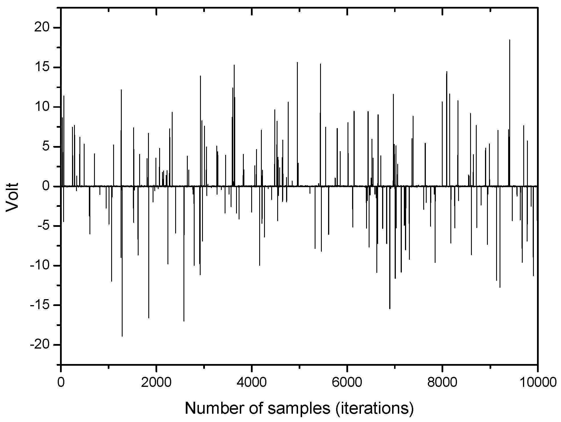
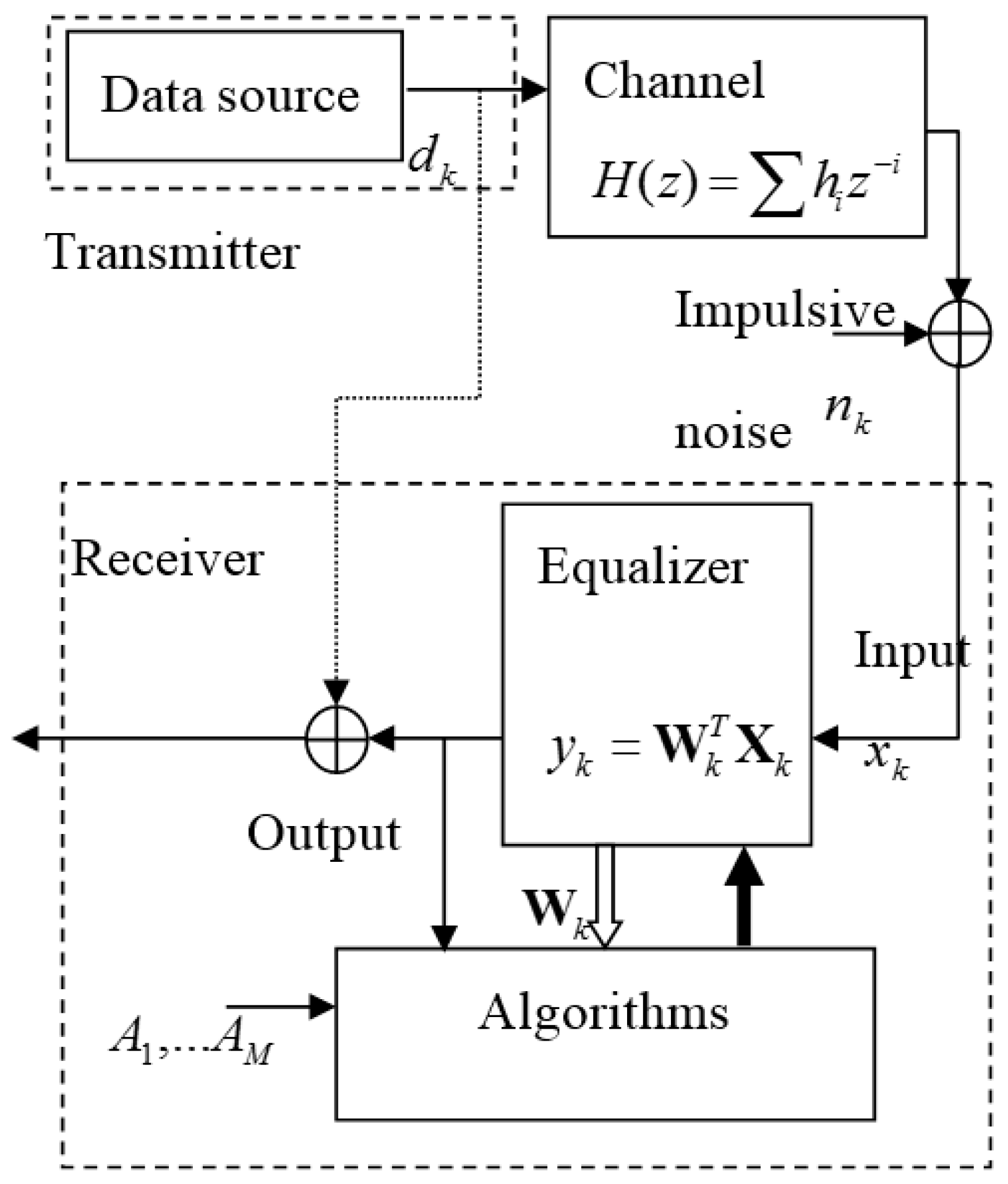
A base-band communication system with multipath fading channel and impulsive noise used in the experiment is depicted in Figure 1. The symbol set in the transmitter is composed of equally probable four symbols (−3, −1, 1, 3). The transmitted symbol is to be distorted by the multipath channel H(z) = 0.26 + 0.93z⁻¹ + 0.26z⁻² [12]. The channel output is added by impulsive noise n_k. The distribution function of n_k, f(n_k) is expressed in

Table 2. Simulation setup and parameter values.

Features	Parameters
The symbol points in the transmitter	$(A_1,A_2,A_3,A_4)=(-3,-1,+1,+3)$
The channel transfer function $H(z)$	$H(z)=0.26+0.93z^{-1}+0.26z^{-2}$
The noise distribution function $f(n_k)$	$f(n_k)=\frac{1-\epsilon }{{\sigma }_{\mathrm{GN}}^{}\sqrt{2\mathsf{\pi }}}\exp [\frac{-n_k{}^2}{2{\sigma }_{\mathrm{GN}}^2}]+\frac{\epsilon }{\sqrt{2\pi ({\sigma }_{\mathrm{GN}}^2+{\sigma }_{\mathrm{IN}}^2)}}\exp [\frac{-n_k{}^2}{2({\sigma }_{\mathrm{GN}}^2+{\sigma }_{\mathrm{IN}}^2)}]$, $\epsilon =0.03$, ${\sigma }_{\mathrm{GN}}^2=0.001$, ${\sigma }_{\mathrm{GN}}^2+{\sigma }_{\mathrm{IN}}^2=50.001$
NNumber of weights	11
4 Step size	${\mu }_{\mathrm{CMA}}=0.000001$, ${\mu }_{\mathrm{LMS}}=0.0002$, ${\mu }_{\mathrm{RMED}}=0.005$
Sample size $N$	$6$
Kernel size $\sigma$	$0.6$

where ${\sigma }_{IN}^2$ is the variance of impulses which are generated according to Poisson process (occurrence rate ε) and ${\sigma }_{GN}^2$ is that of the background Gaussian noise [13]. The simulation setup and parameter values are described in the Figure 1 and the Table 2.

An example of impulsive noise being used in this simulation is depicted in Figure 2.

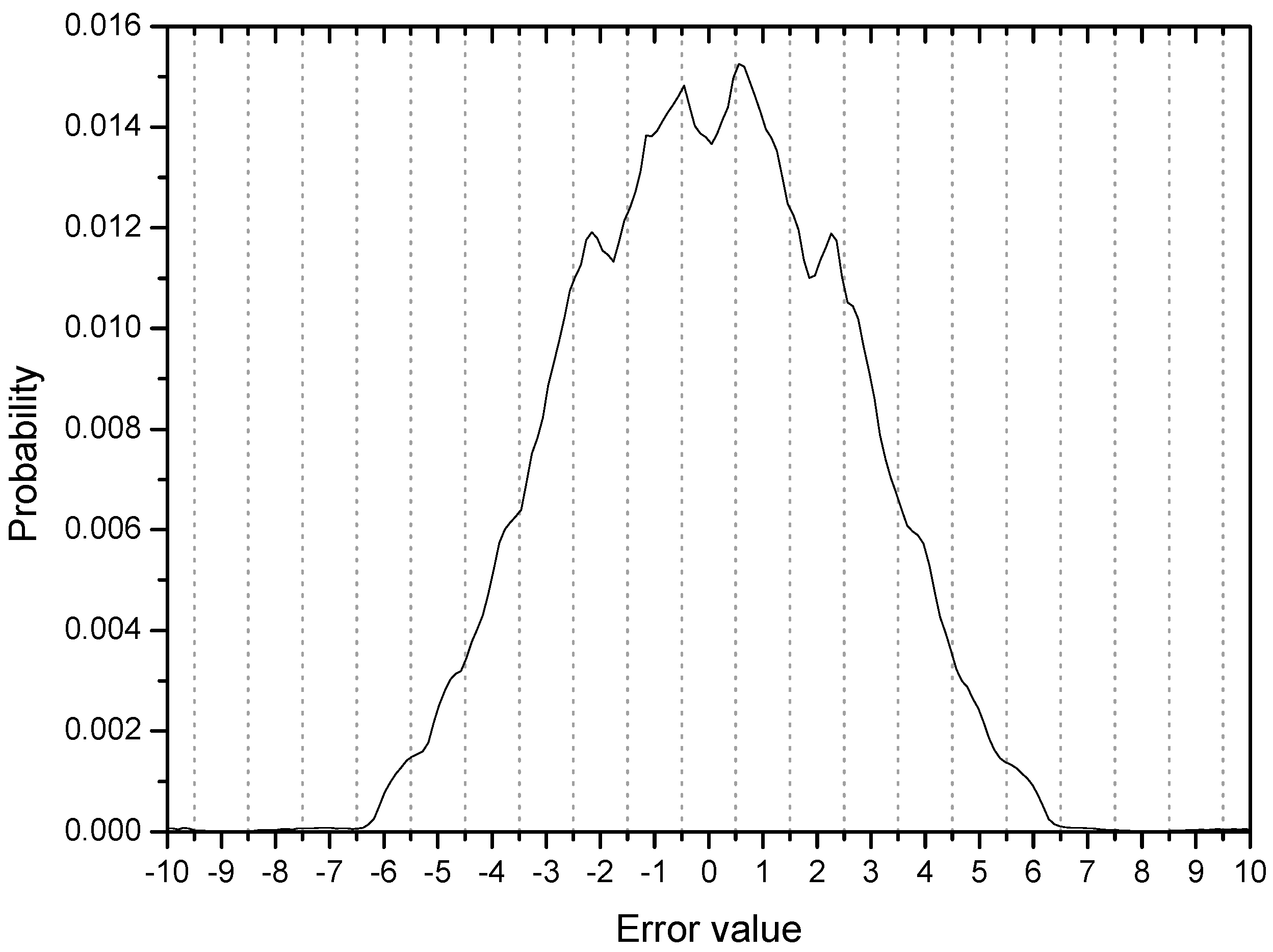
It has in Section 4 been analyzed that U_k is associated with the role of spreading output samples which are clustered to wrong positions due to distorted channel characteristics and V_k is related with moving output samples close to symbol points. This process can be explained through initial-stage investigation of what happens in the error distribution and observing how the distribution of output samples changes in the experimental environment.

Figure 3 shows the error distribution in the initial stage with 200 error samples and ensemble average of 500 runs. Considering the four symbol points are (−3, −1, 1, 3), error values greater than 1.0 are associated with output samples which can be decided as wrong symbols. The cumulative probability of initial output samples placed in the wrong regions in this respect is calculated to be 0.35 from the Figure 3 (35% output samples are not in place). The peaks or ridges in the error distribution are about 6 on each side. This observation may indicate that output samples are clustered or grouped in some regions (two groups are within the correct range but 4 groups are in the incorrect positions on each side of the distribution). 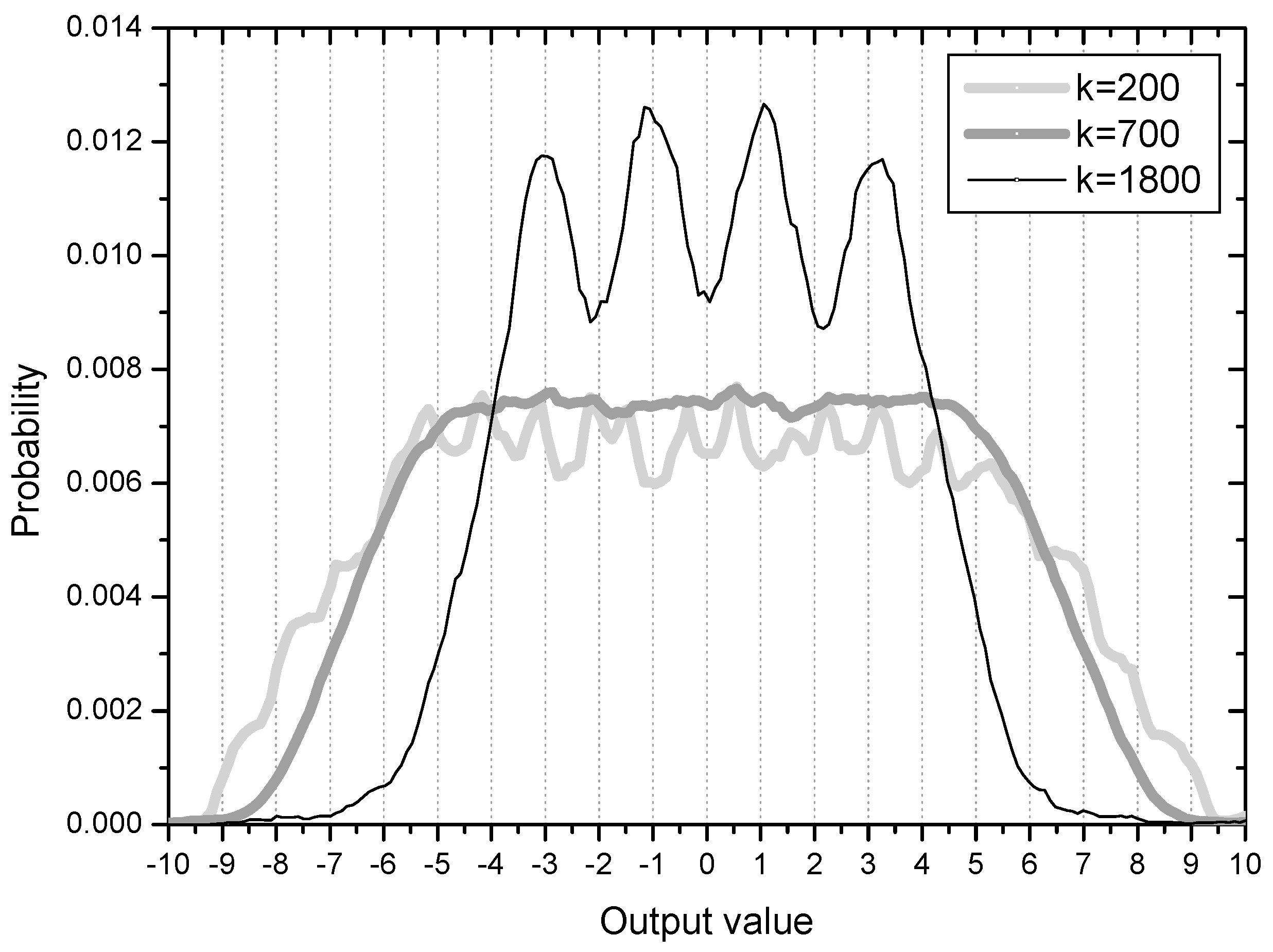This result coincides clearly with the initial output distribution in Figure 4. The output distribution showing about 12 peaks indicates that the initial output samples are clustered into 12 groups mostly located out of place, that is, not around −3, −1, 1, 3.

On the 35% output samples clustered in the wrong symbol regions, the spreading force has a positive effect in order for them in blind search to move out for finding their correct symbol positions. This process is observed in the graph of k = 700 in Figure 4. The output distribution at time k = 700 has an evenly spread shape, indicating that the clustered output samples have moved out and mingled with one another. At the sample time k = 1800 the output samples start to position at their correct symbol areas. From this phase, the force moving output samples close to the symbol points is in effect on lowering steady state MSE.

These results imply that U_k is related with convergence speed and V_k with steady state MSE. To verify this analysis we experiment the proposed algorithm in the following three modes with respect to convergence speed and steady state MSE (we assume that steady state MSE is close to minimum MSE):

$$\mathrm{Mode}1W_{k+1}=W_k-{\mu }_{\mathrm{RMED}}\frac{\partial U_k}{\partial W}\frac{1}{P_U(k)}+{\mu }_{\mathrm{RMED}}\frac{\partial V_k}{\partial W}$$

(30)

$$\mathrm{Mode}2W_{k+1}=W_k-{\mu }_{\mathrm{RMED}}\frac{\partial U_k}{\partial W}+{\mu }_{\mathrm{RMED}}\frac{\partial V_k}{\partial W}\frac{1}{P_V(k)}$$

(31)

$$\mathrm{Mode}3W_{k+1}=W_k-{\mu }_{\mathrm{RMED}}\frac{\partial U_k}{\partial W}\frac{1}{P_U(k)}+{\mu }_{\mathrm{RMED}}\frac{\partial V_k}{\partial W}\frac{1}{P_V(k)}$$

(32)

Mode 1 of RMED-SN algorithm in (30) is for observing changes in initial convergence speed by normalizing only $\raisebox{1ex}{$\partial U_k$}\!\left/ \!\raisebox{-1ex}{$\partial W$}\right.$ by the average power P_U(k) of entropy-input X_i,k compared to the not-normalized RMED. Mode 2 is to observe whether the normalization of $\raisebox{1ex}{$\partial V_k$}\!\left/ \!\raisebox{-1ex}{$\partial W$}\right.$ by P_V(k) of input X_k without managing U_k lowers the steady state MSE of RMED. Finally we see if Mode 3 employing normalization of $\raisebox{1ex}{$\partial U_k$}\!\left/ \!\raisebox{-1ex}{$\partial W$}\right.$ and $\raisebox{1ex}{$\partial V_k$}\!\left/ \!\raisebox{-1ex}{$\partial W$}\right.$ simultaneously yields both of the two performance enhancements; faster convergence and lowered steady state MSE.

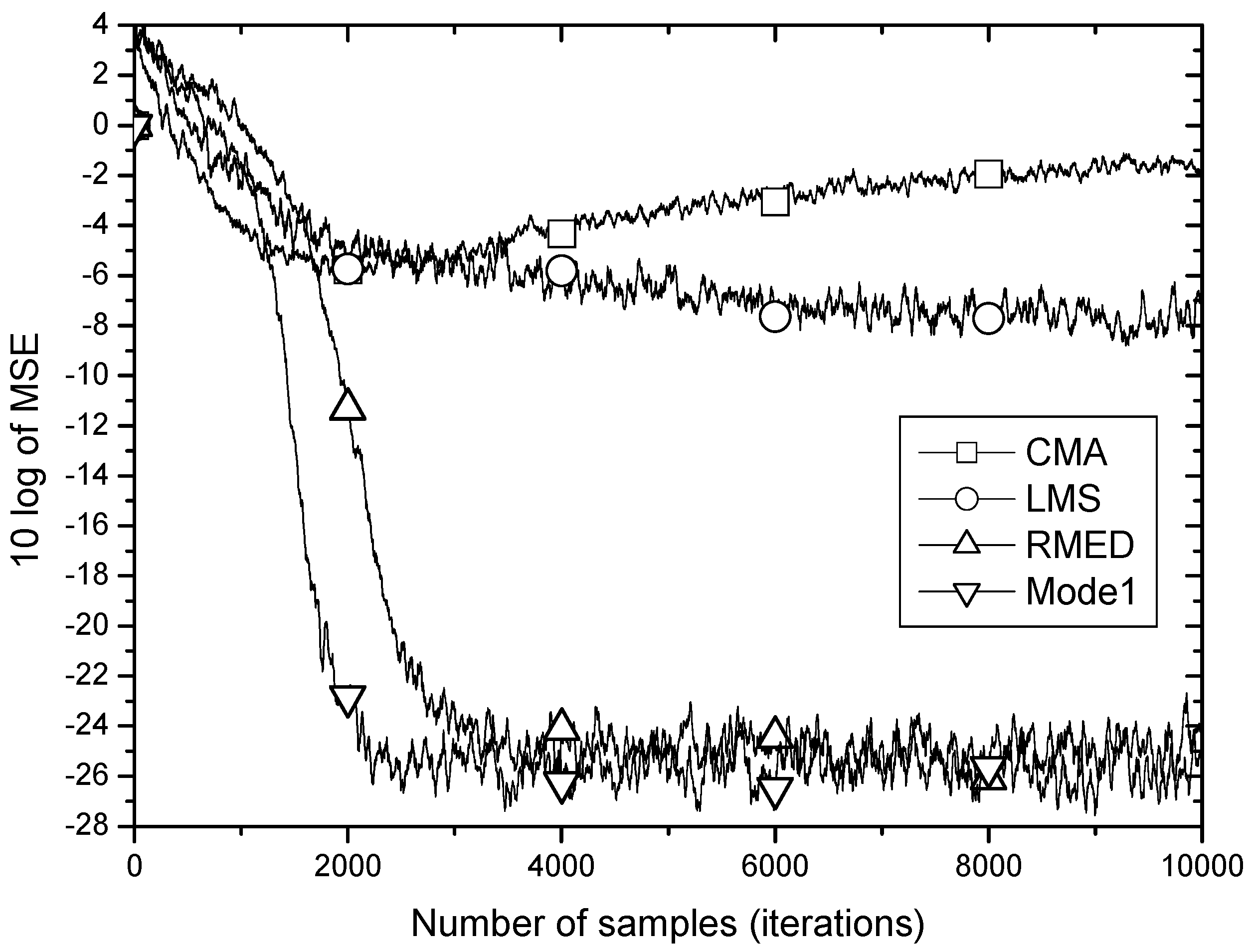
Figure 5 shows the MSE learning performance for CMA, LMS, RMED and Mode 1 of the proposed algorithm. As discussed in Section 2, the learning curves of the MSE-based algorithms, CMA and LMS do not fall down below −6 dB being defeated by the impulsive noise. On the other hand, the RMED and proposed algorithm show a rapid and stable convergence. The difference of convergence speed between RMED and Mode 1 is clearly observed. While the RMED converges in about 4000 samples, the Mode 1 does in about 2000 samples. Therefore, Mode 1 shows faster convergence than the RMED algorithm by 2 times verifying the analysis of the role of $U_k$ since only $\raisebox{1ex}{$\partial U_k$}\!\left/ \!\raisebox{-1ex}{$\partial W$}\right.$ is normalized but $\raisebox{1ex}{$\partial V_k$}\!\left/ \!\raisebox{-1ex}{$\partial W$}\right.$ is not, and we see little difference (about 1 dB) in the steady state MSE.

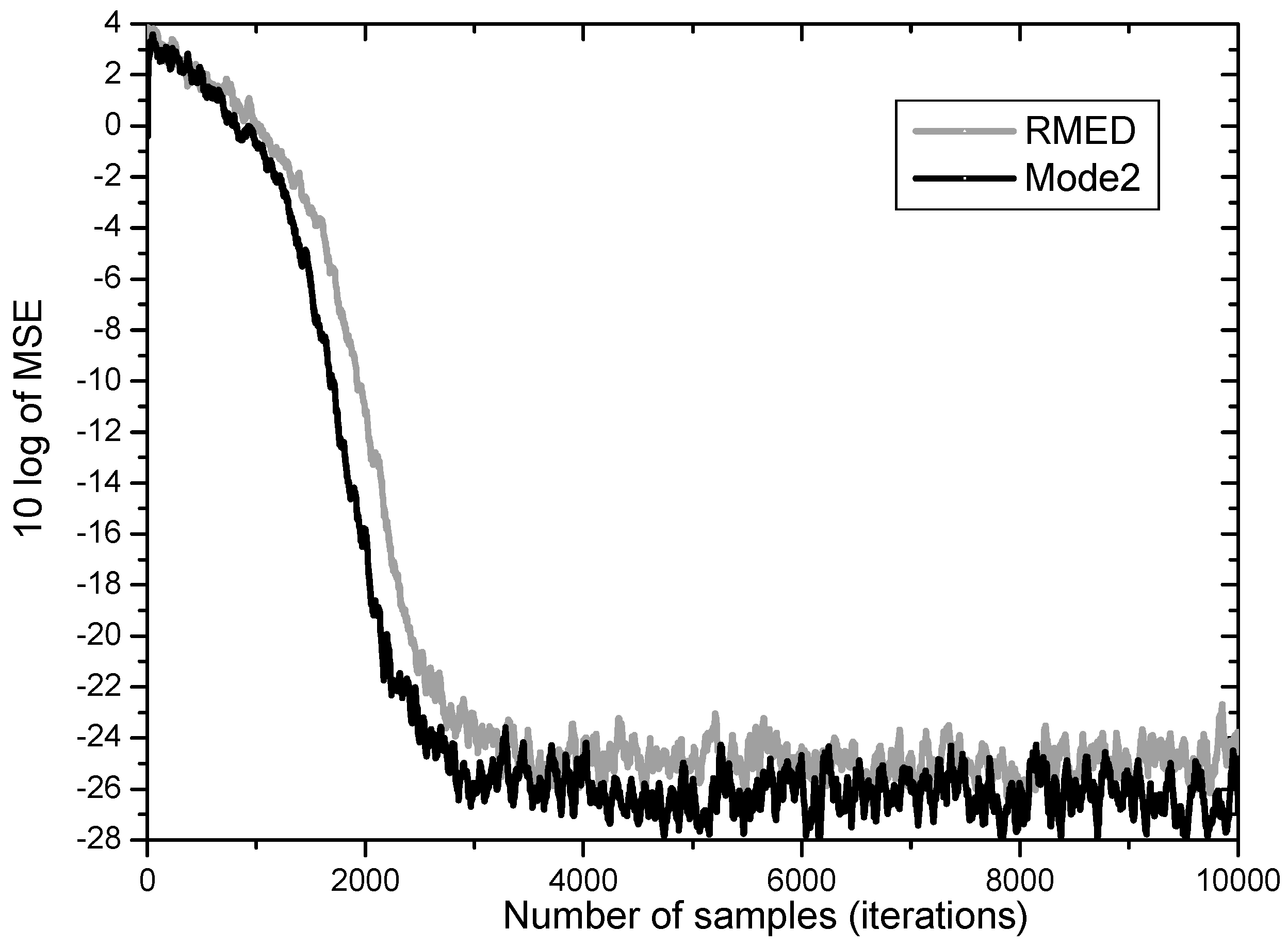
In Figure 6 RMED and Mode 2 are compared. Both algorithms have similar convergence speed with difference of only 500 samples. But after convergence the Mode 2 yields much lower steady state MSE than the original RMED by over 2 dB. These findings indicate that the role of V_k is definitely related with lowering minimum MSE. This is in accordance with the analysis that U_k plays the role of pulling error samples close together.

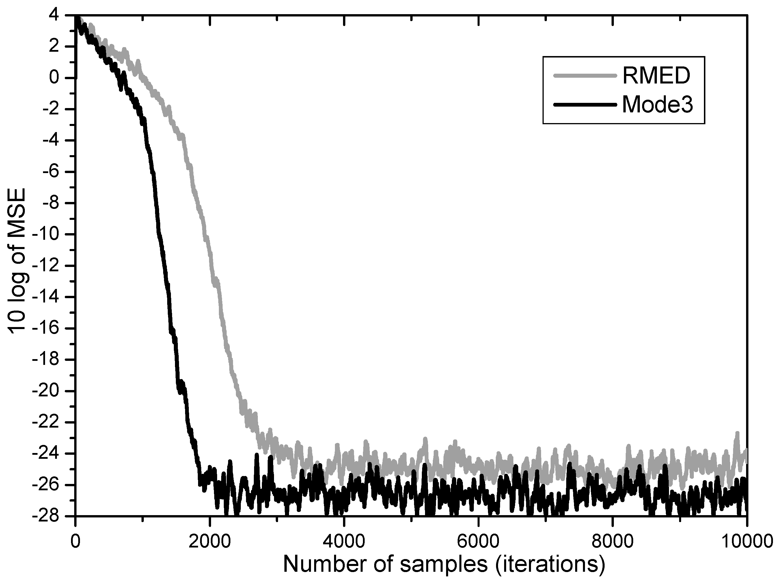
Furthermore, Mode 3 employing normalization of $\raisebox{1ex}{$\partial U_k$}\!\left/ \!\raisebox{-1ex}{$\partial W$}\right.$ and $\raisebox{1ex}{$\partial V_k$}\!\left/ \!\raisebox{-1ex}{$\partial W$}\right.$ simultaneously proves to yield the two merits of performance enhancement revealing increased speed and lowered steady state MSE as depicted in Figure 7. While the RMED converges in about 4000 samples and leaves its steady state MSE at about 25 dB, the Mode 3 converges in about 2000 samples and has about 27 dB of steady state MSE. By employing Mode 3, we obtained faster convergence by about 2 times and lower steady state MSE by over 2 dB.

In Mode 3, it is still not clear whether the normalization to U_k for speeding up the initial convergence may have a negative influence in later iterations, so we try to reduce the U_k normalization gradually after convergence (k ≥ 3000) by using $P_U^{\circ }\left(k\right)$ in place of P_U(k) as:

$$P_U^{\circ }(k)=P_U(k)·c^{k-3000}+(1-c^{k-3000})$$

(33)

where k ≥ 3000 and a constant c is 0 ≤ c ≤ 1.

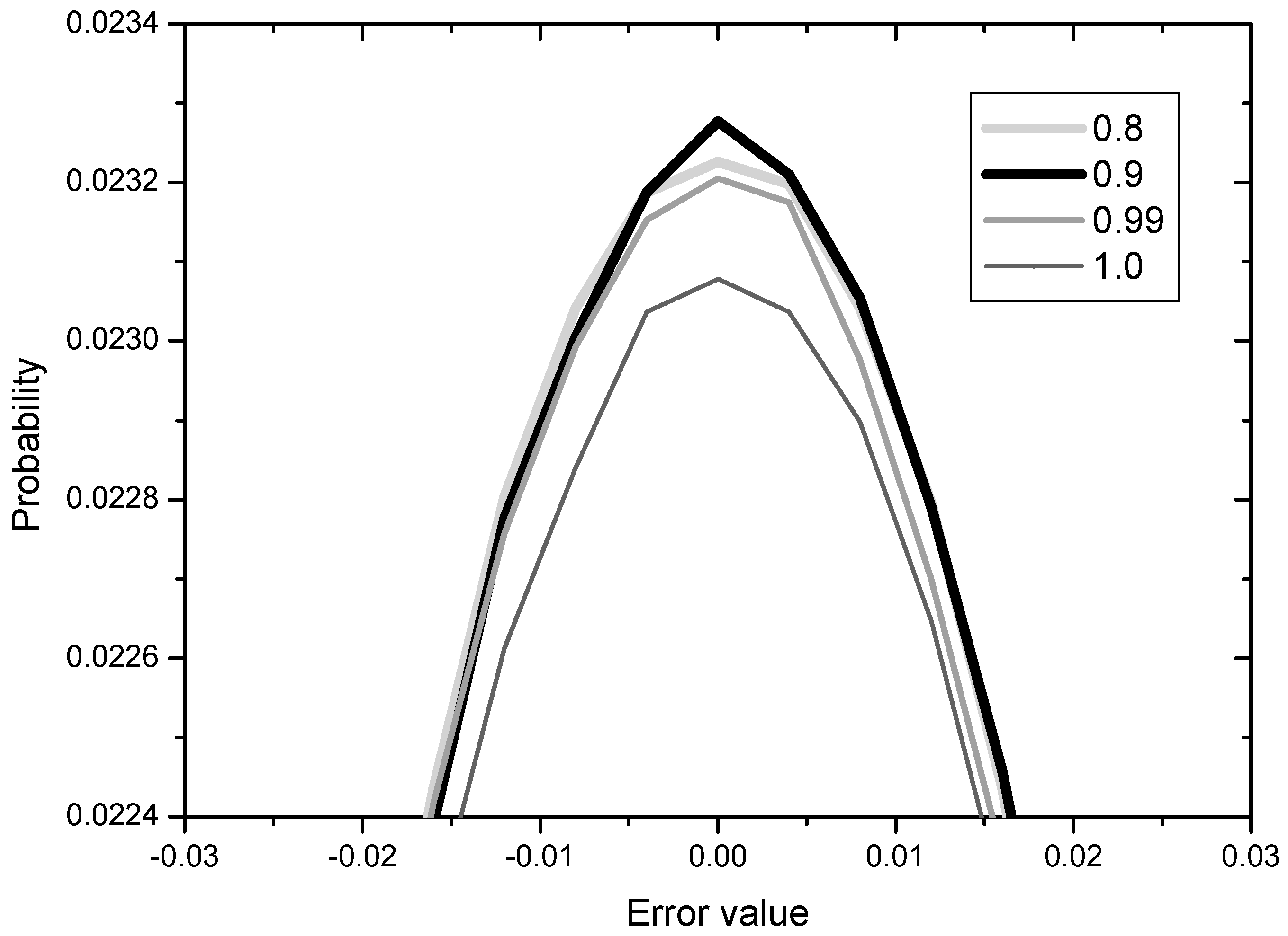
The results for c = 0.8, 0.9, 0.99, 1.0 are shown in Figure 8 in terms of error distribution since the learning curves for the various constant values are not clearly distinguishable.

The value of c in (33) may be related with the degree of gradual reduction in the normalization to U_k, that is, c = 1 indicates no reduction (Mode 3 as it is) and c = 0.8 means comparatively rapid reduction. From the Figure 8, we observe that the error performance becomes better and then worse as the degree of reduction decreases from 0.8 to 1.0. This implies that the gradual reduction of the normalization to U_k is effective but not much. We may conclude that the normalization to U_k for speeding up the initial convergence has a slight negative influence in later iterations and this can be overcome by employing the gradual reduction of the U_k normalization.

7. Conclusions

Minimization of the Euclidean distance between output distribution and Dirac delta function as a performance criterion is known to force the distribution of system output to come to a set of delta functions located at each symbol point. In the analysis of the algorithm RMED developed based on that criterion and recursive gradient estimation, it has been revealed in this paper that the minimization process of the cost function uses its two gradients with different functions; one for U_k that forces spreading of output samples and the other one for V_k that compels output samples to move close to symbol points. In order to verify the roles of U_k and V_k explained in the analysis by controlling U_k and V_k separately, we proposed to normalize $\raisebox{1ex}{$\partial U_k$}\!\left/ \!\raisebox{-1ex}{$\partial W$}\right.$ with the averaged power of entropy-governing input and to normalize $\raisebox{1ex}{$\partial V_k$}\!\left/ \!\raisebox{-1ex}{$\partial W$}\right.$ with that of input. From the results through simulation for the separate normalization of the gradients of RMED in multipath channel equalization under impulsive noise, faster convergence by about two times through normalization of $\raisebox{1ex}{$\partial U_k$}\!\left/ \!\raisebox{-1ex}{$\partial W$}\right.$ and lower steady state MSE by over 2 dB by normalization of $\raisebox{1ex}{$\partial V_k$}\!\left/ \!\raisebox{-1ex}{$\partial W$}\right.$ have been observed. From the analysis and experimental results, we can conclude that U_k is associated with the role of accelerating initial convergence speed by spreading output samples which may have clustered around wrong places in the initial-stage due to channel distortions, and V_k is related with lowering the minimum MSE by pulling error samples close together through the minimization of C_ED,k. Also it can be concluded that through applying normalization to the two factors $\raisebox{1ex}{$\partial U_k$}\!\left/ \!\raisebox{-1ex}{$\partial W$}\right.$ and $\raisebox{1ex}{$\partial V_k$}\!\left/ \!\raisebox{-1ex}{$\partial W$}\right.$ separately with each related input power, significant performance enhancement can be achieved.