1. Introduction
A series of novel quantum processing units (QPUs) has been developed recently based on the principles of adiabatic quantum computing. This computational model uses the time-dependent change in the underlying Hamiltonian to drive the pure-state dynamics of a quantum physical system serving as a quantum computational register [
1,
2]. Ideal operation concludes by preparing the state of the quantum register in the ground state of the driving Hamiltonian at the final time. The designed quantum dynamics rely on the conditions of the adiabatic theorem to ensure the prepared state maps into the lowest energy eigenstate. However, these idealized principles of operation are difficult to realize in practice. One of the reasons is related to the fact that the actual quantum state for the register elements depends on temperature. Besides this, imperfections in the fabrication of the QPU device may introduce undesired couplings between the registers. Given these unavoidable circumstances, it is therefore necessary to ask how well the principles of adiabatic quantum computing suffice for developing applications using current QPU devices.
We focus on the QPU developed by D-Wave Systems, Inc., which represents a special-purpose variant of the adiabatic model limited to a restricted set of Hamiltonians, namely, a traverse-field Ising model [
3,
4]. This restriction imposes a limit on the Hamiltonian interactions driving the dynamics of the register elements during computation. While these limited interactions do not encode the complete range of solutions amenable to adiabatic quantum computing [
5], they are sufficient for a narrow set of special-purpose methods referred to as adiabatic quantum optimization. The defining feature of adiabatic quantum optimization is that it is the final time the Hamiltonian takes the form of an Ising spin-1/2 system, which is isomorphic to a wide variety of conventional optimization problems. The underlying principles of adiabatic quantum computing therefore provide the ability to encode and solve a variety of interesting problems [
6].
The D-Wave QPU has been shown previously to operate far from the ideal conditions for which they were designed but instead lie in a regime more aptly called quantum annealing [
7]. This finite-temperature, open system model is expected to more accurately describe the dynamics underlying the QPU [
8]. Nevertheless, several experimental tests of the D-Wave QPU have been carried out including applications of machine learning, binary classification, protein folding, graph analysis, and network analysis [
9,
10,
11,
12,
13,
14,
15,
16,
17,
18]. Demonstrations of enhanced performance using the D-Wave QPU have been found only for a few selected and highly contrived problem instances [
19,
20,
21]. Thus, there is an outstanding need to find broad classes of applications for which the current hardware offers improvements [
22,
23]. Many such investigations have been based on measuring the time-to-solution for the associated problem, especially with respect to problem size and features [
24]. These metrics emphasize the need to experimentally verify potential claims of quantum-enhanced speedups. Notwithstanding the search for quantum speedups, the fact that the D-Wave QPU computes the solution to any problem accurately, and with high probability, raises the question as to whether the idealized principles of adiabatic quantum optimization are warranted when designing applications and algorithms for this processor. This is an important point in understanding how the D-Wave QPU programming and execution models integrate future applications into existing computing systems [
25,
26,
27].
As a specific example, we consider the application of adiabatic quantum optimization to the problem of recall in a content-addressable memory system [
28]. Content-addressable memory (CAM) represents a memory structure in which key-value data is recalled based on its value as opposed to its key [
29]. Unlike random-access memory (RAM), which uses an organized hierarchy of keys to recall a value, CAM uses the value to recall the key within an otherwise unorganized list. This difference in operation is apparent in the ways in which CAM and RAM are typically used. For example, the CAM paradigm is especially useful for interacting with sets of key-value pairs that are unsorted or unorganized [
30]. This includes networking applications such as switching, where incoming packets are routed to outgoing ports based on header address information stored as the key-value pair (port, address) [
31]. Similarly, CAM systems are also used for translation lookaside buffers (TLB’s), which are a critical part of modern computer memory hierarchies that enables fast caching.
CAM recall using adiabatic quantum computing is based on finding the energetic minimum of a Ising model constructed from a database of known key-value pairs [
28]. Under ideal conditions, the energetic minimum within this Ising model energy landscape encodes the association between a sought-after key-value pair. This association between the key-value pair and energetic minima is also what underlies existing CAM recall methods based on neural networks [
32]. Although the physics of conventional neural networks are fundamentally different from quantum physical systems, the principles of operation for both types of memory systems are the same while their performance is not [
33,
34]. For example, a prominent concern in neural network methods for CAM recall is avoiding interference between stored memories [
35,
36]. Interference limits the number of memories that can be accurately recalled from
n-bits of storage, i.e., the so-called memory capacity. Depending on the encoding methods (learning rules) applied, conventional memory recall methods yield logarithmic and polynomial capacities [
32,
36,
37].
Previously, Nishimori and Nonomura found that a quantum Ising model demonstrates many of the same statistical features as the conventional Ising spin system [
33]. Most notably, this includes a phase separation between the memory-retrieval and spin-glass phase near a pattern to spin ratio
for vanishing transverse field, which mirrors earlier results from McEliece et al. for classical spin systems [
36]. However, Santra et al. have shown recently that the capacity for memory recall using adiabatic quantum optimization can be exponential in the size of the memory [
34]. This remarkable enhancement in the capacity suggests that the quantum dynamics play an important role in mitigating interference. However, whether this enhancement can be observed depends on the versatility of the underlying device to overcome computational bottlenecks. For example, Knysh has shown recently that many binary optimization problems mapped into the quantum Ising model become limited by the appearance of multiple energy gaps in the quantum computational landscape [
38].
We previously verified the principles of CAM recall by adiabatic quantum optimization using numerical simulations to investigate the pure-state dynamics of a small memory system [
28]. Through simulations of the quantum dynamics, we showed that specific key-value associations could be recovered when the ground state of an encoded Ising model Hamiltonian was prepared by adiabatic quantum optimization. The related problem of pattern recognition, in which a single noisy value is correctly recovered, has been validated experimentally by Neigovzen et al. using nuclear magnetic resonance (NMR) platforms [
10]. In this contribution, we experimentally test the performance of CAM recall using the D-Wave QPU and the principles of adiabatic quantum optimization. We compare different methods of expressing the association between key-value pairs and we test the accuracy available by using different learning rules. Our results experimentally validate the ability for the QPU to recall stored memories within the context of adiabatic quantum optimization but they also highlight the sensitivity of the application to potential hardware limitations. Our analysis has been restricted to a pure-state model, and future studies using more sophisticated quantum annealing models may be able to improve upon these results.
2. CAM Recall Using Adiabatic Quantum Optimization
A CAM system stores the association between a key
k and a value
v and recalls this association by retrieving
k when given an exact or an approximate value for
v. A CAM system should recall the key that is closest to the matching value stored in memory. This is in contrast to random access memory (RAM), which may also store a key-value pair
but recalls whatever value is associated with the provided key, e.g., a memory address. We formalize the CAM recall problem as follows: given a set
of
m key-value pairs that are each of total length
n, recall with probability of success
the key
corresponding to the known value
. The order by which labels are assigned to the
m memories is arbitrary and, therefore, recall of the pair
expresses the general problem. Elements
and
use the bipolar encoding
. Our definition of the problem has introduced the success probability
to account for those solvers that may only be probabilistically correct. As explained below, the implementation of adiabatic quantum optimization realized by the D-Wave QPU fits such a probabilistic model. In practice, it is necessary to quantify recall performance with respect to the statistical behavior of an ensemble of identically prepared instances.
As discussed in the introduction, adiabatic quantum optimization (AQO) is an algorithmic variant for finding the global minimum of an objective function. The objective function must be expressed as a Hamiltonian whose lowest energy eigenstate, i.e., ground state, defines a valid solution for the encoded optimization problem. By the nature of being the lowest energy state, this solution corresponds to the minimizing argument of the objective function. Adiabatic quantum optimization specifies the objective Hamiltonian as part of the time-dependent evolution of the underlying quantum register, where the idealized equation of motion is given by Schrodinger’s equation and the initial boundary condition for the register state is defined as the known ground state of a more easily solved Hamiltonian. During evolution, the initial Hamiltonian is slowly deformed, i.e., adiabaticially, to the Hamiltonian expressing the objective function. Completion of the evolution prepares the quantum register as a ground state of the final Hamiltonian. Because the final Hamiltonian expresses the original objective function, the value of the quantum register similarly represents a valid solution for the optimization problem. We will use this idealized model for describing the behavior of the D-Wave QPU.
We encode a CAM recall problem into the AQO solver by storing all key-value pairs in a set
M into the coupling weights of an Ising Hamiltonian
where
is the state of the
i-th spin variable. The real-valued weights
are set according to a learning rule that we specify in detail below. The parameter
represents a vector of real-valued biases that breaks the quadratic symmetry of the Hamiltonian according to the specified input value
. By design, the memories stored in the weights of the Ising model represent stable fixed points within the energy landscape. In the absence of bias
, these states form a degenerate ground state manifold for the spin system. It is the presence of the linear bias term that breaks this symmetry and lowers the energy of the sought-after memory. The non-zero value of
plays an important role in determining the probability for recall success. However, in the limit that
exceeds some critical value, then the biased value
will generate an unexpected fixed-point for the Ising model. In this scenario, the input value is then recalled as opposed to stored memory. This critical value can be calculated based on the Hamming distance between the stored memories [
28,
34].
For a given problem instance, we recover the lowest energy eigenstate of
using AQO. The time-dependent Hamiltonian that evolves the state of the quantum register is defined as
where the schedules
and
control the time evolution and satisfy the boundary conditions
and
given the (adiabatic) evolution time
T. The state of the quantum register is initialized as the ground state of the initial Hamiltonian,
, where
is the transverse-field operator and
is the Pauli bit-flip operator for the
i-th qubit and
is the identity operator on
n qubits. The non-degenerate ground state of this initial Hamiltonian is a uniform superposition of all possible computational basis states with energy—
n. The state of the register at time
t is
and is given by the Schrodinger equation,
over the range
. Under adiabatic quantum dynamics, the register state will be in the ground state of the Hamiltonian
at the final time
. Measuring prepared state in the computational basis yields an
n-bit string
. This classical spin configuration represents the solution to the CAM recall problem, i.e.,
.
The probability that the register is prepared in the ground state of the Hamiltonian is strongly influenced by whether the quantum dynamics underlying the register evolution was sufficiently slow relative to internal dynamical timescales. A leading order error in AQO arises from excitations to higher-lying energy eigenstates. These transitions occur when the instantaneous energy gap between the ground and (first) excited-state manifold becomes small relative to the inverse of the evolution time. The time complexity of this probabilistic algorithm is thus determined by the shortest evolutionary period T needed to obtain a probability to be in the ground state. However, this value is not arbitrary as the probability of success depends on the energy gap for the specific key-value pairs stored in the Hamiltonian according to the elected learning rule. The implicit dependence of the minimal evolution time, necessary to ensure the adiabatic theorem for a specific problem instance, is a well-known challenge for adiabatic quantum computing.
Given a computed solution
, we quantify the accuracy of recall by comparing the measured spin string
with the expected state
as the inner product
. Perfectly accurate recall coincides with a maximal value of the inner product
for the bipolar encoding. For the criterion of perfect recall, any other value for
c is considered a recall failure. Under this criterion, we may then calculate the average accuracy for an ensemble of
N trials with
the results of the
i-th trial. We quantify accuracy for perfect recall as
with the Kronecker
only if
and 0 otherwise. This measure of accuracy is the frequency by which the sought-after memory is found exactly over all trials.
3. Experimental Validation of CAM Recall
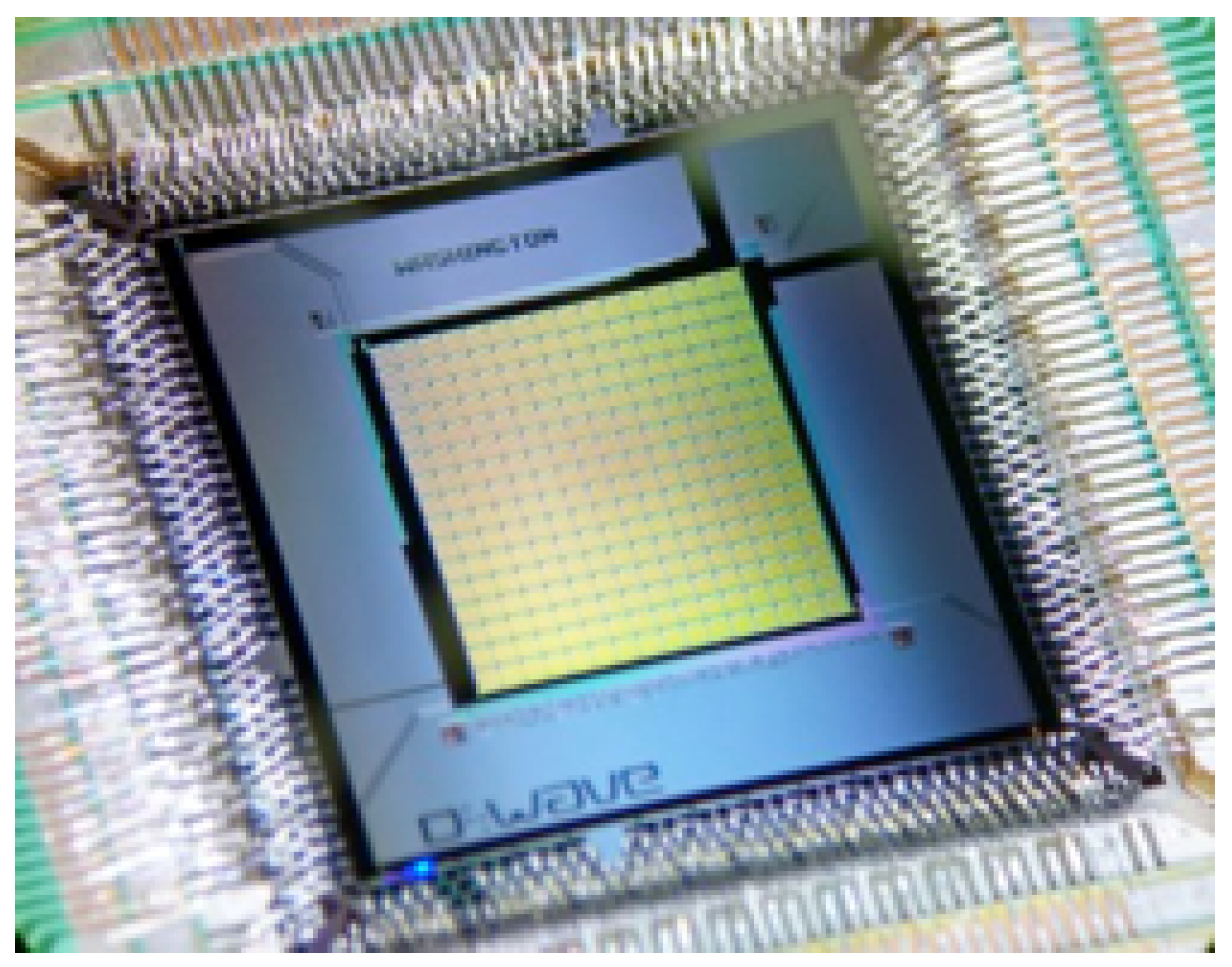
We have performed experimental tests to validate the principles of CAM recall using adiabatic quantum optimization implemented in the 1152-qubit D-Wave QPU [
24]. Variants of this device have been installed in several third-party locations, and our experimental results were acquired using the D-Wave QPU housed at the NASA Ames Research Center. A photograph of an example D-Wave QPU is shown in
Figure 1.
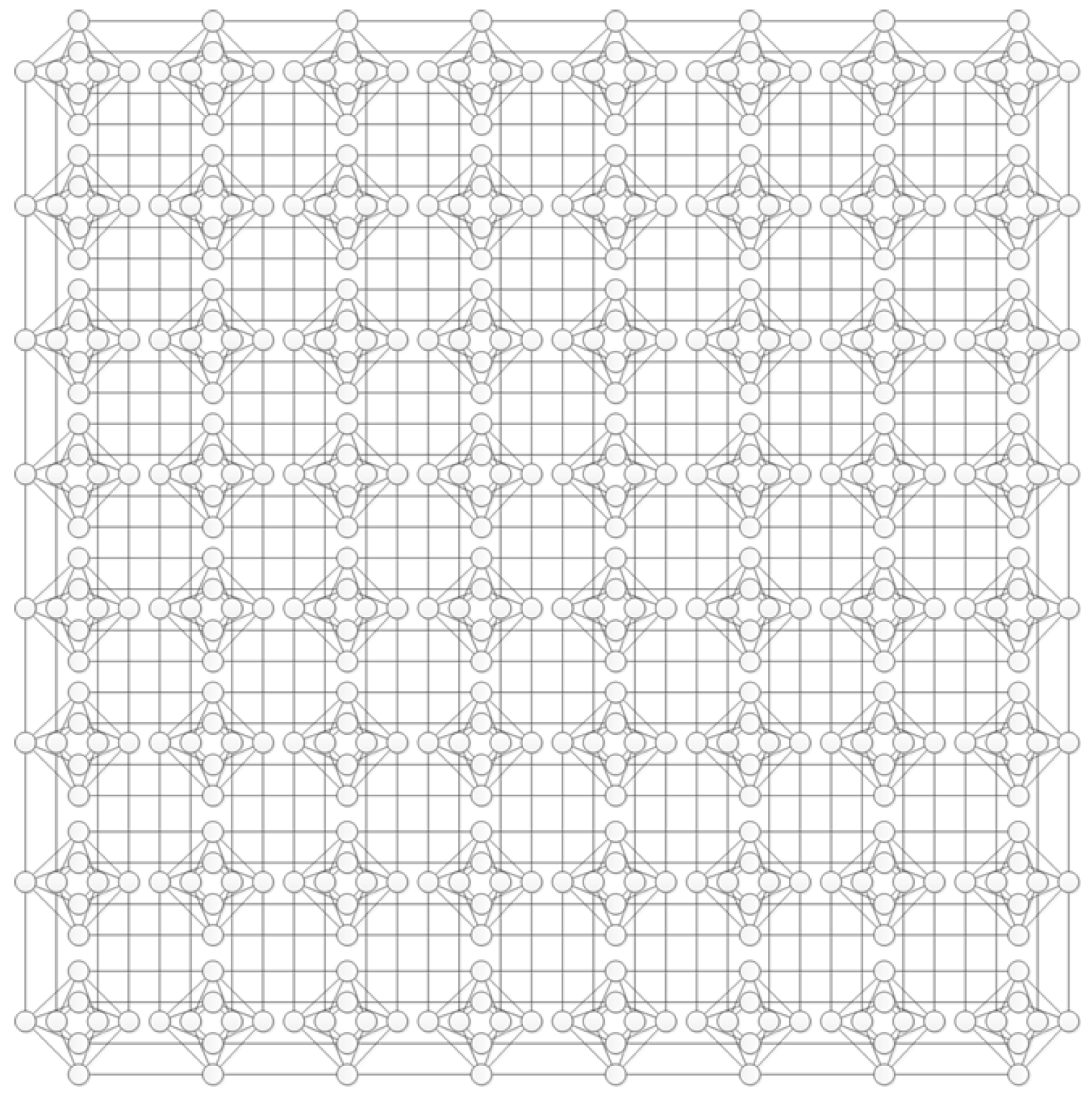
The D-Wave QPU provides an implementation adiabatic quantum optimization model with several known hardware constraints. Foremost are restrictions on the available Ising model Hamiltonian. In particular, the processor hardware is constructed from an array of interacting superconducting Josephson junctions laid out in a square grid of bipartite graphs known as the Chimera graph. A graphical model of this connectivity is shown in
Figure 2. These limitations on hardware connectivity restrict which qubits can interact together. The Chimera layout permits interactions of each qubit with only six neighbors, and only five neighbors for qubits on the edge. The limited connectivity between hardware register elements can be partially overcome by forming chains of physical qubits to represent so-called logical qubits. The mapping from a set of logical qubits to set of physical qubits represents the problem of minor graph embedding, which seeks a representation of the connectivity for the logical Ising Hamiltonian within the physical hardware. Many different methods have been developed for solving the minor graph embedding within the context of the Chimera target graph [
39,
40,
41,
42,
43]. We use a deterministic method for mapping a complete graph into the Chimera layout that is known to provide the least overhead with respect to number of physical qubits and, therefore, enables us to test the largest problem sizes available within this device [
40].
In addition to the embedding method, other programming choices for the D-Wave QPU include the schedule for annealing the system to the final Hamiltonian, which is characterized by the temporal waveform and its duration. The available hardware control systems restrict these options to pre-defined forms and ranges. Execution of the program within the hardware also requires pre-processing steps to initialize the electronic control system and construct the analog signals applied to the quantum chip. These steps include the time required to initialize the programmable magnetic memory (PMM) that is used as the control lines into the super-cooled processor. Technical details about the electronic programming process are available in the relevant literature [
44], but it suffices to note that these steps contribute a near constant time cost to the total for the execution model [
27].
3.1. Problem Instances
A CAM problem is specified by the set of memories M, a sought memory , and a success rate . Our tests focus on evaluating the ability to perform CAM recall using AQO and, therefore, we identify values for in which accurate recall is possible. We sample from a set of problem instances defined by stored memories that correspond to known key-value pairs. For each sample, we choose one of the known key-value pairs as the sought-after association. The pairs are represented as bipolar strings of length n with the first part of the string acting as the key and the remainder as the value. We test cases with a key length and a value length of Sets of memories are characterized as being orthogonal or non-orthogonal. For orthogonal memory sets, all key strings within the set are mutually orthogonal and all value strings are mutually orthogonal. There is no guarantee of orthogonality between any of the keys and values. There can only be n orthogonal vectors in an n-dimensional vector space, and the number of memories generated is limited to the length of the keys or the length of the values. For non-orthogonal memory sets, the only restriction on these randomly generated memories is that the keys and values were unique, such that the number of available memory sets was much greater. Thus, the Hamming distance between any two random keys or values would vary from 1 to or , respectively. We test these instances with respect to statistical sampling derived from running multiple problem instances and we record an average accuracy to score the performance. The performance of CAM recall using AQO is measured by collecting statistics on ensembles of problems given different specifications for the memories and the learning rules.
We reduce a CAM recall problem instance to an AQO instance by mapping the set of memories
M into the Ising Hamiltonian. This is accomplished by encoding the memories into the Ising weight matrix using one of several possible learning rules. A learning rule is a deterministic mapping defined over the set of possible input maps into the real-valued weight coefficients. We investigate the use of several specific mappings well known from the neural network community, namely, the Hebb and projection learning rules, which have been studied previously within the context of Hopfield neural networks. These learning rules are typically used in applications of pattern matching, for which the association is between a value and itself, e.g., to identify a pattern based on partial information. Such pattern matching applications make use of data structures represented by complete graphs. A complete graph structure is sufficient for CAM recall but it is not clear that this graph structure is necessary for an association defined by a bipartite relationship. Due to the connectivity constraints within the D-Wave QPU, we also use variants of these learning rule that take advantage of the bipartite structural relationship between the key and value. This changes the original problem with the intent of being easier to map to the hardware graph while keeping the stored memories as energetic minima. The bipartite structure is especially appealing due to ease of embedding into the hardware graph [
42,
43]. Reducing the encoded interactions between qubits also reduces interference between stored memories. We provide specifications for all three learning rules below.
Given key-value pairs as in Equation (
1), the Hebb rule is defined as [
35]
where
and
n is the length of
. When building the weight matrix
W for a bipartite structure, square diagonal blocks were zeroed out corresponding to the key length and value length. If the length of the keys is
and the length of the values is
, with
, then the submatrix from rows and columns 1 to
is replaced with a zero matrix as is the submatrix from rows and columns
to
n. The off-diagonal blocks then satisfy the original definition of the Hebb rule given in [
32],
where
and
. The final weight matrix for the bipartite Hebb rule is
The second learning rule used is the projection rule [
37]. The projection rule is expected to be an improvement over the Hebb rule because it is based on decorrelating the memory set prior to encoding the weight values. This has the result of minimizing the effect of crosstalk, i.e., interference, between stored memories. Beginning with
M as defined in Equation (
1), the projection rule is given as
where
and
is the pseudo-inverse. As with the Hebb rule, square diagonal blocks are zeroed out to create the bipartite projection rule. This conjecture is supported by empirical evidence below. This third rule is a bipartite projection rule and it is based on the definition in [
32],
where
and
, with
W built as in Equation (
9).
All definitions of the learning rules above allow for weight coefficients that can have a magnitude that scales with . For large values of n, this magnitude can become too small for accurate representation by the D-Wave QPU controls, which are frequently cited as being limited to 4–5 bits of precision. We counter this by scaling values of the weight matrix to better fit into the defined control range of for the QPU. This is done by finding the largest value in the matrix and scaling the matrix by . The latter choice of supported the requirement that intra-chain coupling be much larger than any of the stored weights and was found to improve the observed recall accuracy for several test problems without this scaling.
3.2. Experimental Setup
Our experimental setup uses the Hebb rule as the baseline for recall accuracy. In general, there are 3 parameters varied when selecting the test problems. These parameters are the size of the logical system
n, the number of stored memories
m, and the applied bias
. The orthogonality of the memories is also specified but this case was not of interest beyond the initial testing reported below. Because CAM recall using orthogonal memories is expected to be well behaved, we use that case to test the fundamental performance of the D-Wave processor to recall stored memories. The remaining parameters are chosen from the following sets respectively,
and
For each parameter combination
, 100 problem instances are randomly generated as specified in
Section 3.1 and utilizing one of the learning rules to encode the memories into a weight matrix. Each selected problem instance is then programmed and executed
times on the D-Wave QPU to calculate the average recall accuracy
c.
Executing these programs on D-Wave QPU requires embedding the logical Ising Hamiltonian generated from Equation (
2) into the physical hardware. For our testing purposes, we use the embedding function
find_embedding provided by the D-Wave SAPI library to find a mapping from the logical qubits to the physical qubits. The SAPI
find_embedding method relies on random number generation, and to remove a source of variability, the seed parameter was set to 0 for all tests. The resulting map is then used by the
embed_problem function along with the weight matrix to set the coupling values between qubits and bias values on the qubits. The bias values encode the memory that is to be recalled. Additionally, a strong coupling value of
is set between physical qubits representing the same logical qubit. This complete problem specification is sent to the D-Wave machine using the
solve_ising function with an anneal time of 20
s and the number of reads set to
. The resulting spin configurations are unmapped using the
unembed_answer function. This provides a list of candidate solutions for the CAM recall instance and calculating the accuracy requires searching through this list and counting up the number of correct solutions. This accuracy is averaged over 100 different problem instances. In addition to accuracy, the times to embed the problem and run it on D-Wave are collected and averaged. While we have seen some variability in recall accuracy with changes in anneal time, we do not report on those results below, preferring to focus our analysis on a fixed value of program duration.
Experimental runs are carried out using the D-Wave DW2X processor installed at NASA Quail. This processor has 1097 active qubits laid out in a faulty Chimera connectivity pattern. Data is archived locally and post-processed to generate the results presented in the next section. The results presented were collected in August and September of 2016 [
27].
4. Experimental Results
Accuracy results for CAM recall with orthogonal memories and varying memory sizes are presented in
Figure 3 with plots labeled by
H for the Hebb rule,
P for the projection rule, and
for the bipartite projection rule. We exclude results for other rule definitions because their recall accuracy was typically lower than
P and
.
Figure 3 plots the recall accuracy with respect to the logical key-value size
n, and each line shows the results for a different applied bias
. These results show that the D-Wave QPU is able to perform CAM recall with very high accuracy in the presence of applied bias. In the absence of the bias necessary to select a specific key-value pair, the accuracy is approximately the likelihood of observing any one of the
m orthogonal ground states. We find that the accuracy for recall in a small memory set
quickly increases to one when the bias is increased to a non-zero value. For a small number of logical spins, we observe perfect accuracy in the learning rules with only slight deviations. This behavior is expected for orthogonal memories due to a lack of interference during memory storage. However, as the memory size
m increases, the accuracy decreases for moderate and large bias values. This decrease correlates with an increase in the size of the key-value pair with the largest deviation occurring at the largest value of
. It is important to note that the recall accuracy depends on the learning rule with the bipartite projection rule demonstrating the best average behavior across all test instances. We note there is an unexpected dip in accuracy in
Figure 3a. This is due to several of the tests using random sets of orthogonal memories under the
rule reporting zero recall accuracy for
, an indication that the processor did not exhibit perfect recovery of the sought after memory. Subsequent testing with larger problem sizes yielded perfect accuracy. We speculate this may be due to numerical instabilities in the
rule for low memory capacities as this anomalous dip does not arise for either the
H or
P rules or for larger set sizes.
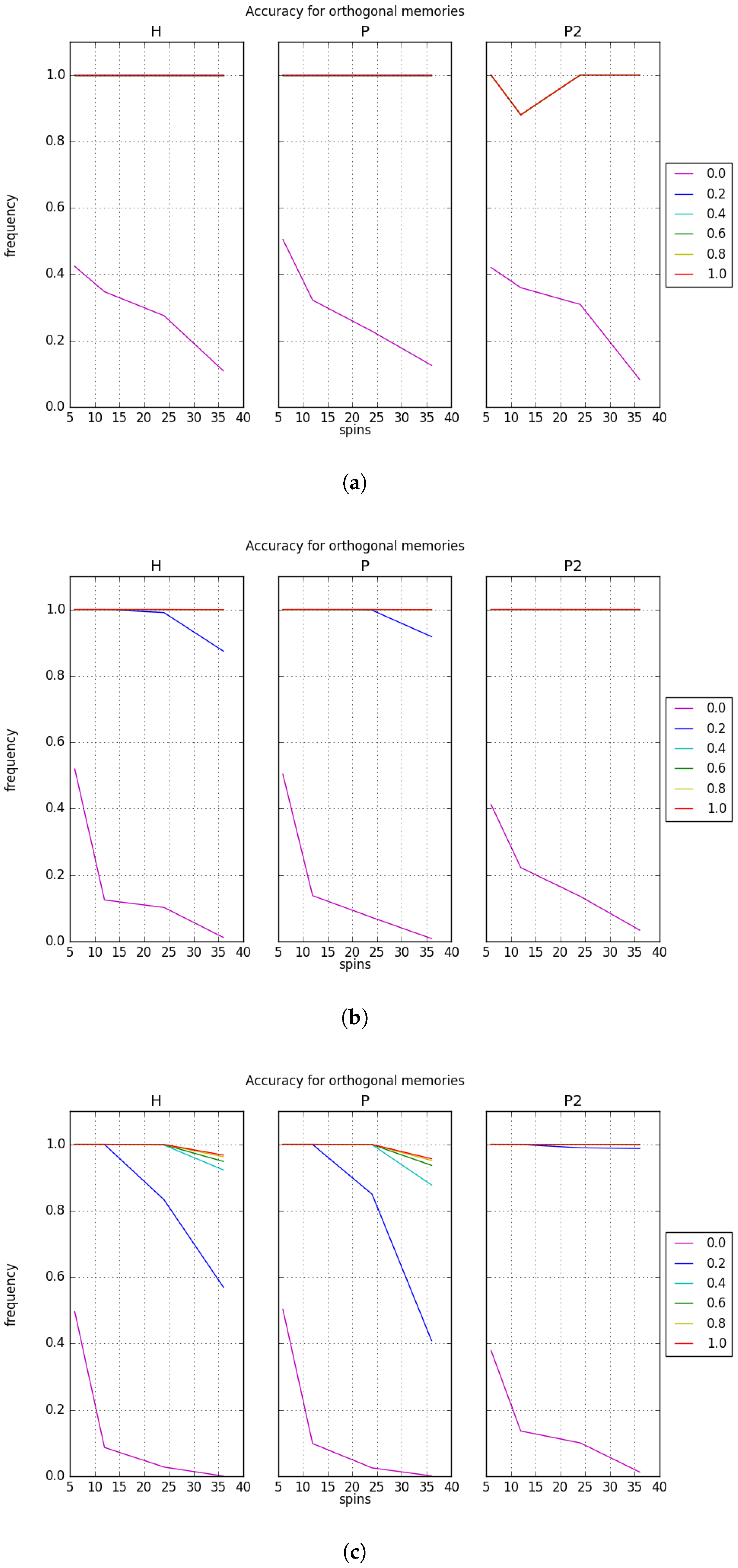
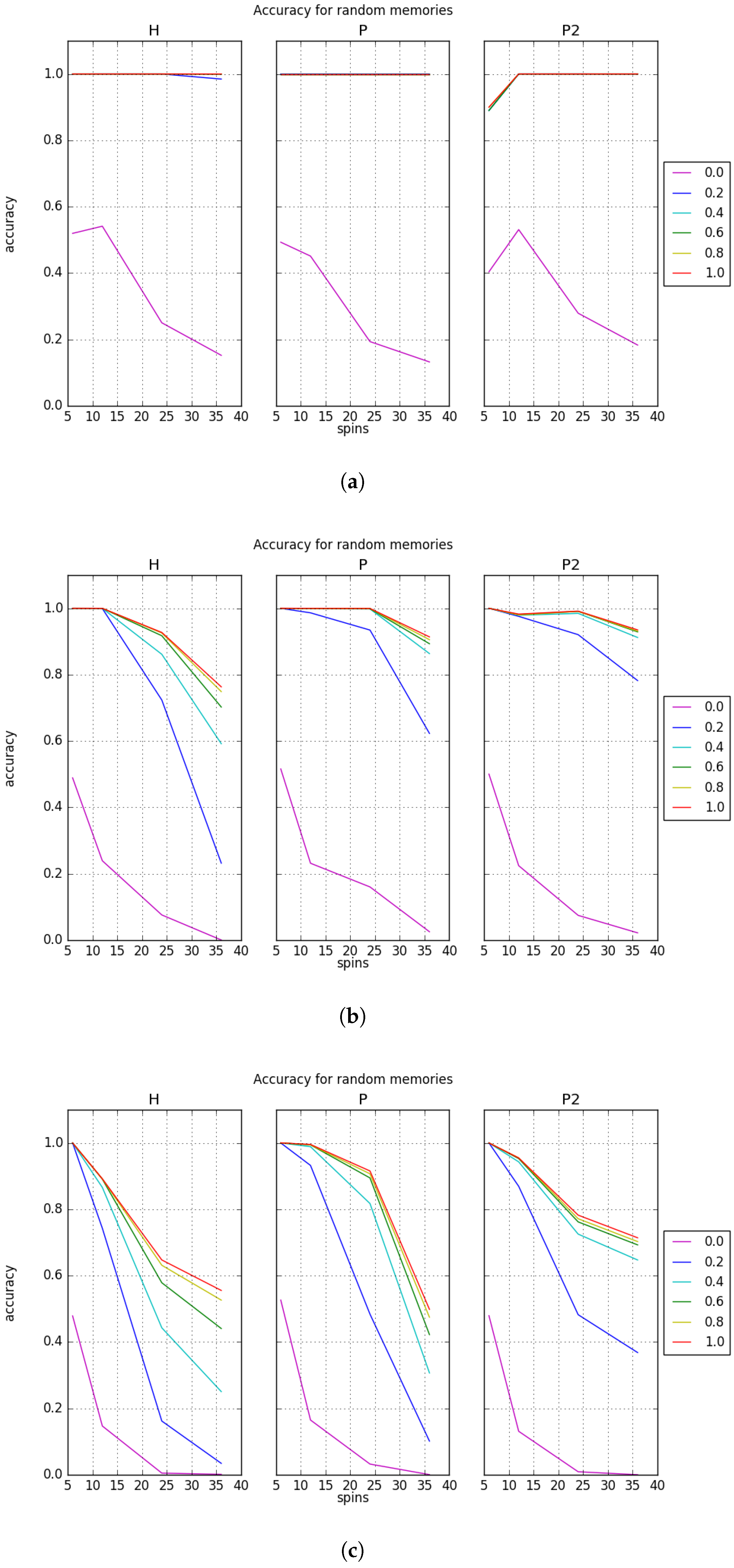
Accuracy results for CAM recall with random memories and varying capacity are presented in
Figure 4 with respect to the number of logical spins. These plots show the recall accuracy as a function of the logical problem size, and each line shows the results for a different applied bias. Plots for the random memories cover a wider range of spins and capacities than the orthogonal memories due to fewer restrictions in their method of generation as discussed in
Section 3.1.
The first observation for results with random memories is that the D-Wave machine can still perform CAM recall but with varying levels of success. As can be seen, the recall accuracy is influenced by several factors. Most striking is the effect the memory capacity has on recall accuracy. The recall accuracy is nearly perfect for all rules and biases in
Figure 4a which corresponds to a capacity of
. However, as the capacity increases, the accuracy decreases to under
for the large problem sizes, as shown in
Figure 4c. The expectation is that the greater the number of memories stored relative to the system size, the greater the interference the memories inflict on each other. The number of local minima is therefore increased while the basins of attraction decrease in radius. As a result, recalling the correct memory becomes more difficult [
28].
Compared to the near perfect recall behavior shown in
Figure 4a, the other plots demonstrate that the choice of learning rule affects the recall accuracy. In particular, the uses of the projection rules
P and
generally perform better than the Hebb rule
H. We believe this indicates that the projection rule alters the underlying energy surface, a behavior that has also been observed in the case of conventional neural networks [
32]. In particular, the projection rule generally performs the best among all rules tested here except when the number of spins reaches 32. There is a sharp drop in recall accuracy at this point for capacities above
though it is most dramatic in
Figure 4b. The projection rule performance even descends below that of
H for some bias values.
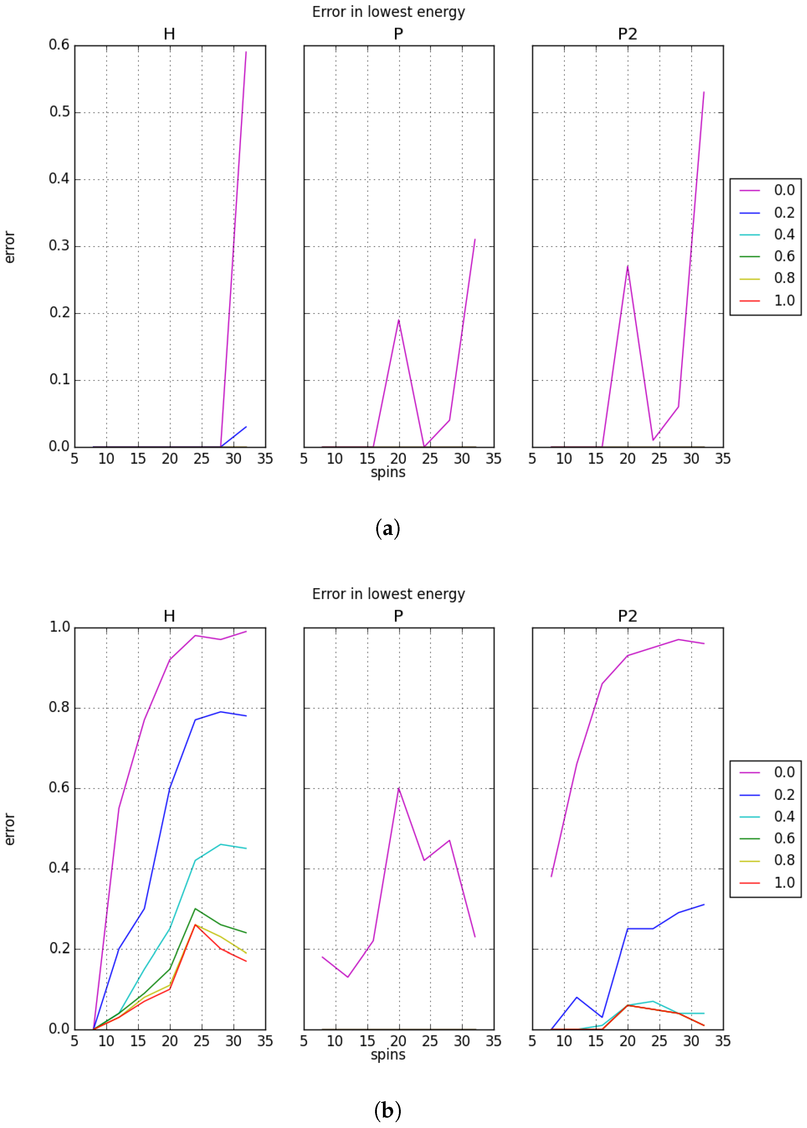
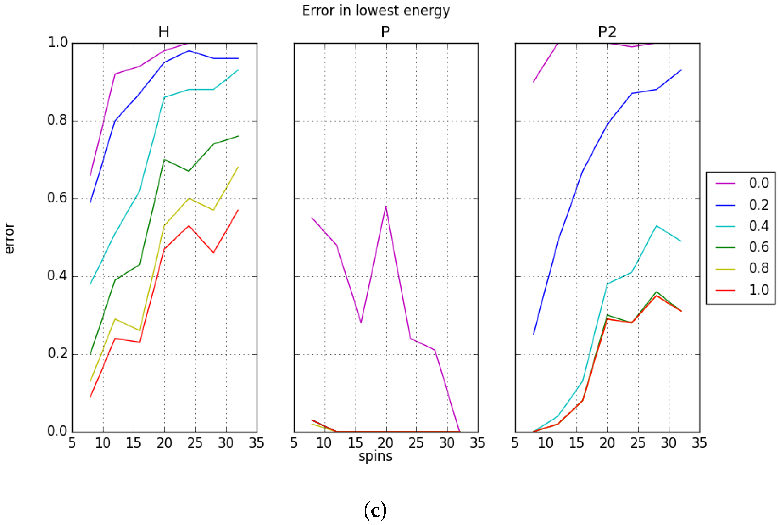
We define the error in recall as the number of instances where the sought memory is not the lowest energy state for the system. Instead, the lowest energy state for the system may correspond to a spurious state or any other state that arises from overlap in the memories. The measured recall errors with random memories are shown in
Figure 5. We note that the low error for the low capacity case agrees with the high recall accuracy in
Figure 4a. The recall error is more substantial for the higher capacity cases, but this does not always explain the loss in recall accuracy. For example, the behavior of the projection rule
P shown in
Figure 4b can be compared to the recall error presented in
Figure 5b. It is apparent from this comparison that the loss in recall accuracy does not arise from returning a lower energy state, but rather from returning a higher energy state. By contrast, for both
H and
, as the capacity and system sizes increase, the error increases even with bias applied. This is not the typical case for
P; there is only one instance where the error is above 0 in the presence of bias. We conclude that at larger system sizes,
P is not finding its lowest energy. Currently, no explanation for this behavior is known.
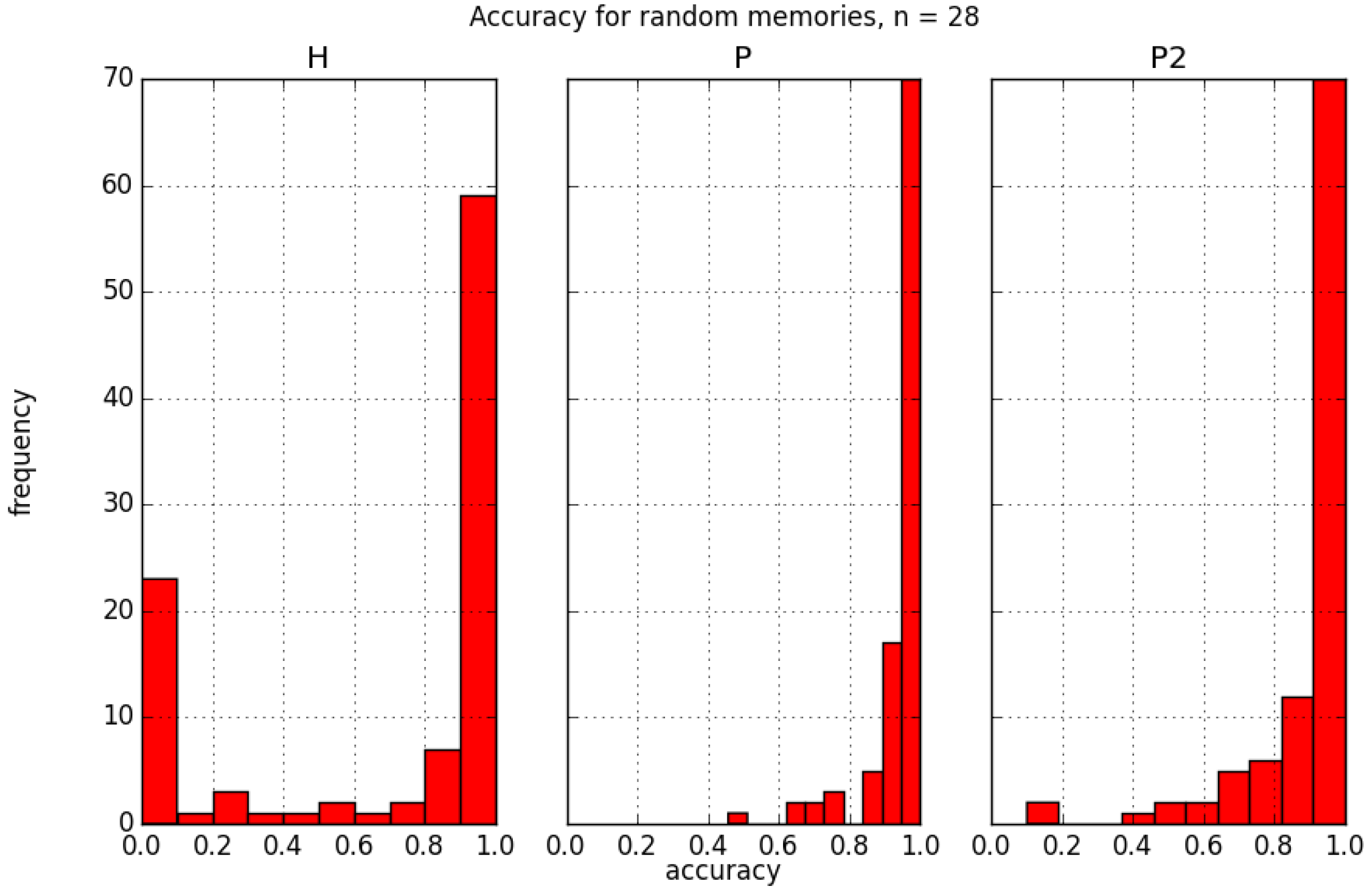
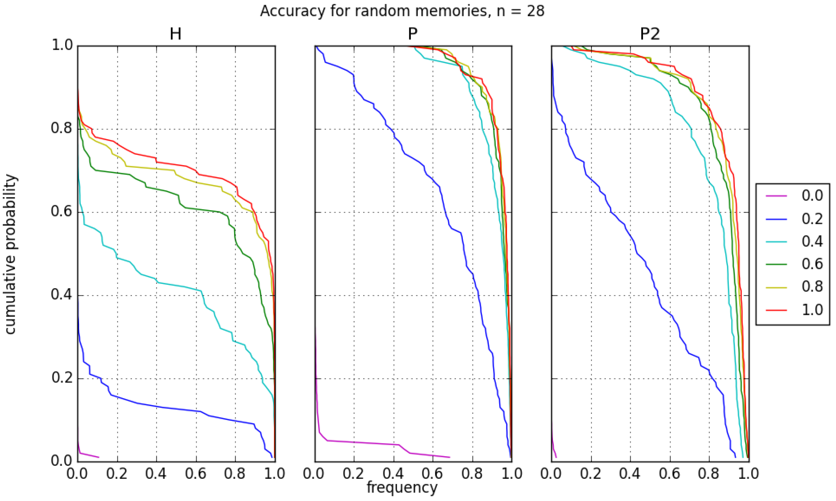
The reported recall accuracy is the average of recall success for an ensemble of 100 problems. The distribution of these successes is shown in
Figure 6, with each panel corresponding to a different learning rule. For each plot, the size of the system is
, the number of stored memories is
, and the applied bias is
. The histograms show the frequency with which different probabilities of success are observed. It is notable that the distributions are not the same for each learning rule and, in particular, the Hebb rule demonstrate a bimodal distribution not seen in the projection rule. Though
H has a high frequency around
, it also has a significant frequency around
. The
P and
rules have high frequency around
with decreasing frequencies for lower accuracies. These histograms can be used to create cumulative distribution plots for the recall accuracy. Such a plot can be used to indicate the probability of achieving a desired recall accuracy or better,
. For instance, in
Figure 7 with
P and bias of
,
. The probability of achieving recall accuracy of greater than
is about
. This provides a means to determine how many iterations on the D-Wave would be needed to achieve a desired accuracy within a given tolerance.
Of additional interest is the comparison of the projection rules P and , for which the weight matrix decorrelates memories. Both rules generally perform better than the Hebb rule, however, we see that outperforms recall P in instances with higher capacity or larger system sizes. The primary distinction between P and is the complete versus bipartite graph structure for storing the weight patterns. Both rules require the same number of logical qubits, but requires fewer physical qubits due to its smaller edge set. However, as shown in the distribution of recall accuracy, the rules have a broad distribution of error for these relatively small sample sizes. Though its contribution is not as drastic as memory size and learning rule, the applied bias also clearly affects the recall accuracy. For H, the bias trends are somewhat spaced out and follow similar paths. For P and , the bias lines for bias above are much closer together. As expected, a higher bias improves the recall accuracy though the gain is not generally significant in P and . It has greater influence for H.

