Statistics of Binary Exchange of Energy or Money

Abstract

Why does the Maxwell-Boltzmann energy distribution for an ideal classical gas have an exponentially thin tail at high energies, while the Kaniadakis distribution for a relativistic gas has a power-law fat tail? We argue that a crucial role is played by the kinematics of the binary collisions. In the classical case the probability of an energy exchange far from the average (i.e., close to 0% or 100%) is quite large, while in the extreme relativistic case it is small. We compare these properties with the concept of “saving propensity”, employed in econophysics to define the fraction of their money that individuals put at stake in economic interactions.

1. Introduction

In this work, we study with statistical methods a problem concerning the elastic scattering of two particles in the relativistic regime and we discuss the similarities between this physical process and the economic interactions occurring in the so-called wealth exchange models [1,2]. A unifying element in this analysis is the generalized $\kappa$-distribution [3,4,5,6], which has proven to be helpful for the description of both kinds of phenomena. We start from the familiar assumption of statistical mechanics according to which the macroscopic distributions (of energy or income) are determined by the microscopic interactions (between molecules or, respectively, individuals). Such interactions can be of many different sorts, but we are mostly interested into properties which are independent from the details of the specific system; namely we are interested into the conditions under which a “fat” power-law tail can appear in the macroscopic distribution, instead of the thin exponential tail typical of the Boltzmann distribution.

In our computation we shall suppose that all the permitted final states of a binary collision (those compatible with conservation laws) have the same probability. For this reason we mention in the title the “statistics of binary exchange”, and not the dynamics of this exchange. “Statistics” is meant here in the same sense as in the term “Statistical Mechanics”. In fact, it is known from experimental data on relativistic gases and cosmic rays that the fat tails in their energy distributions have some universal features; it is also known that Pareto tails in income distributions have existed in various epochs and in countries with very different economic systems. (For some very recent data and related analysis see [7].) This suggests that the formation mechanism of the tails is essentially kinematical. In [3] G. Kaniadakis has shown that the deformation of the distribution function introduced by the parameter $\kappa$ emerges naturally within Einstein’s special relativity, so that one can see the $\kappa$-deformation as a pure relativistic effect. To this end, one first proves that the $\kappa$-deformed sum of the momenta of two particles is the additivity law for the relativistic momenta (the $\kappa$-sum is used in a generalized entropy minimization procedure leading to the $\kappa$-distribution). By considering, in the framework of special relativity, the $\kappa$-statistics of an ensemble of identical particles, one therefore arrives at a distribution with a power-law tail without any assumption on dynamics, but using only kinematics.

From the physical point of view, what are the main differences between a “classical” collision and a strongly relativistic collision? The answer is not unique. The techniques of relativistic kinetic theory [8] allow us to write the Boltzmann equation in relativistic form and to conduct a similar analysis as done in the classical theory. Nevertheless, the approach by Kaniadakis et al. shows that there is still room for a better understanding of the basic concepts. In our opinion, it is important to consider also quantities that are not Lorentz-invariant, and are therefore often disregarded in the traditional relativistic kinetic theory. We will focus our attention on the non-invariant fraction R of energy which is transferred from one particle to the other during a binary collision between identical particles. If one looks at the collision in the center of mass system, R is trivially zero, because the conservation laws of the total energy and momentum impose that the energy is equally distributed between the two particles before and after the scattering. What changes in the collision, as seen from the center of mass system, is only the direction of the momenta. Any other change is entirely due to the choice of a different reference system.

Nevertheless, for a gas contained in a finite volume there exists a privileged reference system, namely the system where the gas is, on average, at rest. If we look at a scattering process as the analogue of an economic interaction, the fraction R of money exchanged by an individual is obviously an important quantity. We point out that in any realistic income distribution the majority of the individuals have low or middle income, therefore it is important to evaluate R for an interaction between a poor individual (slow molecule) and a rich one (fast molecule). It has been suggested by some authors [9] that Pareto tails are formed when the rich part of a population enacts an effective policy for preserving its wealth in the interactions. This attitude can also be described as a high “saving propensity”. In [10] we have argued that something similar happens in relativistic collisions, but the technique employed did not allow us to carry the analogy very far. In this work we improve the technique for the calculation of the R factor and we obtain further results. In Section 2 we evaluate the probability distribution of energy transfer in an elastic collision. We solve numerically the conservation law for energy and compute the integral over final states parametrized as a one-parameter line in phase space. In Section 3 we give the results of agent-based simulations based on money exchange rules which are the analogues of the energy balance in the collisions. Section 4 comprises our conclusions. The Appendices contain some background material on relativistic energy and momentum (Appendix A) and wealth exchange models in econophysics (Appendix B) that can be helpful for an interdisciplinary audience.

The question raised at the beginning of the abstract of this paper is therefore answered in two steps. In the first step (Section 2) we show that the probability of final states of a binary collision is different in the case of a low-energy and high-energy collision. In the second step (Section 3) we pass “from micro to macro” by simulating a large number of collisions occurring with this probability, and we look at what kind of equilibrium distribution they lead to in a large population of molecules.

2. Energy Transfer in an Elastic Collision

2.1. General Expression

In this Section we consider the relativistic scattering of two identical particles of mass m and compute the probability distribution of the fraction R of kinetic energy transferred in the collision, supposing that all final states are equally probable. The incoming particle is labelled as “Particle 1” and the other, which is initially at rest, as “Particle 2”. The initial velocity of Particle 1 is directed along x and is denoted simply as v. The reference system can be chosen in such a way that the final momenta of the particles have components only along x and y, denoted as $p_{1x}$, $p_{1y}$, $p_{2x}$, $p_{2y}$. Momentum conservation in the directions x and y imposes that

$$\begin{array}{c}{p}_{2y}=-p_{1y};\hfill \end{array}$$

(1)

$$\begin{array}{c}{p}_{2x}=p-p_{1x},\hfill \end{array}$$

(2)

where p is the initial momentum of Particle 1: $p=mv/\sqrt{1-v^2/c^2}=mv\gamma$. In the following we use units such that $c=1$. Energy conservation requires that

$$\begin{array}{c}\hfill E=E_1+E_2=\sqrt{m^2+p_{1x}^2+p_{1y}^2}+\sqrt{m^2+p_{2x}^2+p_{2y}^2},\end{array}$$

(3)

where E is the total energy $E=\sqrt{m^2+p^2}$ and $E_1$ and $E_2$ are the energies of the particles after the collision. The collision is supposed to be elastic. The fraction R of the initial kinetic energy of Particle 1 which is transferred to Particle 2 after the collision is

$$\begin{array}{c}\hfill R=\frac{E_2-m}{E-m}=\frac{\sqrt{m^2+p_{2x}^2+p_{2y}^2}-m}{\sqrt{m^2+p^2}-m}\end{array}$$

(4)

The conservation laws (1)–(3), taken together, make up a system with 4 unknowns and 3 equations, which has infinite solutions dependent on one parameter, say t. It is convenient to choose as parameter $p_{1x}$, the final momentum of Particle 1 along x. The value of this momentum spans a finite interval, because the minimum it can take is 0 (when the full momentum of the incoming particle is transferred to Particle 2, like in a frontal billiard scattering), and the maximum is p (when there is no momentum transfer at all). In the four-dimensional Euclidean vector space of the final momenta of the two particles ($p_{1x}$, $p_{1y}$, $p_{2x}$, $p_{2y}$), the one-parameter subset of the solutions of Equations (1)–(3) can be written as

$$\left\{\begin{array}{ccc}{p}_{1x}& =& t\hfill \\ p_{1y}& =& g\left(t\right)\hfill \\ p_{2x}& =& h\left(t\right)=p-t\hfill \\ p_{2y}& =& -g\left(t\right)\hfill \end{array}\right.,$$

(5)

where $t\in [0,p]$ and $g\left(t\right)$ is the solution of Equation (3), which is now rewritten as

$$\sqrt{m^2+p^2}=\sqrt{m^2+t^2+{\left[g\left(t\right)\right]}^2}+\sqrt{m^2+{(p-t)}^2+{[-g\left(t\right)]}^2}.$$

(6)

The subset (5) is a path whose invariant length is given by

$$L={\int }_0^p\sqrt{1+{\left[g^{\prime }\left(t\right)\right]}^2+{\left[h^{\prime }\left(t\right)\right]}^2+{[-g^{\prime }\left(t\right)]}^2}dt.$$

(7)

In order to evaluate the average value in the final state of any quantity F depending on $p_{1x}$, $p_{1y}$, $p_{2x}$, $p_{2y}$, according to the ensemble averaging procedure familiar from statistical mechanics, we must compute the weighted integral

$$⟨F⟩=\frac{\int d{p}_{1x}\int d{p}_{2x}\int d{p}_{1y}\int d{p}_{2y}P(p_{1x},p_{1y},p_{2x},p_{2y})F(p_{1x},p_{1y},p_{2x},p_{2y})}{\int d{p}_{1x}\int d{p}_{2x}\int d{p}_{1y}\int d{p}_{2y}P(p_{1x},p_{1y},p_{2x},p_{2y})},$$

(8)

where P is the appropriate probability density distribution. In this case, since we suppose that all possible final states of the scattering process are equiprobable, the function P is a constant function with support along the path (5). Therefore the four-dimensional integrals reduce to line integrals and we obtain

$$⟨F⟩=\frac{1}{L}{\int }_0^p\sqrt{1+{\left[g^{\prime }\left(t\right)\right]}^2+{\left[h^{\prime }\left(t\right)\right]}^2+{[-g^{\prime }\left(t\right)]}^2}Fdt,$$

(9)

where F is evaluated, through the momenta, as a function of t:

$$F\to F\left[p_{1x}\left(t\right),p_{1y}\left(t\right),p_{2x}\left(t\right),p_{2y}\left(t\right)\right].$$

(10)

In particular, we shall take as F the energy ratio R defined in (4). Note that L and $⟨F⟩$ do not depend on the choice of the parameter t. The factor which multiplies F in the integral (9) is the parameter-invariant infinitesimal length $ds$ of the path. This implements the physical intuition that any infinitesimal invariant interval of possible final states with the same length $ds$ has the same probability.

Note that Equation (4) can be seen as interpolating between the purely non-relativistic case for which R is given by ${\mathbf{p}}_2^2/p^2$, and the purely massless relativistic case for which R depends on the square root of the non-relativistic ratio. This transition in the effective functional dependence of R on ${\mathbf{p}}_2^2$ and $p^2$ (as compared with the classical case) reflects the role of mass as a form of “savings” in the relativistic mass shell constraint. (We thank an anonymous referee for this remark.)

2.2. Numerical Solution of the Conservation Laws

Our strategy is to use the conservation laws (1)–(3) to express the final momenta $p_{1y}$, $p_{2x}$, $p_{2y}$ as functions of $p_{1x}$. So $p_{1x}$ becomes our integration parameter t. However, the energy conservation relation (3) cannot be solved analytically. We thus transform it into a first-order differential equation by taking the total differential of Equation (3), which gives

$$0=\left(\frac{\partial E_1}{\partial p_{1x}}-\frac{\partial E_2}{\partial p_{2x}}\right)d{p}_{1x}+\left(\frac{\partial E_1}{\partial p_{1y}}-\frac{\partial E_2}{\partial p_{2y}}\right)d{p}_{1y}.$$

(11)

From this, with some straightforward algebraic steps, we obtain

$$\frac{d{p}_{1y}}{d{p}_{1x}}=-\frac{1}{p_{1y}E}\left[p_{1x}\sqrt{m^2+{(p-p_{1x})}^2+p_{1y}^2}-(p-p_{1x})\sqrt{m^2+p_{1x}^2+p_{1y}^2}\right].$$

(12)

With the notation introduced in Equation (5) this can be rewritten in a form which is mathematically more transparent, recalling that m and p are fixed constants:

$$g^{\prime }\left(t\right)=-\frac{1}{g\left(t\right)\sqrt{m^2+p^2}}\left[t\sqrt{m^2+{(p-t)}^2+g^2\left(t\right)}-(p-t)\sqrt{m^2+t^2+g^2\left(t\right)}\right].$$

(13)

In the following, however, we shall denote the parameter t by $p_{1x}$, according to its physical meaning.

We are interested into the numerical solution of this equation via a Runge-Kutta algorithm in the interval $p_{1x}\in [0,p]$. It can be shown that the right hand sidediverges when $p_{1x}\to 0^{+}$ or $p_{1x}\to p^{-}$, so it is impossible to use the points $p_{1x}=0$ or $p_{1x}=p$ to set the the initial conditions of the numerical integration. It is possible, however, to impose the initial conditions at the value of $p_{1x}$ which solves Equation (3) in the special case $p_{1x}=p_{1y}=\xi$. In this case Equation (3) or its equivalent (6) become

$$\sqrt{m^2+p^2}=\sqrt{m^2+2{\xi }^2}+\sqrt{m^2+{(p-\xi )}^2+{\xi }^2}$$

(14)

and can be solved numerically, thus finding appropriate initial conditions for the differential equation. The solution of the latter can then be extended on the whole interval $[0,p]$ by considering that: (1) The solution is symmetric with respect to $p/2$. (2) The solution in the restricted interval $[\epsilon ,p-\epsilon ]$ converges when $\epsilon \to 0$. (One obtains numerical evidence of this property using small values of $\epsilon$; the convergence follows from the fact that for any fixed $\epsilon$ the derivative $g^{\prime }$ behaves as $1/{\epsilon }^{\alpha }$, with $0<\alpha <1$, when $p_{1x}=\epsilon$ or $p_{1x}=p-\epsilon$.)

An example of the solution, which we shall denote as $g\left(p_{1x}\right)$, is given in Figure 1.

Figure 1. The function $g\left(p_{1x}\right)$ obtained by numerical solution of the differential Equation (12), for a strongly relativistic case ($p/m=\gamma v=100\simeq \gamma$; $v\simeq 1$). We use units $c=1$ throughout the paper, and in this plot we also take $m=1$ for graphical reasons.

2.3. Monte Carlo Evaluation of the Integral on Final States

The line integral (9) can be now computed through a Monte Carlo technique, since we have a numerical relation between $p_{1x}$ and $p_{1y}$, while $p_{2x}$ and $p_{2y}$ can be obtained through the momentum conservation laws (1) and (2). For any function F of the final momenta, the average value $⟨F⟩$ will only depend on the initial momentum p. We can therefore study the dependence of $⟨F⟩$ on p distinguishing between the classical limit ($\gamma \to 1^{+}$, $v\ll 1$ in our units) and the strongly relativistic limit ($\gamma \gg 1$, $v\to 1^{-}$). If we take $F=R$, it turns out that $⟨R⟩$ is actually independent from p and is always equal to $1/2$. This is due to the symmetry of the function $g\left(p_{1x}\right)$ (compare Figure 1). It is more interesting to consider the probability distribution of R in the interval $I_1=\{p_{1x}\in [p/2,p]\}$. This corresponds to collisions in which Particle 2 has obtained from Particle 1 a kinetic energy between 0 and $1/2$ of its initial kinetic energy (the values 0 and $1/2$ being respectively obtained when $p_{1x}=p$ and $p_{1x}=p/2$). The complementary interval in the possible final states, namely $I_2=\{p_{1x}\in [0,p/2]\}$, represents the complementary cases of energy re-distribution, but since the two particles are identical, those cases are not distinguishable from the corresponding cases in $I_1$, as far as their effect on the income distribution is concerned.

Let us make a numerical example with reference to Figure 2, which represents the probability distribution of R in a collision with low energy; then we shall compare this to the distribution in the extreme-relativistic case. The distribution in Figure 2 is obtained as follows:

Figure 2. Plot of the distribution of R in a Monte Carlo simulation of $5\times {10}^6$ almost classical collisions ($p/m=\gamma v=0.01$, $\gamma \simeq 1$, $v\simeq {10}^{-2}$). R is expressed in % and is the fraction of kinetic energy transferred from Particle 1 to Particle 2. When $p/m$ becomes even smaller, in the fully classical case, the peak for $R\to 0$ (corresponding to a symmetric peak for $R\to 1$) becomes higher. The dot at $R=51\%$ is not meaningful.

• A numerical value of $p/m$ is chosen, in this example $p/m=0.01$, and Equation (12) is solved numerically, obtaining $p_{1y}$ as a function g of $p_{1x}$: $p_{1y}=g\left(p_{1x}\right)$.
• A large number of random values of $p_{1x}$ (typically ${10}^6$ or ${10}^7$) is generated in the interval $I_1$.
• The corresponding value of R is calculated from the definition (4) using the function $g\left(p_{1x}\right)$ and Equations (1) and (2).
• Each value of R is multiplied by the weight $\sqrt{{(p_{1x}^{\prime })}^2+{(p_{1y}^{\prime })}^2+{(p_{2x}^{\prime })}^2+{(p_{2y}^{\prime })}^2}$.
• In the graph, which is actually a histogram, the vertical axis represents, for 50 discretized values of R in the interval $0\le R\le 1/2$, the weighted number of counts, i.e., the number of times R has taken that value, multiplied by the weight. The part of the histogram for $1/2\le R<1$ is symmetrical, and not shown.

For instance, in the almost-classical case of Figure 2 ($p/m=0.01$), the probability that $R=0.4=40\%$, i.e., Particle 1 has lost to Particle 2 the 40% of its initial kinetic energy, is approximately $1/3$ of the probability that $R=0.05=5\%$. Note that the probability of $R=60\%$ is equal to the probability of $R=40\%$ and in both cases the collision will have the same effective result, with one of the particles having 60% of the initial energy and the other 40%.

On the other hand, in the extreme relativistic case (Figure 3) the probability of R turns out to be almost independent from R. In other words, there will not be a majority of collisions with very small or very large energy exchange like in Figure 2, but each rate of energy redistribution has approximately the same probability. This marks a clear difference between low energy and high energy regimes. In Section 3 we shall use an agent-based simulation to see how this affects the equilibrium distribution in an analogous economic system.

Figure 3. Plot of the distribution of R in a Monte Carlo simulation of $5\times {10}^6$ collisions, in a fully relativistic case ($p/m=\gamma v=1000\simeq \gamma$, $v\simeq 1$). R is expressed in % and is the fraction of kinetic energy transferred from Particle 1 to Particle 2. The dot at $R=51\%$ is not meaningful.

3. Agent-Based Simulations and Saving Propensity

The analogies between the energy distribution in a gas and the income distribution in a society have been one of the main subjects of econophysics, since the pioneering works of the 1990s [9]. In several works, agent-based simulations have been employed to investigate the relation between the rules of the microscopic interactions and the resulting equilibrium income distribution. A well established result is that a fixed saving propensity in the interactions gives rise to a distribution of the Gamma-kind, namely $P\left(E\right)=k{E}^{\beta }{e}^{-E/T}$, where E is here the income and T an effective temperature. This distribution does not have a flat tail. ($P\left(E\right)$ is the probability density distribution of energy or money, in the econophysics analogy. The probability that an individual chosen at random has income in the infinitesimal interval $(E,E+dE)$ is given by $P\left(E\right)dE$. The “temperature” T corresponds essentially, in the analogy, to the average wealth, whereby the Boltzmann constant is set by convention equal to 1.)

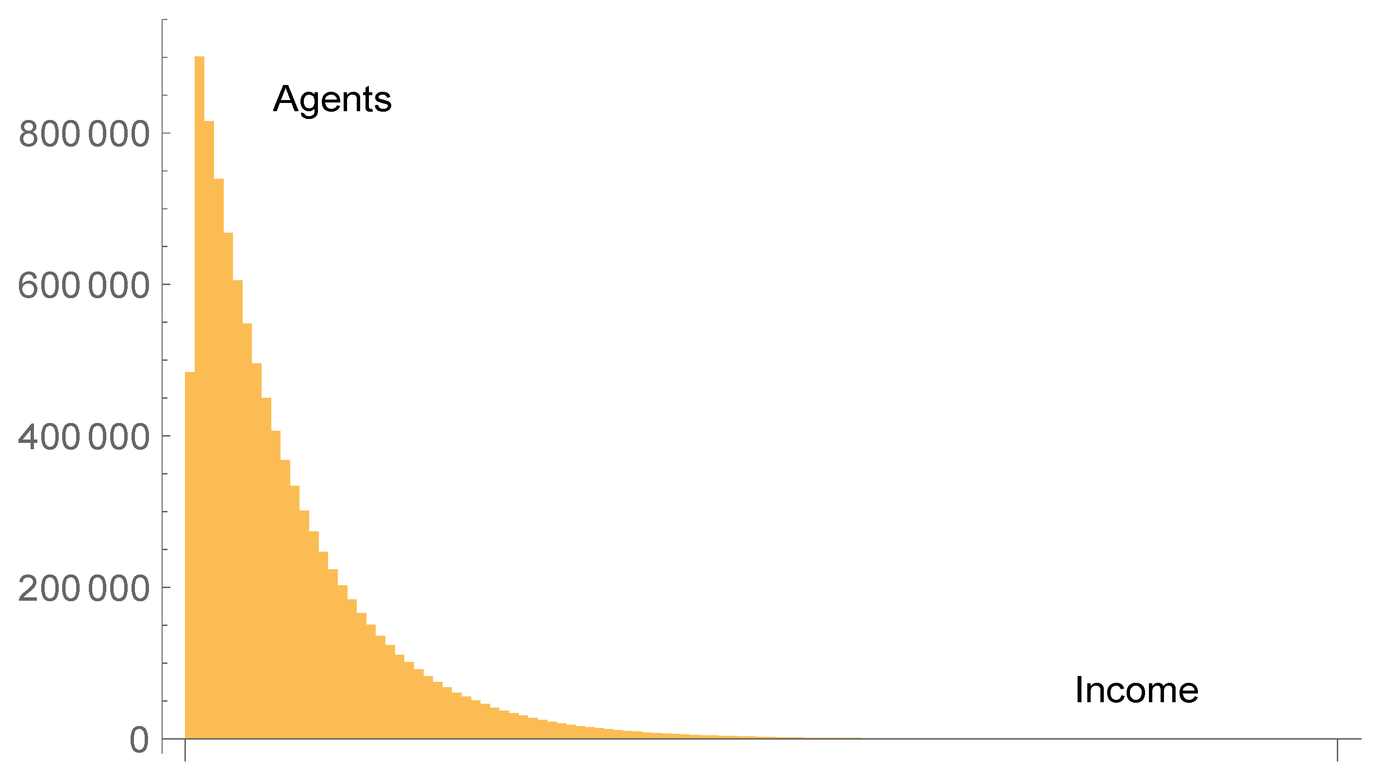
The saving propensity, usually denoted with $\lambda$, is the fraction of its income that each individual “hedges” in the economic interactions, or in other words, individuals put at stake in the interactions a fraction $(1-\lambda )$ of their income. It is relatively straightforward to reproduce some of the mentioned result. For instance, Figure 4 shows the income distribution we have obtained from a simulation with ${10}^5$ agents exchanging energy/money according to the rule [11]

$$\begin{array}{c}{E}_i^{\prime }=\lambda E_i+\xi (1-\lambda )(E_i+E_j),\hfill \\ E_j^{\prime }=\lambda E_j+(1-\xi )(1-\lambda )(E_i+E_j)\hfill \end{array}$$

(15)

(i and j label two agents randomly chosen at each step; $\xi$ is a random variable in the interval $(0,1)$). The system has been evolved to equilibrium with a series of ${10}^8$ binary exchanges, and the whole procedure averaged for 50 times in order to minimize the effect of fluctuations.

Figure 4. Income distribution from an agent-based simulation (see details in text) where agents exchange money with a fixed saving propensity. A fit with the $\kappa$-distribution confirms that there is no Pareto tail.

More in detail, we define, in a suitable programming language (Mathematica in our case) a vector $\mathbf{E}$ with ${10}^5$ components. The component $E_i$ represents the wealth of the i-th agent of our idealized society. At the beginning all agents have the same wealth, e.g., $E_i=20$ units for any i in our simulation. Then the simulation algorithm choses at random two integer indices i, j between 1 and ${10}^5$. These are the agents who are currently interacting. Their wealths are changed according to Equation (15). The random choice of agents and the modification of their wealths is repeated for ${10}^8$ times. This means that, on average, each agent has interacted with others for ${10}^3$ times. (Thermalization times larger than ${10}^8$ steps are found to give no changes in the final results.) A histogram of the wealth distribution is generated by rounding the wealth of each agent to the nearest integer and then using a counting function to define the frequency, for instance in Mathematica in our case with the code frequency = Table[Count[X,n],{n,0,120}], where X is the rounded income vector and 120 is a safe maximum value for the income. The frequency vector is the one whose components are shown in the histograms in Figure 4 and Figure 5. Next we average the frequency vector over many realizations, in order to reduce the fluctuations, we normalize it by dividing each component by the sum of all components, and we use a FindFit function to fit it to the $\kappa$-distribution (16). This function employs a least-squares method and returns the best fit values of the three parameters in the $\kappa$-distribution. When the fit fails to show a power-law tail, it is because it returns negative values for $\alpha$ and $\beta$, which are not admissible for a $\kappa$-distribution.

Figure 5. Income distribution from an agent-based simulation (see details in text) with agents which exchange money in analogy with the behavior of relativistic particles, i.e., all exchange rates being equiprobable. The distribution has a Pareto tail proportional to $1/E^{2.75}$, where E is the income.

A fit of the resulting distribution with the $\kappa$-distribution

$$P\left(E\right)=\frac{\alpha \beta E^{\alpha -1}{exp}_{\kappa }(-\beta E^{\alpha })}{\sqrt{1+{\beta }^2{\kappa }^2{E}^{2\alpha }}};$$

(16)

$${exp}_{\kappa }\left(t\right)={\left(\sqrt{1+{\kappa }^2{t}^2}+\kappa t\right)}^{1/\kappa }$$

(17)

fails, and this confirms that no Pareto tail is present. Similar results can be obtained with other values of $\lambda$.

Now let us run a simulation with microscopic exchange rules corresponding to the extreme relativistic case of Section 2.3. We set the energies of two particles after a collision as

$$\begin{array}{c}{E}_i^{\prime }=\xi (E_i+E_j),\hfill \\ E_j^{\prime }=(1-\xi )(E_i+E_j)\hfill \end{array}$$

(18)

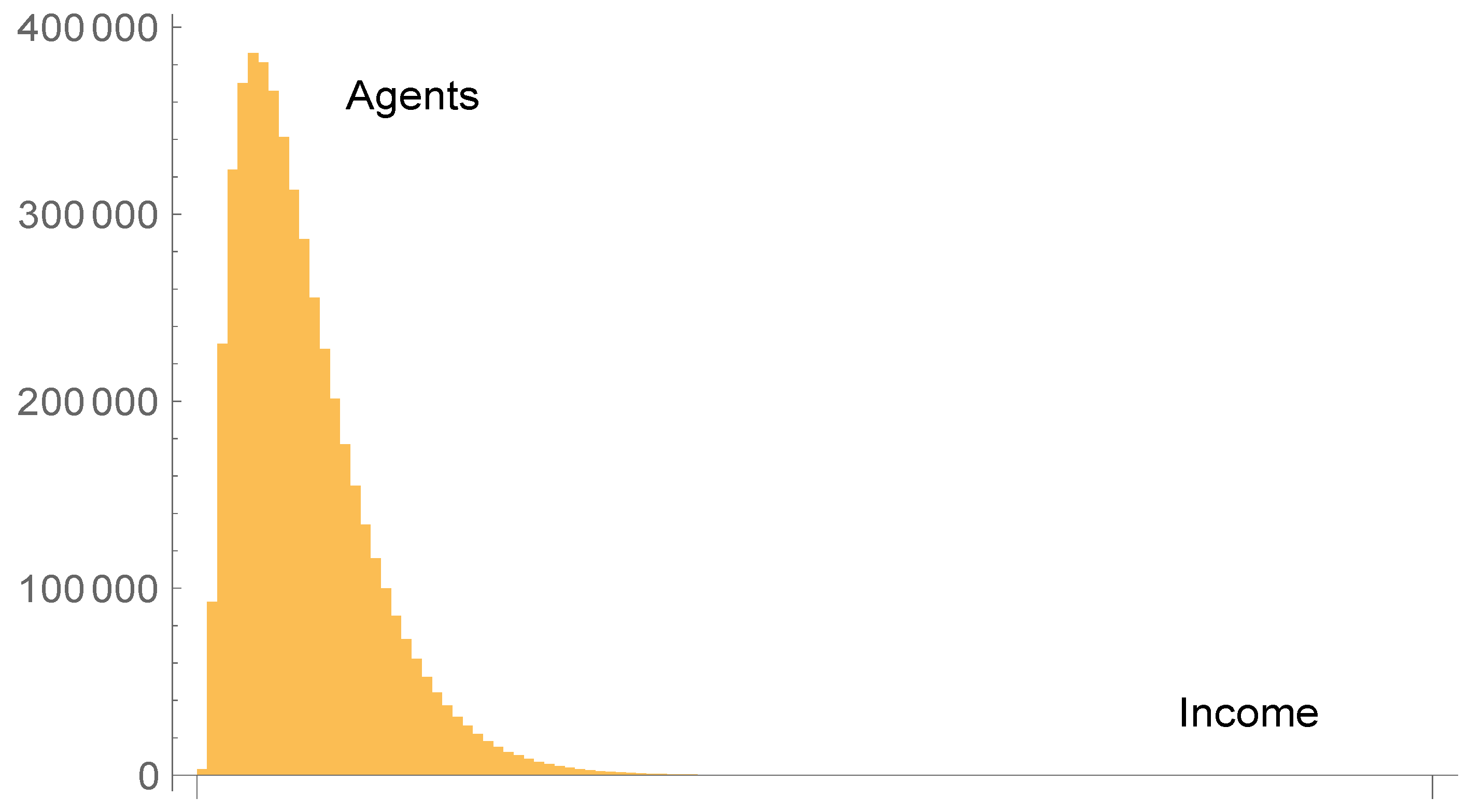
This means that, as found in Section 2.3, all energy exchange rates are equally probable, and as a consequence there is no fixed saving propensity. The result of a simulation with ${10}^5$ agents, ${10}^8$ thermalization steps and 100 averages is given in Figure 5. The curve can be fitted by a $\kappa$-distribution with a ratio $\alpha /\kappa \simeq 1.75$, thus with a Pareto tail of exponent 2.75.

4. Conclusions

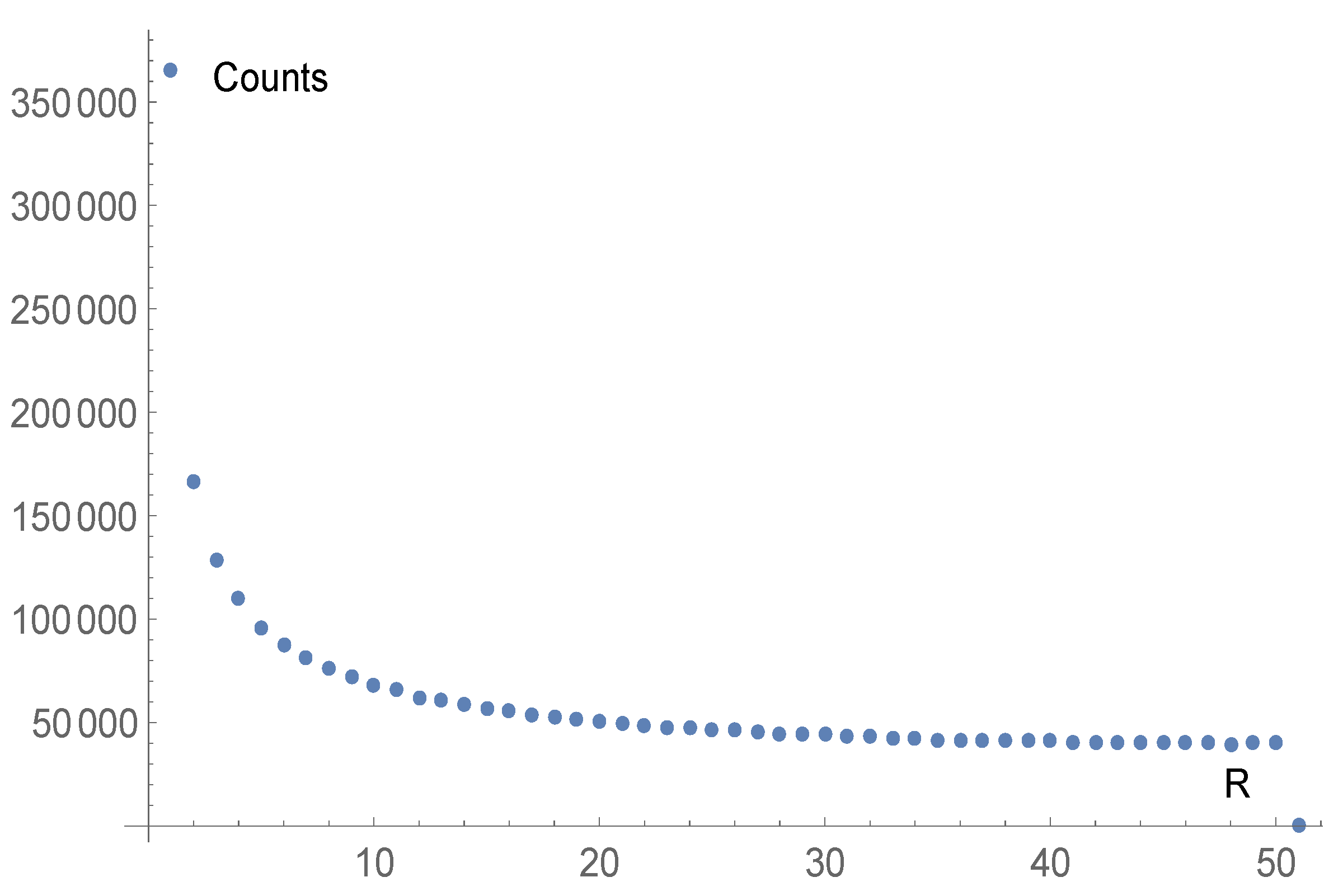
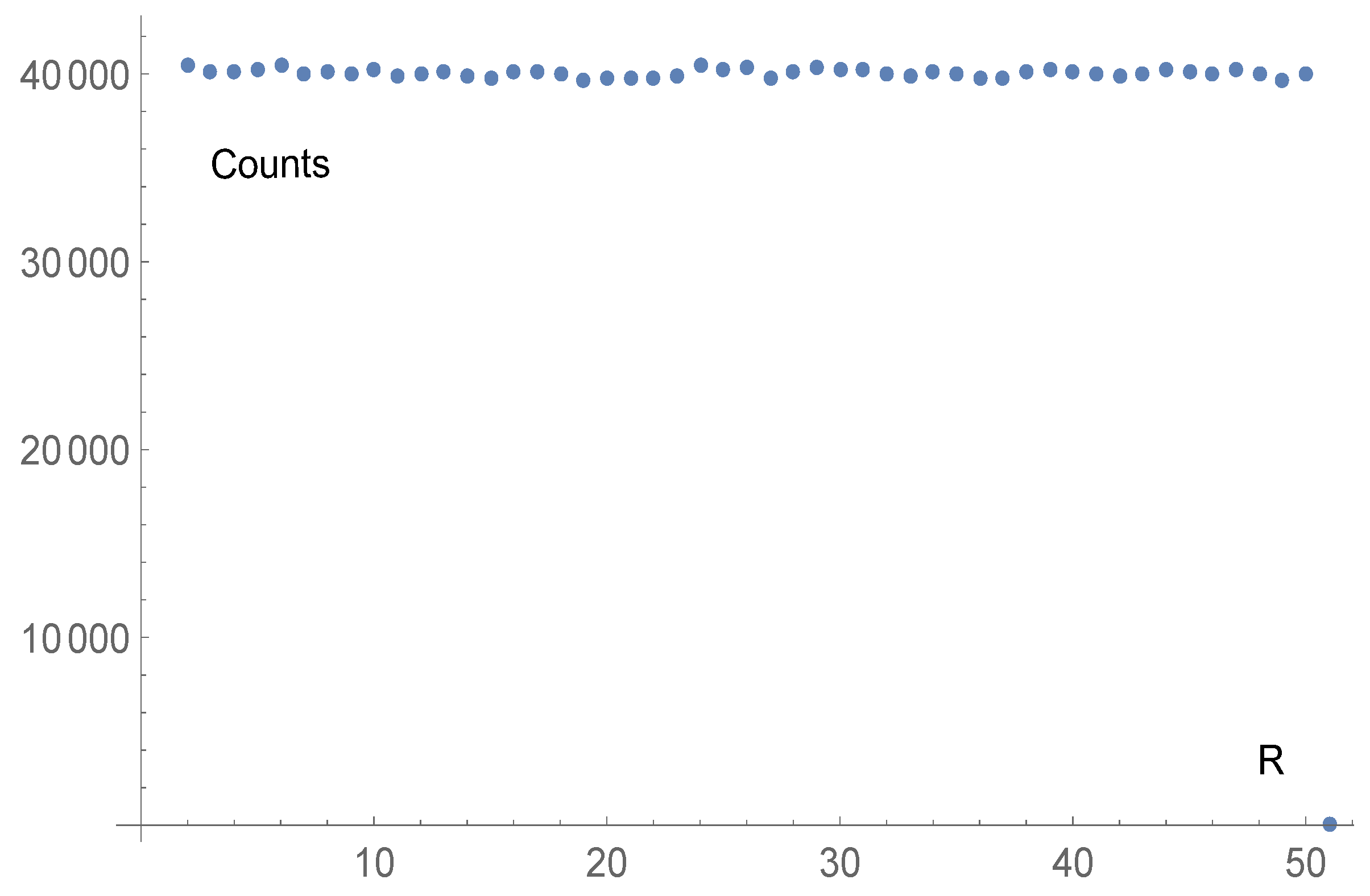
Pursuing an analogy between physics and economics, we have computed the probability that in a relativistic collision between two identical particles the fraction R of energy exchanged is equal to a given value in the interval $(0,1)$, thus obtaining a distribution for R. This is accomplished under the assumption that all the possible final states of the collision are equiprobable, i.e., considering only kinematical constraints. The evaluation is done in the reference system where one of the particles is at rest; this choice is motivated by an economic analogy and by the fact that the privileged reference frame for a gas is the frame where most molecules have velocity close to zero.

We have represented the possible final states as a one-parameter line in the 4D space of the final momenta. A Monte Carlo algorithm then generates states uniformly distributed along this line, weighted by the invariant length element of the line. This allows us to obtain a histogram of the values of R. In the non-relativistic limit the histogram has a sharp peak for $R\to 0^{+}$ (and symmetrically for $R\to 1^{-}$). By contrast, in the relativistic case, when the incoming particle has a large $\gamma$ factor, the histogram is essentially flat. This means that, from the kinematical point of view, in strongly relativistic collisions particles can easily exchange any fraction of their total energy.

The analogue of a relativistic collision in economic interactions is therefore a money exchange without a fixed saving propensity. We have checked through agent-based simulations that interactions of this kind lead to an income distribution with a Pareto tail. This confirms and extends the results of [10], albeit with the limitation inherent to the analogy employed and to the specific physical process and reference frame considered. Moreover, the present results hold for collisions between identical particles, while in [10] the particles were considered to be distinguishable.

References

- Gallegati, M.; Kirman, A. Reconstructing economics: Agent based models and complexity. Complex. Econ. 2012, 1, 5–31. [Google Scholar] [CrossRef]
- Tesfatsion, L. Agent-based computational economics: Modeling economies as complex adaptive systems. Inf. Sci. 2003, 149, 263–269. [Google Scholar] [CrossRef]
- Kaniadakis, G. Statistical mechanics in the context of special relativity. Phys. Rev. E 2002, 66. [Google Scholar] [CrossRef] [PubMed]
- Kaniadakis, G. Theoretical foundations and mathematical formalism of the power-law tailed statistical distributions. Entropy 2013, 15, 3983–4010. [Google Scholar] [CrossRef]
- Trivellato, B. Deformed exponentials and applications to finance. Entropy 2013, 15, 3471–3489. [Google Scholar] [CrossRef]
- Scarfone, A.M. Entropic forms and related algebras. Entropy 2013, 15, 624–649. [Google Scholar] [CrossRef]
- Xu, Y.; Wang, Y.; Tao, X.; Ližbetinová, L. Evidence of Chinese income dynamics and its effects on income scaling law. Phys. A Stat. Mech. Its Appl. 2017, 487, 143–152. [Google Scholar] [CrossRef]
- De Groot, S.R. Relativistic Kinetic Theory: Principles and Applications; Elsevier: Amsterdam, The Nertherlands, 1980. [Google Scholar]
- Yakovenko, V.M.; Barkley Rosser, J. Colloquium: Statistical mechanics of money, wealth, and income. Rev. Mod. Phys. 2009, 81. [Google Scholar] [CrossRef]
- Modanese, G. Common origin of power-law tails in income distributions and relativistic gases. Phys. Lett. A 2016, 380, 29–32. [Google Scholar] [CrossRef]
- Chakraborti, A.; Chakrabarti, B.K. Statistical mechanics of money: How saving propensity affects its distribution. Eur. Phys. J. B 2000, 17, 167–170. [Google Scholar] [CrossRef]
- Ispolatov, S.; Krapivsky, P.L.; Redner, S. Wealth distributions in asset exchange models. Eur. Phys. J. B 1998, 2, 267–276. [Google Scholar] [CrossRef]
- Mantegna, R.N.; Stanley, H.E. An Introduction to Econophysics; Cambridge University Press: Cambridge, UK, 2000. [Google Scholar]
- Schinckus, C. Between complexity of modelling and modelling of complexity: An essay on econophysics. Phys. A Stat. Mech. Its Appl. 2013, 392, 3654–3665. [Google Scholar] [CrossRef]
- Bertotti, M.L.; Modanese, G. Discretized kinetic theory on scale-free networks. Eur. Phys. J. Spec. Top. 2016, 225, 1879–1891. [Google Scholar] [CrossRef]
- Di Matteo, T.; Aste, T.; Hyde, S.T. Exchanges in complex networks: Income and wealth distributions. In The Physics of Complex Systems (New Advances and Perspectives); Mallamace, F., Stanley, H.E., Eds.; IOS Press: Amsterdam, The Netherlands, 2003; p. 435. [Google Scholar]
- Boghosian, B.M. Kinetics of wealth and the Pareto law. Phys. Rev. E 2014, 89. [Google Scholar] [CrossRef] [PubMed]
- Boghosian, B.M.; Johnson, M.; Marcq, J.A. An H theorem for Boltzmann’s equation for the Yard-Sale Model of asset exchange. J. Stat. Phys. 2015, 161, 1339–1350. [Google Scholar] [CrossRef]
- Boghosian, B.M. Fokker-Planck description of wealth dynamics and the origin of Pareto’s law. Int. J. Mod. Phy. C 2014, 25. [Google Scholar] [CrossRef]
- Challet, D.; Marsili, M.; Zecchina, R. Statistical mechanics of systems with heterogeneous agents: Minority games. Phys. Rev. Lett. 2000, 84, 1824–1827. [Google Scholar] [CrossRef] [PubMed]
- Vallejos, H.A.; Nutaro, J.J.; Perumalla, K.S. An agent-based model of the observed distribution of wealth in the United States. J. Econ. Interact. Coord. 2017. [Google Scholar] [CrossRef]
- Angle, J. The Inequality Process as a wealth maximizing process. Phys. A Stat. Mech. Its Appl. 2006, 367, 388–414. [Google Scholar] [CrossRef]
© 2017 by the authors. Licensee MDPI, Basel, Switzerland. This article is an open access article distributed under the terms and conditions of the Creative Commons Attribution (CC BY) license (http://creativecommons.org/licenses/by/4.0/).