Article

Cognition and Cooperation in Interfered Multiple Access Channels †

by
Jonathan Shimonovich
1,3,
Anelia Somekh-Baruch
2,* and
Shlomo Shamai (Shitz)
3
1
Check Point Software Technologies Ltd., Tel Aviv 67897, Israel
2
Faculty of Engineering, Bar-Ilan University, Ramat-Gan 52900, Israel
3
Electrical Engineering Department, Technion, Haifa 32000, Israel
*
Author to whom correspondence should be addressed.
This paper is an extened version of our paper published in 2013 IEEE Information Theory Workshop (ITW), Sevilla, Spain, 9–13 September 2013 and 2012 IEEE 27th Convention of Electrical and Electronics Engineers, Eilat, Israel, 14–17 November 2012.
Entropy 2017, 19(7), 378; https://doi.org/10.3390/e19070378
Submission received: 31 May 2017 / Revised: 17 July 2017 / Accepted: 20 July 2017 / Published: 24 July 2017
(This article belongs to the Special Issue Network Information Theory)

Abstract

:
In this work, we investigate a three-user cognitive communication network where a primary two-user multiple access channel suffers interference from a secondary point-to-point channel, sharing the same medium. While the point-to-point channel transmitter—transmitter 3—causes an interference at the primary multiple access channel receiver, we assume that the primary channel transmitters—transmitters 1 and 2—do not cause any interference at the point-to-point receiver. It is assumed that one of the multiple access channel transmitters has cognitive capabilities and cribs causally from the other multiple access channel transmitter. Furthermore, we assume that the cognitive transmitter knows the message of transmitter 3 in a non-causal manner, thus introducing the three-user multiple access cognitive Z-interference channel. We obtain inner and outer bounds on the capacity region of the this channel for both causal and strictly causal cribbing cognitive encoders. We further investigate different variations and aspects of the channel, referring to some previously studied cases. Attempting to better characterize the capacity region we look at the vertex points of the capacity region where each one of the transmitters tries to achieve its maximal rate. Moreover, we find the capacity region of a special case of a certain kind of more-capable multiple access cognitive Z-interference channels. In addition, we study the case of full unidirectional cooperation between the 2 multiple access channel encoders. Finally, since direct cribbing allows us full cognition in the case of continuous input alphabets, we study the case of partial cribbing, i.e., when the cribbing is performed via a deterministic function.

1. Introduction

Two of the most fundamental multi-terminal communication channels are the Multiple-Access Channel (MAC) and the Interference Channel (IFC). The MAC, sometimes referred to as the uplink channel, consists of multiple transmitters, sending messages to a single receiver (base station). The capacity region of the two-user MAC channel was determined, early on, by Ahlswede [1], and Liao [2]. However, the capacity regions of many other fundamental multi-terminal channels are yet unknown. One of these channels is the Interference Channel (IFC). The two-user IFC consists of two point to point transmitter-receiver pairs, where each of the transmitters has its own intended receiver and serves as an interference to the other transmitter-receiver. The study of this channel was initiated by C.E. Shannon [3], and extended by R. Ahlswede [4] who gave simple but fundamental inner and outer bounds to the capacity region. The fundamental achievable region of the discrete memoryless two-user IC is the Han-Kobayashi (HK) region [5] which can be exressed by a simplified expression [6]. Much progress has been made toward understanding this channel (see, e.g., [7,8,9,10,11,12,13] and the references therein). Although widely investigated, this problem remains unsolved except for some specific channel configurations, enforcing various constraints on the channel [14].
A common scenario of multi-terminal network is comprised of these two channels. For instance, looking at Wi-Fi or cellular communication, there are usually several portable devices (i.e., laptops, mobile phones, etc.) “talking” to a single end point (i.e., base station, Access Point, etc.). Moreover, the same frequencies are frequently used by nearby base stations, causing interferences at adjacent receivers. This increasing usage of wireless services and constant reuse of frequencies imply an ever increasing problem of optimizing the wireless medium for achieving better transmission rates. Cognitive radio technology is one of the novel strategies for overcoming the problem of inefficient spectrum usage which has been receiving a lot of attention [15,16,17].
Cognition stands for awareness of system paramters, such as operative frequencies, time schedules, space directivity, and actual transmission. The latter refers to transmitted messages of interfering transmitters, which are either monitored by receiving the interfering signals (cribbing), or on a network scale (a-priori available transmitted messages). Examples of signal awareness are reflected by Dynamic Spectrum Access (DSA) (see the tutorial [18], and references therein), as well as a variety of techniques for spectrum and activity sensing (see [19] and references therein). The timely relevance of cognitive radios and the information theoretic framework that can assess the potential benefits and limitations are reflected in recent literature (see [15] and references therein).
In our study, we focus on aspects of cognition in terms of the ability to recognize the primary (licensed) user and adapt its communication strategy to minimize the interference that it generates, while maximizing its own Quality of Service (QoS). Furthermore, cognition allows cooperation between transmitters in relaying information to improve network capacity. The shared information used by the cognitive transmitter might be achieved through a noisy observation of the channel or via a dedicated link. The cognitive transmitter may apply different strategies such as decode-and-forward (DF) or amplify-and-forward (AF) for relaying the other transmitter information.
To obtain information theoretical limits of cognitive radios, the Cognitive Interference Channel (CIFC) is defined in [20]. CIFC refers to a two-user Interference Channel (IFC) in which the cognitive user (secondary user) is cognizant of the message being transmitted by the other user (primary user), either in a non-causal or causal manner. The two-user CIFC was further studied in [21,22,23,24,25]. Cognitive radio was applied to the MAC in 1985, when Willems and Van Der Meulen established the capacity region of the MAC with cribbing encoders [26]. Cribbing encoders means that one or both encoders crib from the other encoder and learn the channel input(s) (to be) emitted by this encoder in a causal manner. Since then, the cognitive MAC has received much attention, recently characterizing capacity regions for various extensions [27,28,29,30,31,32]. Today, there are already practical implications of advanced processing techniques in the cognitive arena. For example, [33], shows coding techniques for an Orthogonal Frequency-Division Multiple Access (OFDMA)-based secondary service in cognitive networks that outperform traditional coding schemes, see also [34]. Hence, aspects of binning (dirty-paper coding [35]), as well as rate splitting [5], used in cognitive coding schemes, do have even stronger practical implications.
In this paper, we study a common wireless scenario in which a Multiple Access Channel (MAC) suffers interferences from a point-to-point (P2P) channel sharing the same medium. The main motivation behind this model is trying to interweave a MAC channel on top of a licensed P2P channel. The P2P licensed user must not suffer interference while the other users may use cognitive radio to improve performance. Adding cognition capabilities to one of the MAC transmitters, we investigate the case in which it has knowledge of signals transmitted by another user intended for the same receiver as well as signals transmitted by the P2P user on a separate channel resulting in an interference at the MAC receiver. We introduce Multiple Access Cognitive Z-Interference Channel (MA-CZIC) which consists of three transmitters and two receivers; two-user MAC as a primary network and a point-to-point channel as a secondary channel. The communication system, including the primary and secondary channels (whose outputs are Y and Z, respectively), is depicted in Figure 1. The signal X 1 is generated by Encoder 1. Encoder 2 is assumed to be a cognitive cribbing encoder, that is, it has causal knowledge of Encoder 1’s signal, as well as non-causal knowledge of Encoder 3’s signal. We note that while the signal X 3 interferes with the other signals creating Y, it is observed interference-free by the second decoder creating Z. The cognition of the P2P signal may model the fact that the same user produced a P2P message to another point, and hence naturally it is cognizant of the message W 3 . This channel model generalizes several previously studied setups: without Encoder 3, the system reduces to a MAC with a cribbing encoder as in [26]. Replacing the signal X 3 with a state process and ignoring the structure of X 3 , we get a MAC with states available at a cribbing encoder as in [24,27]. Removing Encoder 2, the problem reduces to the standard Z-Interference channel, and removing Encoder 1, we get the Cognitive Z-Interference channel, as in [36]. The Z-Gaussian Cognitive Interference channel was further studied in [37]. The model of a cooperative state-dependent MAC which is considered in [29] is very closely related to a special case of the MA-CZIC which is obtained by replacing the interfering signal X k of the MA-CZIC with an i.i.d. state sequence S k which is known non-causally to the cognitive transmitter. Some of the results which appear in this paper were presented in part in [38,39].
The rest of the paper is organized as follows. In Section 2 we formally define the memoryless MA-CZIC with causal and strictly causal cribbing encoder. In Section 3 we proceed to derive inner and outer bounds on the capacity region of the channel with causal and strictly causal cribbing encoders including a special case of the channel where the bounds coincide and the capacity region is established. Section 4 is devoted to the case of full unidirectional cooperation from Encoder 1 to Encoder 2 (a common message setup). Section 5 deals with the case of partial cribbing. Finally, concluding remarks are given in Section 6.

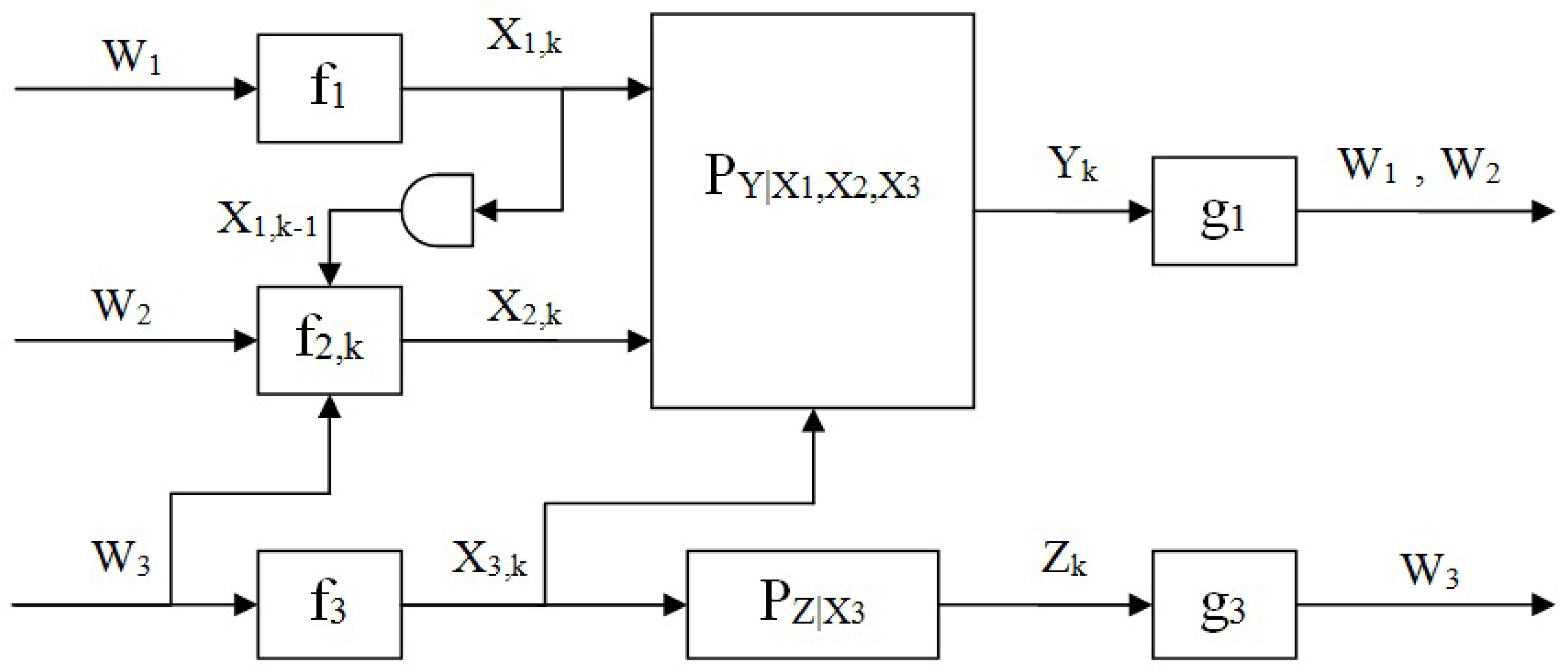
2. Channel Model and Preliminaries

Throughout this work, we will use uppercase letters (e.g., X) to denote random variables (RVs) and lowercase letters (e.g., x) to show their realization. Boldface letters are used for denoting n-vectors, e.g., x = x n = ( x 1 , . . . , x n ) . For a set of RVs S = { X 1 , . . . , X k } , A ϵ n ( S ) denotes the set of ϵ -strongly, jointly typical n-sequences of S as defined in ([40], Chapter 13). We may omit the index n from A ϵ n ( S ) when it is clear from the context.
A more formal definition of the problem is as follows: A discrete memoryless multiple-access Z-interference channel (MA-CZIC) is defined by the input alphabets ( X 1 , X 2 , X 3 ) and output alphabets ( Y , Z ) and by the transition probabilities P Y | X 1 , X 2 , X 3 and P Z | X 3 , that is, the channel outputs are generated in the following manner:
Pr y n , z n | x 1 n , x 2 n , x 3 n = t = 1 n p ( y t | x 1 , t , x 2 , t , x 3 , t ) p ( z t | x 3 , t ) .
Encoder i, i { 1 , 2 , 3 } , sends a message W i which is drawn uniformly over the set M i { 1 , , 2 n R i } to its destined receiver. It is further assumed that Encoder 2 “cribs” causally and observes the sequence of channel inputs emitted by Encoder 1 during all past transmissions before generating its next channel input. The model is depicted in Figure 1.
An ( 2 n R 1 , 2 n R 2 , 2 n R 3 , n ) code for the MA-CZIC with strictly causal Encoder 2 consists of:
  • Encoder 1 defined by a deterministic mapping
    f 1 : M 1 X 1 n
    which maps the message W 1 to a channel input codeword.
  • Encoder 2 which observes X 1 i 1 and W 3 prior to transmitting X 2 , i , is defined by the mappings
    f 2 , k ( s c ) : M 2 × M 3 × X 1 k 1 X 2 k = 1 , , n .
  • Encoder 3 is defined by a deterministic mapping
    f 3 : M 3 X 3 n .
  • The primary (main) decoder is defined by a mapping
    g 1 : Y n M 1 × M 2 .
  • The secondary decoder is defined by a mapping
    g 3 : Z n M 3 .
An ( 2 n R 1 , 2 n R 2 , 2 n R 3 , n ) code for the MA-CZIC with causal Encoder 2 differs only in the fact that Encoder 2 observes X 1 i (including the current symbol, X 1 , i ) before transmitting X 2 , i , and is defined by a the mappings
f 2 , k ( c ) : M 2 × M 3 × X 1 k X 2 k = 1 , 2 , , n .
For a given code, the block average error probability is
P e ( n ) = 1 2 n ( R 1 + R 2 + R 3 ) w 1 = 1 2 n R 1 w 2 = 1 2 n R 2 w 3 = 1 2 n R 3 Pr { g 1 ( Y n ) ( w 1 , w 2 ) g 3 ( Z n ) w 3 | W i = w i , i = 1 , 2 , 3 } .
A rate-triple ( R 1 , R 2 , R 3 ) is said to be achievable for the MA-CZIC if there exists a sequence of ( 2 n R 1 , 2 n R 2 , 2 n R 3 , n ) codes with lim n P e ( n ) = 0 . The capacity region of the MA-CZIC with a cribbing encoder is the closure of the set of achievable rate-triples.

3. Main Results

In this section, we provide inner and outer bounds to the capacity region of the discrete memoryless MA-CZIC.

3.1. Inner Bound

We next present achievable regions for the strictly causal and the causal MA-CZICs.
Definition 1.
Let R s c be the region defined by the closure of the convex hull of the set of all rate-triples ( R 1 , R 2 , R 3 ) satisfying
R 1 H ( X 1 | V )
R 2 I ( U ; Y | V L X 1 ) I ( U ; X 3 | V L )
R 1 + R 2 I ( V U X 1 ; Y | L ) I ( U ; X 3 | V L )
R 3 I ( X 3 ; Z | L ) + min { I ( L ; Y ) , I ( L ; Z ) }
for some probability distribution of the form
P V L U X 1 X 2 X 3 = P V P L P X 3 | L P X 1 | V P U X 2 | V L X 3 .
Theorem 1.
The region R s c is achievable for the MA-CZIC with a strictly causal cribbing encoder.
The proof appears in Appendix A.
Definition 2.
Let R c be the region defined by the closure of the convex hull of the set of all rate-triples ( R 1 , R 2 , R 3 ) satisfying (9a)–(9d), for some probability distribution of the form
P V L U X 1 X 2 X 3 = P V P L P X 3 | L P X 1 | V P U | V L X 3 P X 2 | U V L X 3 X 1 .
Theorem 2.
The region R c is achievable for the MA-CZIC with a causal cribbing encoder.
The outline of the proof appears in Appendix B.
A few comments regarding the achievability region (9a)–(9d) are in order. In the coding scheme, Encoder 1 and Encoder 2 use Block–Markov superposition encoding, while the primary decoder uses backward decoding [27]. In this scheme, the RV V represents the “resolution information” [26]; i.e., the current block information used for encoding the proceeding block. Encoder 3 uses rate-splitting, where the RV L represents the part of W 3 that can be decoded by both the primary and secondary decoders as can be observed by the term min { I ( L ; Y ) , I ( L ; Z ) } which appears in (9d). The complementary part of W 3 , while fully decoded by the secondary decoder, serves as a channel state for the primary channel in the form of X 3 . To reduce interference the cognitive encoder (Encoder 2) additionally uses Gel’fand–Pinsker binning [41] of U against X 3 , assuming an already successful decoding of V and L at the primary decoder, as can be seen in (9b).
It is important to note that the achievable region R s c is consistent with previously studied special cases: By setting R 1 = 0 and X 1 = 0 we can also set V = . The equations then reduce to
R 2 I ( U ; Y | L ) I ( U ; X 3 | L )
R 3 I ( X 3 ; Z | L ) + min { I ( L ; Y ) , I ( L ; Z ) } ,
and this results in the region achievable for the cognitive Z-Interference channel, studied in [36], with user 2 and user 3 as the cognitive and non-cognitive users, respectively.
Removing Encoder 2 by setting R 2 = 0 and X 2 = 0 we can also set U = and we get the classical Z-Interference channel with the 2 users, Encoder 1 and Encoder 3. In this case Y is dependent of V only through X 1 , since V X 1 Y , and I ( V U X 1 ; Y | L ) = I ( X 1 ; Y | L ) . We get
R 1 I ( X 1 ; Y | L )
R 3 I ( X 3 ; Z | L ) + min { I ( L ; Y ) , I ( L ; Z ) } .
An interesting setup arises by setting W 2 = 0 without removing Encoder 2. This models a relay channel, where Encoder 2 is a relay which has no message of its own and learns the information of the transmitter by cribbing (modeling excellent SNR conditions on this path). This model relates to [42], if the structure of the primary user ( X 3 ) is not accounted for, thus assuming i.i.d. state symbols known a-causally at the relay, as in [42].
Removing Encoder 3 by setting R 3 = 0 and X 3 = 0 we can also set L = , and the expression reduces to
R 1 H ( X 1 | V )
R 2 I ( U ; Y | V X 1 )
R 1 + R 2 I ( V U X 1 ; Y ) .
By setting U = X 2 we get the achievable region of the MAC with Encoder 2 as the cribbing encoder [26].
By setting L = 0 , removing inequality (9d) and replacing X 3 by S, whose given probability distribution is not to be optimized, the region reduces to the one in [27].
It is worth noting that in the case of a Gaussian channel, Encoder 2 can become fully cognitive of the message W 1 from a single sample of X 1 . This special case can be made non-trivial by adding a noisy channel or some deterministic function (quantizer for instance) between X 1 and Encoder 2.
Finally, we examine the case where Encoder 1’s output may be viewed as two parts X 1 = ( X 1 a , X 1 b ) where only the first part of the input affects the channel; i.e., P Y | X 1 X 2 X 3 = P Y | X 1 a X 2 X 3 . In this case, if the second part X 1 b is rich enough (e.g. continuous alphabet) Encoder 1 is able to transfer to Encoder 2 infinite amount of data, specifically the entire message W 1 . This is equivalent to the case of full cooperation from Encoder 1 to Encoder 2; i.e., the case where Encoder 2 has full knowledge of Encoder 1’s data W 1 . Hence, the cooperative state-dependent MAC where the state is known non-causally at the cognitive encoder [29] may also be considered as a special case of the MA-CZIC, when X 3 is replaced with an i.i.d. state S.

3.2. Outer Bound

In this section, we present an outer bound on the achievable region of the strictly causal and causal MA-CZIC.
Theorem 3.
Achievable rate-triples ( R 1 , R 2 , R 3 ) for the MA-CZIC with a strictly causal cribbing encoder belong to the closure of the convex hull of all rate triples that satisfy
R 1 H ( X 1 | V )
R 2 I ( U ; Y | V L X 1 ) I ( U ; Z | V L )
R 1 + R 2 I ( V U X 1 ; Y | L ) I ( V U ; Z | L )
R 3 I ( X 3 ; Z | L ) + min { I ( L ; Y ) , I ( L ; Z ) }
for some probability distribution of the form
P V L U X 1 X 2 X 3 = P X 3 P V P L | X 3 V P X 1 | V P U X 2 | V L X 3 .
The proof is provided in Appendix C, it is based on Fano’s Inequality [40] and from the Csiszár and Körner’s identity ([43], Lemma 7).
Theorem 4.
Achievable rate-triples ( R 1 , R 2 , R 3 ) for the MA-CZIC with a causal cribbing encoder belong to the closure of the convex hull of all rate regions given by (19a)–(19d) for some probability distribution of the form
P V L U X 1 X 2 X 3 = P X 3 P V P L | X 3 V P X 1 | V P U X 2 | V L X 3 X 1 .
The outline of the proof is provided in Appendix D.
As for the alphabet cardinalities: using standard applications of Carathéodory’s Theorem we obtain that it is sufficient to consider the alphabet cardinalities which are bounded as follows:
| L | | X 1 | | X 2 | | X 3 | + 4
| V | | X 1 | | X 2 | | X 3 | | L | + 3
| U | | X 1 | | X 2 | | X 3 | | L | | V | + 2 .
The details are omitted for the sake of brevity.

3.3. Special Cases

For the special case of a more-capable MA-CZIC channel we can actually establish the capacity region of the channel, both in the causal and the strictly causal cases.
Definition 3.
We say that the strictly-causal MA-CZIC is more-capable if I ( X 3 ; Y ) I ( X 3 ; Z ) for all probability distributions of the form P V P X 1 | V P X 3 P X 2 | V X 3 P Y | X 1 X 2 X 3 P Z | X 3 .
Theorem 5.
The capacity region of the more-capable strictly-causal MA-CZIC channel is the closure of the convex hull of the set of all rate-triples ( R 1 , R 2 , R 3 ) satisfying
R 1 H ( X 1 | V )
R 2 I ( X 2 ; Y | V X 1 X 3 )
R 1 + R 2 I ( X 1 X 2 ; Y | X 3 )
R 3 I ( X 3 ; Z )
for some probability distribution of the form
P V X 1 X 2 X 3 = P V P X 1 | V P X 3 P X 2 | V X 3 .
The proof of Theorem 5 is provided in Appendix E.
Theorem 6.
The capacity region of the more-capable causal MA-CZIC channel is the closure of the convex hull of the set of all rate-triples ( R 1 , R 2 , R 3 ) satisfying (25a)–(25d), for some probability distribution of the form
P V X 1 X 2 X 3 = P V P X 1 | V P X 3 P X 2 | V X 1 X 3 .
The proof of Theorem 6; i.e., the causal case, follows in the same manner as that of Theorem 5 and thus omitted.
Unfortunately, the requirement that the MA-CZIC is more-capable implies that the receiver Y has a better reception of the signal X 3 than its designated receiver Z, which is somewhat optimistic.
We next consider the cases where either one of the transmitters wishes to achieve its maximal possible rate; i.e., the vertex point of the capacity region.
Maximal rate at Transmitter 1:
Transmitter 2 may help Transmitter 1’s transmission and by doing so increase its rate. Therefore, we that assume Transmitter 2 dedicates its transmission to help transmitting W 1 . Transmitter 3 should minimize its interference at the Y Receiver. Setting L = X 3 , the entire interference caused by transmitter 3 at receiver 1 may be reduced via successive cancellation decoding. With no interference caused by transmitter 3, transmitter 2 may drop the Gelfand–Pinsker scheme, setting U = X 2 to maximize the rates. Thus, from (9a)–(9d) we get
R 1 min { H ( X 1 | V ) , I ( V X 1 X 2 ; Y | X 3 ) }
R 2 min { I ( X 2 ; Y | V X 1 X 3 ) ,      I ( V X 1 X 2 ; Y | X 3 ) R 1 }
R 3 min { I ( X 3 ; Y ) , I ( X 3 ; Z ) } .
From the Markov chain V X 1 X 2 X 3 Y we get I ( V X 1 X 2 ; Y | X 3 ) = I ( X 1 X 2 ; Y | X 3 ) . Therefore, we can rewrite (28a)–(28c) as
R 1 min { H ( X 1 | V ) , I ( X 1 X 2 ; Y | X 3 ) }
R 2 min { I ( X 2 ; Y | V X 1 X 3 ) ,      I ( X 1 X 2 ; Y | X 3 ) R 1 }
R 3 min { I ( X 3 ; Y ) , I ( X 3 ; Z ) } .
where in the strictly-causal MA-CZIC case, the union is over all probability distributions of the form
P V X 1 X 2 X 3 = P V P X 3 P X 1 | V P X 2 | V .
Maximal rate at Transmitter 2:
Both Transmitter 1 and 3 are not cognitive and have no knowledge of the message W 2 , thus they cannot help convey W 2 to Y and should only reduce their interference to a minimal level. Setting L = X 3 and U = X 2 follows as in maximizing R 1 in (28a)–(29c).
Therefore, we get (28a)–(28c) where the maximization is on R 2 instead of R 1 , i.e.
R 1 min { H ( X 1 | V ) , I ( X 1 X 2 ; Y | X 3 ) R 2 }
R 2 I ( X 2 ; Y | V X 1 X 3 )
R 3 min { I ( X 3 ; Y ) , I ( X 3 ; Z ) } .
Maximal rate at Transmitter 3:
Looking at (9d) and (19d) we see that the lower and upper bounds on R 3 coincide. Since transmitter 3 is not affected by the transmission of both transmitters 1 and 2, we can treat the transmitter 3—receiver 3 pair as a single user channel and thus achieve the Shannon capacity; i.e.,
R 3 I ( X 3 ; Z ) .
In the general case, the maximum rate at transmitter 3 is achieved by setting L = 0 . In this case, the higher rate at transmitter 3 comes at the expense of the other transmitters, since L was used for conveying part of the interference X 3 to Y. Thus, (9a)–(9d) become
R 1 H ( X 1 | V )
R 2 I ( U ; Y | V X 1 ) I ( U ; X 3 | V )
R 1 + R 2 I ( V U X 1 ; Y ) I ( U ; X 3 | V )
R 3 I ( X 3 ; Z ) .
Examining (9d), we see that maximum rate at transmitter 3 may also be achieved without affecting R 1 and R 2 . This is true when the receiver Y is less-noisy than receiver Z in the sense that I ( L ; Y ) I ( L ; Z ) for all probability distributions of the form (20). In this case (9d) becomes
R 3 I ( X 3 ; Z | L ) + min { I ( L ; Y ) , I ( L ; Z ) } = I ( X 3 ; Z | L ) + I ( L ; Z ) = I ( X 3 ; Z )
Actually, it suffices to require that the channel will be more-capable; i.e., I ( X 3 ; Y ) I ( X 3 ; Z ) for all probability distributions of the form (20), for achieving maximum rate at R 3 .

4. Cooperative Encoding

Let us now consider the case of full unidirectional cooperation from Encoder 1 to Encoder 2. This becomes a setup in which Encoders 1 and 2 share a common message, and Encoder 2 transmits a separate additional private message. Thus we have an interference cognitive channel (cognition in terms of W 3 ) with a common message, as depicted in Figure 2. Hence, Encoder 2 is given by the mapping
f 2 : M 1 × M 2 × M 3 X 2 n k = 1 , , n .
For this channel setup, a simpler outer bound on the capacity region can be derived providing some insights on the original problem. A special case of this channel, in which the secondary channel is removed and X 3 is replaced with an i.i.d. state S for the main channel; i.e., P Y | X 1 X 2 S , was studied in [29] and the single-letter characterization of the capacity region was established for that channel.
The following theorem provides a single-letter expression for an achievable region of the MA-CZIC with full unidirectional cooperation (common message).
Theorem 7.
The closure of the convex hull of the set of all rate-triples ( R 1 , R 2 , R 3 ) satisfying
R 1 + R 2 I ( X 1 U ; Y | L ) I ( U ; X 3 | L X 1 )
R 2 I ( U ; Y | L X 1 ) I ( U ; X 3 | L X 1 )
R 3 I ( X 3 ; Z | L ) + min { I ( L ; Y ) , I ( L ; Z ) }
for some probability distribution of the form
P L U X 1 X 2 X 3 = P X 1 P L P X 3 | L P U X 2 | X 1 L X 3
is achievable for the MA-CZIC with with full unidirectional cooperation.
The outline of the proof for Theorem 7 appears in Appendix F.
The following theorem provides a single-letter expression for an outer bound on the capacity region of the MA-CZIC with full unidirectional cooperation.
Theorem 8.
Achievable rate-triples ( R 1 , R 2 , R 3 ) for the MA-CZIC with full unidirectional cooperation belong to the closure of the convex hull of rate-regions given by
R 1 + R 2 I ( V U X 1 ; Y | L ) I ( V U ; Z | L )
R 2 I ( U ; Y | L V X 1 ) I ( U ; Z | L V )
R 3 I ( X 3 ; Z | L ) + min { I ( L ; Y ) , I ( L ; Z ) }
for some probability distribution of the form
P L V U X 1 X 2 X 3 = P V P X 3 P L | V X 3 1 { X 1 = f ( V ) } P U X 2 | V L X 3
The outline of the proof of Theorem 8 is provided in Appendix G.
Notice that inequalities (38a)–(38c) are identical to (19b)–(19d), where the probability distribution form (39) is a special case of (20). Thus, the outer bound established for R 2 , R 3 and the sum-rate R 1 + R 2 in the strictly-causal MA-CZIC, also holds for the case of full unidirectional cooperation. However, we would expect the outer bounds on R 2 and the sum-rate R 1 + R 2 to be smaller for the channel with the cribbing encoder, thus implying that the outer bound for the MA-CZIC is generally not tight.

5. Partial Cribbing

Next we consider the case of partial cribbing, where Encoder 2 views X 1 through a deterministic function
h : X 1 Y 2
instead of obtaining X 1 directly. This cribbing scheme is motivated by continuous input alphabet MA-CZIC, since perfect cribbing results in the degenerated case of full cooperation between the encoders and requires an infinite capacity link.
We define the strictly-causal MA-CZIC with partial cribbing as in (2)–(6) with the exception that Encoder 2 is defined by the mapping
f 2 , k ( s c ) : M 2 × M 3 × Y 2 k 1 X 2 k = 1 , , n
where y 2 , k = h ( x 1 , k ) for k = 1 , , n . The causal MA-CZIC with partial cribbing differs by setting
f 2 , k ( s c ) : M 2 × M 3 × Y 2 k X 2 k = 1 , , n .
It is worth noticing that the state-dependent MAC with state information known non-causally at one encoder [44] is a special case of the MA-CZIC with partial cribbing. This case is derived by setting h ( X 1 ) 0 and replacing X 3 with an i.i.d. state S. The capacity region of this simpler case remains an open problem. Therefore, it is hard to expect that capacity region would be established for the MA-CZIC with partial cribbing. Next, we establish inner and outer bounds for the MA-CZIC with partial cribbing.
Theorem 9.
The closure of the convex hull of the set of rate-triples ( R 1 , R 2 , R 3 ) satisfying
R 1 H ( Y 2 | V ) + I ( X 1 ; Y | V Y 2 U L )
R 2 I ( U ; Y | V L X 1 ) I ( U ; X 3 | V L )
R 1 + R 2 I ( V U X 1 ; Y | L ) I ( U ; X 3 | V L )
R 1 + R 2 I ( U X 1 ; Y | V L Y 2 ) + H ( Y 2 | V ) I ( U ; X 3 | V L )
R 3 I ( X 3 ; Z | L ) + min { I ( L ; Y ) , I ( L ; Z ) }
for some probability distribution of the form
P V L U X 1 Y 2 X 2 X 3 = P V P L P X 3 | L P X 1 Y 2 | V P U X 2 | V L X 3 .
is achievable for the strictly-causal MA-CZIC with partial cribbing.
The outline proof of Theorem 9 appears in Appendix H.
Theorem 10.
The closure of the convex hull of the set of rate-triples ( R 1 , R 2 , R 3 ) satisfying (43)–(47), for some probability distribution of the form
P V L U X 1 Y 2 X 2 X 3 = P V P L P X 3 | L P X 1 Y 2 | V P U | V L X 3 P X 2 | V Y 2 U L X 3 .
is achievable for the causal MA-CZIC with partial cribbing.
The proof of Theorem 10 is similar to that of Theorem 9 and thus is omitted.
Comparing this result to the achievability region found for the MA-CZIC we can see that inequalities (44), (45) and (47) are identical to (9b)–(9d), while inequality (43) differs and inequality (46) was added. In correspondence, the coding scheme for the MA-CZIC with partial cribbing differs from Theorem 1 mainly in Encoder 1. Encoder 1 now needs to transmit data in a lossy manner to both Y receiver and Encoder 2. To do so, Encoder 1 employs the rate-splitting technique. It splits its message W 1 into two parts ( W 1 a , W 1 b ) with rates R 1 a , R 1 b accordingly, such that R 1 = R 1 a + R 1 b . The rate R 1 a represents the rate of transmission to Encoder 2. Combining the rate-splitting with the superposition block Markov encoding (SBME) at Encoder 1 results in another codebook { y 2 n } , in addition to the two codebooks { v n } and { x 1 n } . The codebooks are created in an i.i.d. manner as follows: First, 2 n R 1 a codewords { v n } are created using P V . Then, for each codeword v n , 2 n R 1 a codewords { y 2 n } are drawn i.i.d. P Y 2 | V given v n . Finally, for each pair ( v n , y n ) , 2 R 1 b codewords { x n } are drawn i.i.d. P X 1 | Y 2 V given ( v n , y 2 n ) . Next, as in the scheme which corresponds to Theorem 1 SBME coding scheme, the index of the codeword y 2 n in time i becomes the index of v n in time i + 1 . For successful decoding at Encoder 2, we must require R 1 a H ( Y 2 | V ) . The rate R 1 a is therefore that of the information jointly transmitted to Y by both encoders. The remaining quantity in (43), that is, I ( X 1 ; Y | V Y 2 U L ) represents the rate R 1 b super-imposed by X 1 and decoded by Y via successive decoding. One may notice that in inequalities (44)–(45), the pair ( X 1 , Y 2 ) can replace X 1 , however since Y 2 is a deterministic function of X 1 it can be dropped.
This result is based on [28], where a capacity region was established for the case of the two-user MAC with cribbing through a deterministic function at both encoders.
Theorem 11.
Achievable rate-triples ( R 1 , R 2 , R 3 ) for the strictly-causal MA-CZIC with partial cribbing belong to a closure of the convex hull of the set of rate-regions given by
R 1 H ( Y 2 | V ) + I ( X 1 ; Y | V Y 2 U L )
R 2 I ( U ; Y | T L X 1 ) I ( U ; Z | T L )
R 1 + R 2 I ( T U X 1 ; Y | L ) I ( T U ; Z | L )
R 1 + R 2 I ( T U X 1 ; Y | V L Y 2 ) + H ( Y 2 | V ) I ( T U ; Z | V L )
R 3 I ( X 3 ; Z | L ) + min { I ( L ; Y ) , I ( L ; Z ) }
for some probability distribution of the form
P V L U T X 1 Y 2 X 2 X 3 = P T 1 { V = h ( T ) } P X 3 P L | T X 3 P X 1 | T 1 { Y 2 = h ( X 1 ) } P U X 2 | V L X 3 .
The proof of Theorem 11 as well as the following Theorem Theorem 12 appear in Appendix I.
Theorem 12.
Achievable rate-triples ( R 1 , R 2 , R 3 ) for the causal MA-CZIC with partial cribbing belong to the closure of the convex hull of the set of rate-regions given by (50)–(54), for some probability distribution of the form
P V L U T X 1 Y 2 X 2 X 3 = P T 1 { V = h ( T ) } P X 3 P L | T X 3 P X 1 | T 1 { Y 2 = h ( X 1 ) } P U X 2 | V L X 3 X 1 .
It is easy to see that setting h ( · ) to be the identity function, T = V and Y 2 = X 1 , the region of Theorem 11 degenerates to the outer bound of the MA-CZIC with noiseless cribbing (Theorem 3).
A related problem is the Cognitive State-Dependent MAC with Partial Cribbing. This setup is obtained by removing user 3 and replacing X 3 with an i.i.d. state S known non-causally at Encoder 2. From the inner bound (Theorem 9) and outer bound (Theorem 11) for the MA-CZIC with partial cribbing derived in previous sections it is immediate to derive inner and outer bounds for the channel by setting L = 0 and X 3 = Z = S . Doing so yields the following inner and outer bounds.
Theorem 13.
The closure of the convex hull of the set of rate-pairs ( R 1 , R 2 ) satisfying
R 1 H ( Y 2 | V ) + I ( X 1 ; Y | V Y 2 U )
R 2 I ( U ; Y | V X 1 ) I ( U ; S | V )
R 1 + R 2 I ( V U X 1 ; Y ) I ( U ; S | V )
R 1 + R 2 I ( U X 1 ; Y | V Y 2 ) + H ( Y 2 | V ) I ( U ; S | V )
for some probability distribution of the form
P V L U X 1 Y 2 X 2 S = P V P S P X 1 Y 2 | V P U X 2 | V S
is achievable for the state-dependent cognitive MAC with partial (strictly-causal) cribbing.
Theorem 14.
Achievable rate-pairs ( R 1 , R 2 ) for the state-dependent cognitive MAC with partial (strictly-causal) cribbing belong to the closure of the convex hull of rate-regions given by
R 1 H ( Y 2 | V ) + I ( X 1 ; Y | V Y 2 U )
R 2 I ( U ; Y | T X 1 ) I ( U ; S | T )
R 1 + R 2 I ( T U X 1 ; Y ) I ( T U ; S )
R 1 + R 2 I ( T U X 1 ; Y | V Y 2 ) + H ( Y 2 | V ) I ( T U ; S | V )
for some probability distribution of the form
P V U T X 1 Y 2 X 2 S = P T 1 { V = h ( T ) } P S P X 1 | T 1 { Y 2 = h ( X 1 ) } P U X 2 | V S .

6. Discussion and Future Work

The use of cognitive radio holds tremendous promise in better exploiting the available spectrum. Sensing its environment, a cognitive radio can use it as network side information resulting in better performances for all users. The cognitive transmitter may use this information to reduce interference at its end, reduce interference for the other users or help relaying information. However, obtaining this side-information is not always practical in actual scenarios. The assumption of a-priori knowledge of the other user’s information may only be applied to certain situations where the transmitters share information through a separate channel. The assumption of causally sensing the environment is more realistic in many cases of distinct transmitters. Nevertheless, the cognitive transmitter will most likely acquire a noisy version of the information limiting its ability to cooperate. In addition, sensing the environment involves complicated implementations of the transmitter as well as power consumption for which the cognition improvement is weighed against. Nevertheless, the improved transmission rates achieved via cognitive schemes motivate their integration into various wireless systems such as Wi-Fi and Cellular networks. We note that cribbing requires parallel receiver/transmit technology (duplex operation), which is useful and usually available, as in the 5G systems. Although receiving much attention recently ([15,16]), many of the fundamental problems of cognitive multi-terminal networks remain unsolved.
In this paper we investigated some cognitive aspects of multi-terminal communication networks. We introduced the MA-CZIC as generalization of a compound cognitive multi-terminal network. The MA-CZIC incorporates various multi-terminal communication channels—MAC, Z-IFC—as well as several cognition aspects—cooperation and cribbing. For the MA-CZIC we have drawn inner and outer bounds on its capacity region. In an effort to better characterize the capacity region, we studied the extreme points of the achievability region, and were able to find the capacity region in the case the channel is more-capable. Furthermore, we investigated some variations of the channel regarding the nature of cooperation between the cognitive encoder—Encoder 2—and the non-cognitive encoder sharing its receiver—Encoder 1. The case in which Encoder 2 has better cognition abilities and obtains full knowledge of Encoder 1’s message was investigated. Furthermore, the case where Encoder 2 has worse cognition abilities and cribs from Encoder 1 via a deterministic function, such as quantizer, was studied.
As for possible future work, several directions can be considered. First, it would be interesting to identify some concrete non-trivial channel specification for which the MA-CZIC inner and outer bounds coincide, at least in partial regions. Finding such a channel may help us get insight about the capacity region as well as the margins given by the inner and outer bounds. Moreover, the characterization of the capacity region may be further improved by examining different interference regimes. Determining the exact capacity region for the MA-CZIC will subsequently result in the capacity region for the cognitive Z-IFC [36] as a special case. We believe that the opposite derivation also applies; i.e., the capacity region of the MA-CZIC will follow from the capacity region of the cognitive Z-IFC. Our model assumed that the cognitive transmitter—transmitter 2—has full non-causal knowledge of the interference signal X 3 . While modeling the interference signal as a transmitter is very realistic in many scenarios, the assumption of non-causal knowledge of the signal, may not hold in practice in case the cognitive transmitter has sensing capabilities but not shared information. Therefore, the model where transmitter 2 cribs from transmitter 3 is very much in place, and it would be very interesting to see if it is possible to determine the capacity region for the channel. Possible iprovement of the achievable bounds may incorporate the fact that X 3 is associated with a coding scheme, and hence the interference can be mitigated by partial/full decoding, with possible aid of the cognizant transmitter 2.

Acknowledgments

This work was supported by the Heron consortium via the Israel ministry of economy and science.

Author Contributions

All three authors cooperated in the theoretical research leading to the reported results and in composing this submitted paper.

Conflicts of Interest

The founding sponsors had no role in the design of the study; in the collection, analyses, or interpretation of data; in the writing of the manuscript, and in the decision to publish the results.

Abbreviations

The following abbreviations are used in this manuscript:
MACMultiple-Access Channel
IFCInterference Channel
OFDMAOrthogonal Frequency-Division Multiple Access
HKHan-Kobayashi
QoSQuality of Service
DFDecode and Forward
AFAmplify and Forward
CIFCCognitive Interference Channel
MA-CZICMultiple-Access Cognitive Z-Interference Channel
P2Ppoint-to-point
RVRandom Variable
AEPAsymptotic Equipartition Property

Appendix A

Proof of Theorem 1.
Below is a description of the random coding scheme we use to prove achievability of rate-triples in R s c , the analysis of the average probability of error is omitted.
We propose the following coding scheme, which includes Block–Markov superposition coding, backward decoding, rate splitting and Gelfand–Pinsker coding [41]. The coding scheme combines the coding techniques of [36] with that of [27], which, in turn, is based on the coding technique of [26,29].
For a fixed distribution P V P L P X 3 | L P X 1 | V P U X 2 | V L X 3 the coding schemes are as follows:

Appendix A.1. Encoder 3 and Decoder 3 Coding Scheme

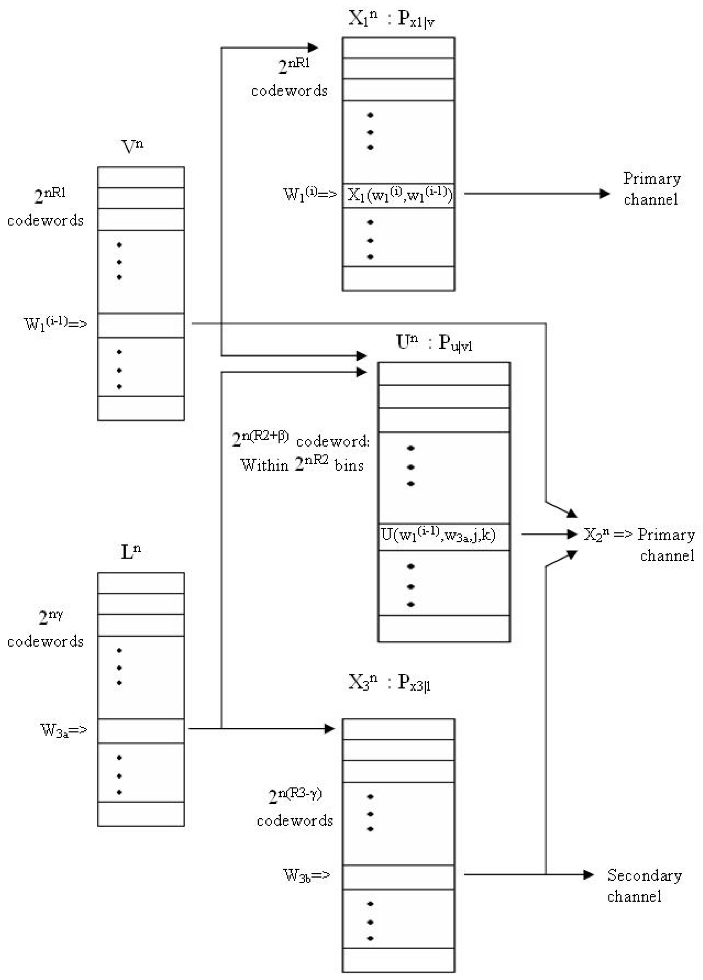
Appendix A.1.1. Encoder 3 Codebook generation

Generate independently 2 n γ codewords l = ( l 1 , , l n ) , each with probability Pr ( l ) = i = 1 n p L ( l i ) . These codewords constitute the inner codebook of Transmitter 3. Denote them as l ( k ) where k { 1 , , 2 n γ } . For each codeword l ( k ) , generate 2 n ( R 3 γ ) codewords x 3 = ( x 3 , 1 , , x 3 , n ) , each with probability Pr ( x 3 | l ( k ) ) = i = 1 n P X 3 | L ( x 3 , i | l i ( k ) ) . Denote them as x 3 ( j , k ) , j = 1 , , 2 n ( R 3 γ ) . The codewords { x 3 ( j , k ) } j = 1 2 n ( R 3 γ ) constitute the outer codebook of Transmitter 3 associated with the codeword l ( k ) .

Appendix A.1.2. Encoding Scheme of Encoder 3

Encoder 3 splits its message W 3 into two independent parts W 3 = ( W 3 a , W 3 b ) , with rates γ and R 3 γ respectively. For W 3 a = w 3 a and W 3 b = w 3 b it transmits x 3 ( w 3 a , w 3 b ) .

Appendix A.1.3. Receiver 3 Decoding

Receiver 3 looks for w ^ 3 = ( w ^ 3 a , w ^ 3 b ) such that
l ( w ^ 3 a ) , x 3 ( w ^ 3 a , w ^ 3 b ) , z A ϵ ( L , X 3 , Z ) .
If no such w ^ 3 exists an error is declared, and if there exists more than one w ^ 3 that satisfies the condition, the decoder chooses w ^ 3 at random among them.

Appendix A.2. Encoder 1, Encoder 2 and Main Decoder Coding Scheme

We consider B Blocks, each of n symbols. A sequence of B 1 message pairs ( W 1 ( b ) , W 2 ( b ) ) for b = 1 , . . . , B 1 , will be transmitted during B transmission blocks. As B , for a fixed n, the rate pair of the message ( W 1 , W 2 ) , ( R ˜ 1 , R ˜ 2 ) = ( R 1 ( B 1 ) / B , R 2 ( B 1 ) / B ) converges to ( R 1 , R 2 ) .

Appendix A.2.1. Encoder 1 Codebook generation

Generate 2 n R 1 codewords v = ( v 1 , , v n ) , each with probability Pr ( v ) = i = 1 n P V ( v i ) . These codewords constitute the inner codebook of Transmitter 1. Denote them as v ( w 0 ) , where w 0 { 1 , , 2 n R 1 } . For each codeword v ( w 0 ) generate 2 n R 1 codewords x 1 , each with probability Pr ( x 1 | v ( w 0 ) ) = i = 1 n P X 1 | V ( x 1 , i | v i ( w 0 ) ) . These codewords, { x 1 } , constitute the outer codebook of Transmitter 1 associated with v ( w 0 ) . Denote them as x 1 ( w 1 , w 0 ) where w 0 is as before, representing the index of the codeword v ( w 0 ) in the inner codebook and w 1 { 1 , , 2 n R 1 } the index of the codeword x 1 in the associated outer codebook.

Appendix A.2.2. Encoding Scheme of Encoder 1

Given W 1 ( b ) = w 1 ( b ) { 1 , , 2 n R 1 } for b = 1 , 2 , , B , we define w 0 ( b + 1 ) = w 1 ( b ) for b = 1 , 2 , , B 1 .
In block 1 Encoder 1 sends
x 1 ( 1 ) = x 1 ( w 1 ( 1 ) , 1 ) ,
in block b = 2 , 3 , , B 1 Encoder 1 sends
x 1 ( b ) = x 1 ( w 1 ( b ) , w 0 ( b ) )
and in block B Encoder 1 sends
x 1 ( B ) = x 1 ( 1 , w 0 ( B ) )

Appendix A.2.3. Encoder 2 Codebook Generation

This encoder’s codebook is based on both Encoder 1 and Encoder 3 inner codebooks. For each two codewords v ( w 0 ) and l ( k ) generate 2 n ( R 2 + β ) codewords u = ( u 1 , , u n ) , each with probability Pr ( u | v ( w 0 ) l ( k ) ) = i = 1 n p U | V L ( u i | v i ( w 0 ) l i ( k ) ) . These codewords constitute Encoder 2’s codebook associated with v ( w 0 ) and l ( k ) . Randomly partition each of the codebooks into 2 n R 2 bins, each consisting of 2 n β codewords. Now label the codewords by u ( w 0 , w 2 , w 3 a , t ) , where the codebook is chosen according to v ( w 0 ) and l ( w 3 a ) , w 2 { 1 , , 2 n R 2 } defines the bin according to Encoder 2’s message, and t { 1 , , 2 n β } is the index within the bin.

Appendix A.2.4. Encoding Scheme of Encoder 2

Given ( w 0 ( b ) , w 1 ( b ) , w 3 ( b ) ) as before and W 2 ( b ) = w 2 ( b ) { 1 , , 2 n R 2 } , search for the lowest t { 1 , , 2 n β } such that u ( b ) = u ( w 0 ( b ) , w 2 ( b ) , w 3 a ( b ) , t ) is jointly typical with the triplet v ( w 0 ( b ) ) , l ( w 3 a ( b ) ) , x 3 ( w 3 ( b ) ) , denoting that t as t ( w 0 ( b ) , w 2 ( b ) , w 3 ( b ) ) . If such a t is not found or if the triplet v ( w 0 ( b ) ) , l ( w 3 a ( b ) ) , x 3 ( w 3 ( b ) ) is not jointly typical, an error is declared and t ( w 0 ( b ) , w 2 ( b ) , w 3 ( b ) ) = 1 . Now, create the codeword x 2 ( b ) = x 2 ( w 0 ( b ) , w 2 ( b ) , w 3 ( b ) ) by drawing its components i.i.d. conditionally on the quadruple v ( w 0 ( b ) ) , l ( w 3 a ( b ) ) , u ( w 0 ( b ) , w 2 ( b ) , w 3 a ( b ) , t ) , x 3 ( w 3 ( b ) ) , where the conditional law is induced by (10).
In block 1 Encoder 2 sends
x 2 ( 1 , w 2 ( 1 ) , w 3 ( 1 ) ) .
As a result of cribbing from Encoder 1, before the beginning of block b = 2 , 3 , , B , Encoder 2 has an estimate w ^ ^ 0 ( b ) for w 0 ( b ) . Then, for b = 2 , 3 , , B 1 , Encoder 2 sends
x 2 ( w ^ ^ 0 ( b ) , w 2 ( b ) , w 3 ( b ) )
and in block B Encoder 2 sends
x 2 ( w ^ ^ 0 ( B ) , 1 , w 3 ( B ) ) .
Schematic description of the encoding appears in Figure A1.
Figure A1. A schematic description of the codebooks hierarchy and encoding procedure at the three encoders.
Entropy 19 00378 g003

Appendix A.2.5. Decoding at the Primary Receiver ( g 1 )

After receiving B blocks the decoder uses backward decoding starting from decoding block B moving on downward to block 1. In block B the receiver looks for w ^ 0 ( B ) = w ^ 1 ( B 1 ) such that
v ( w ^ 1 ( B 1 ) ) , x 1 ( 1 , w ^ 1 ( B 1 ) ) , u ( w ^ 1 ( B 1 ) , 1 , w 3 a ( B ) , t ) , l ( w 3 a ( B ) ) , y ( B ) A ϵ ( V , X 1 , U , L , Y )
for some w 3 a ( B ) , where t = t ( w ^ 1 ( B 1 ) , 1 , w 3 ( b ) ) .
At block b = 1 , 2 , , B 1 , assuming that a decoding was done backward down to (and including) block b + 1 , the receiver decoded w ^ 1 ( B 1 ) , ( w ^ 2 ( B 1 ) , w ^ 1 ( B 2 ) ) , , ( w ^ 2 ( b + 1 ) , w ^ 1 ( b ) ) . Then, to decode block b, the receiver looks for ( w ^ 2 ( b ) , w ^ 1 ( b 1 ) ) such that
v ( w ^ 1 ( b 1 ) ) , x 1 ( w ^ 1 ( b ) , w ^ 1 ( b 1 ) ) , u ( w ^ 1 ( b 1 ) , w ^ 2 ( b ) , w 3 a ( b ) , t ) , l ( w 3 a ( b ) ) , y ( b ) A ϵ ( V , X 1 , U , L , Y )
for some w 3 a ( b ) , where t = t ( w ^ 1 ( b 1 ) , w ^ 2 ( b ) , w 3 ( b ) ) .

Appendix A.2.6. Decoding at Encoder 2

To obtain cooperation, after block b = 1 , 2 , , B 1 , Encoder 2 chooses w ˜ 1 ( b ) such that
v ( w ˜ 0 ( b ) ) , x 1 ( w ˜ 1 ( b ) , w ˜ 0 ( b ) ) , x 1 ( b ) A ϵ ( V , X 1 , X 1 )
where w 0 ˜ ( b ) = w ˜ 1 ( b 1 ) was determined at the end of block b 1 and w ˜ 0 ( 1 ) = 1 .
At each of the decoders, if a decoding step either fails to recover a unique index (or index pair) which satisfies the decoding rule, or there is more than one index (or index pair), then an index (or index pair) is chosen at random among the indices which satisfies the decoding rule.
It can be shown that the error probability will be arbitrarily small if (9a)–(9d) hold.

Appendix A.3. Bounding the Probability of Error

We define the error events E 0 ( b ) E 7 ( b ) as follows:
  • E 0 ( b ) : Codebook error, the codewords v , x 1 , l , x 3 are not jointly typical. That is
    v ( w 0 ( b ) ) , x 1 ( w 1 ( b ) , w 0 ( b ) ) A ϵ ( V , X 1 ) l ( w 3 a ( b ) ) , x 3 ( w 3 a ( b ) , w 3 b ( b ) ) A ϵ ( L , X 3 )
  • E 1 ( b ) : Error decoding w 1 ( b ) at Encoder 2, that is, there exists w ˜ 1 ( b ) w 1 ( b ) such that
    v ( w 0 ( b ) ) , x 1 ( w ˜ 1 ( b ) , w 0 ( b ) ) , x 1 ( b ) A ϵ ( V , X 1 , X 1 )
  • E 2 ( b ) : Encoding error at Encoder 2, no suitable encoding index t. That is, there is no t { 1 , , 2 n β } such that
    v ( w 0 ( b ) ) , l ( w 3 a ( b ) ) , u ( w 0 ( b ) , w 2 ( b ) , w 3 a ( b ) , t ) , x 3 ( w 3 a ( b ) , w 3 b ( b ) ) A ϵ ( V , L , U , X 3 )
  • E 3 ( b ) : Channel error, one or more of the input signals is not jointly typical with the outputs y and z . That is
    v ( w 0 ( b ) ) , u ( w 0 ( b ) , w 2 ( b ) , w 3 a ( b ) , t ) , x 1 ( w 1 ( b ) , w 0 ( b ) ) , l ( w 3 a ( b ) ) , x 3 ( w 3 a ( b ) , w 3 b ( b ) ) , y ( b ) , z ( b ) A ϵ ( V , U , X 1 , L , X 3 , Y , Z )
  • E 4 ( b ) : Codebook error in decoding w 3 a ( b ) at either one of the decoders, a false message was detected. That is, there exists w ˜ 3 a ( b ) w 3 a ( b ) such that
    l ( w ˜ 3 a ( b ) ) , y ( b ) A ϵ ( L , Y ) l ( w ˜ 3 a ( b ) ) , z ( b ) A ϵ ( L , Z )
  • E 5 ( b ) : Codebook error in decoding w 0 ( b ) . There exists w ˜ 0 ( b ) w 0 ( b ) such that
    v ( w ˜ 0 ( b ) ) , u ( w ˜ 0 ( b ) , j , w 3 a ( b ) , t ) , x 1 ( w 1 ( b ) , w ˜ 0 ( b ) ) , l ( w 3 a ( b ) ) , y ( b ) A ϵ ( V , U , X 1 , L , Y )
    for some pair ( j , t ) j W 2 , t { 1 , , 2 n β } .
  • E 6 ( b ) : Codebook error in decoding w 2 ( b ) . There exists a different bin w ˜ 2 ( b ) w 2 ( b ) , such that
    v ( w 0 ( b ) ) , u ( w 0 ( b ) , w ˜ 2 ( b ) , w 3 a ( b ) , t ) , x 1 ( w 1 ( b ) , w 0 ( b ) ) , l ( w 3 a ( b ) ) , y ( b ) A ϵ ( V , U , X 1 , L , Y )
    for some t { 1 , , 2 n β } .
  • E 7 ( b ) : Codebook error in decoding w 3 b ( b ) . There exists w ˜ 3 b ( b ) w 3 b ( b ) such that
    l ( w 3 a ( b ) ) , x 3 ( w 3 a ( b ) , w ˜ 3 b ( b ) ) , z ( b ) A ϵ ( L , X 3 , Z )
Notice that when Encoder 2 observes x 1 error-free, as in this setup, the error event E 1 ( b ) (A1) can be replaced with the explicit case of having two identical codewords in { x 1 } codebook, i.e, there exists w ˜ 1 ( b ) w 1 ( b ) such that x 1 ( w ˜ 1 ( b ) , w 0 ( b ) ) = x 1 ( b ) .
We now define the events F i , i = 0 5 as follows:
  • F 0 b = 1 B E 0 ( b )
  • F 1 b = 1 B ( E 0 ( b ) E 1 ( b ) )
  • F 2 b = 1 B ( E 0 ( b ) E 1 ( b ) E 2 ( b ) )
  • F 3 b = 1 B ( E 0 ( b ) E 1 ( b ) E 2 ( b ) E 3 ( b ) )
  • F 4 b = 1 B ( E 0 ( b ) E 1 ( b ) E 2 ( b ) E 3 ( b ) E 4 ( b ) )
  • F 5 ( b ) i = 5 7 E i ( b ) , b = 1 , . . . , B
We upper bound the average probability of error P ¯ e averaged over all codebooks and all random partitions, as in [27], by
P ¯ e b = 1 B { Pr [ E 0 ( b ) ] + Pr [ E 1 ( b ) | F 0 c , E 1 ( 1 . . . b 1 ) C ] } + b = 1 B { Pr [ E 2 ( b ) | F 1 c ] + Pr [ E 3 ( b ) | F 2 c , E 3 ( 1 . . . b 1 ) C ] } + b = 1 B { Pr [ E 4 ( b ) | F 3 c ] + Pr [ F 5 ( b ) | F 4 c , F 5 ( b + 1 . . . B ) C ] }
where F ( 1 b 1 ) C denotes the complement of the event i = 1 b 1 F ( i ) .
Furthermore, we can upper bound each of the summands in the last component of (A3) by the union bound as
Pr [ F 5 ( b ) | F 4 c , F 5 ( b + 1 . . . B ) C ] = Pr i = 5 7 E i ( b ) | F 4 c , F 5 ( b + 1 . . . B ) C i = 5 7 Pr ( E i ( b ) | F 4 c , F 5 ( b + 1 . . . B ) C ) .
Now, we can separately examine and upper bound each of the summands in (A3):
  • By the Asymptotic Equipartition Property (AEP) [40], Pr [ E 0 ( b ) ] 0 as n .
  • In the second summand, Pr [ E 1 ( b ) | F 0 c , E 1 ( 1 . . . b 1 ) C ] , the conditioning on F 0 c , E 1 ( 1 . . . b 1 ) C insures that ( x 1 ( b ) , v ( b ) ) are jointly typical, and that Encoder 2 decoded correctly all the previous messages w 1 ( 1 ) , , w 1 ( b 1 ) and specifically w 0 ( b ) ( = w 1 ( b 1 ) ) . Since each codeword x 1 ( · , w 0 ( b ) ) is drawn i.i.d. given w 0 ( b ) , from the strong typicality Lemma we get
    P r [ E 1 , j ( b ) | F 0 c , E 1 ( 1 . . . b 1 ) C ] 2 n [ H ( X 1 | V ) ϵ ] , j w 1 ( b )
    where E 1 , j ( b ) is the event
    v ( w 0 ( b ) ) , x 1 ( j , w 0 ( b ) ) , x 1 ( b ) A ϵ ( V , X 1 , X 1 ) .
    Assuming, without loss of generality, that w 1 ( b ) = 1 , we get by using the union bound
    Pr [ E 1 ( b ) | F 0 c , E 1 ( 1 . . . b 1 ) C ] j = 2 2 n R 1 P r [ E 1 , j ( b ) | F 0 c , E 1 ( 1 . . . b 1 ) C ] ( 2 n R 1 1 ) × 2 n [ H ( X 1 | V ) ϵ ] .
    Hence for
    R 1 H ( X 1 | V ) ϵ
    we get Pr [ E 1 ( b ) | F 0 c , E 1 ( 1 . . . b 1 ) C ] 0 as n .
  • Since the codewords { u } are generated in an i.i.d. manner we have
    E 2 ( b ) = t = 1 2 n β E 2 , t ( b )
    where E 2 , t ( b ) is the event
    v ( w 0 ( b ) ) , l ( w 3 a ( b ) ) , u ( w 0 ( b ) , w 2 ( b ) , w 3 a ( b ) , t ) , x 3 ( w 3 ( b ) ) A ϵ ( V , L , U , X 3 )
    for a specific index t. Hence, we have
    Pr [ E 2 ( b ) | F 1 c ] = t = 1 2 n β Pr [ E 2 , t ( b ) | F 1 c ] .
    Conditioning on V and L in ([41], Lemma 3) we get
    Pr [ E 2 , t ( b ) | F 1 c ] 1 2 n [ I ( U ; X 3 | V L ) + ϵ 1 ]
    for all t { 1 , , 2 n β } , where ϵ 1 0 as ϵ 0 . Hence
    Pr [ E 2 ( b ) | F 1 c ] ( 1 2 n [ I ( U ; X 3 | V L ) + ϵ 1 ] ) 2 n β .
    The expression converges to 0 as n for
    β > I ( U ; X 3 | V L ) + ϵ 1 .
  • By the AEP Pr [ E 3 ( b ) | F 2 c , E 3 ( 1 . . . b 1 ) C ] 0 as n .
  • If
    γ min { I ( L ; Y ) , I ( L ; Z ) }
    then, from joint typicality decoding, Pr [ E 4 ( b ) | F 3 c ] 0 as n .
  • We state that
    Pr [ E 5 ( b ) | F 4 c , F 5 ( b + 1 . . . B ) C ] i = 1 2 n R 1 j = 1 2 n R 2 t = 1 2 n β Pr [ E 5 , i j t ( b ) | F 4 c , F 5 ( b + 1 . . . B ) C ]
    where E 5 , i j t ( b ) stands for the event
    v ( i ) , u ( i , j , w 3 a ( b ) , t ) , x 1 ( w 1 ( b ) , i ) , l ( w 3 a ( b ) ) , y ( b ) A ϵ ( V , U , X 1 , L , Y ) .
    By using the strong typicality Lemma we bound each of the summands above
    Pr [ E 5 , i j t ( b ) | F 4 c , F 5 ( b + 1 . . . B ) C ] 2 n [ H ( V U X 1 L Y ) + ϵ ] 2 n [ H ( V U X 1 L ) ϵ ] 2 n [ H ( Y | L ) ϵ ] = 2 n [ I ( U V X 1 ; Y | L ) 3 ϵ ] .
    Summing over all codewords we get
    Pr [ E 5 ( b ) | F 4 c , F 5 ( b + 1 . . . B ) C ] 2 n [ I ( U V X 1 ; Y | L ) + 3 ϵ ] 2 n ( R 1 + R 2 + β ) .
    Therefore, if
    R 1 + R 2 + β I ( V U X 1 ; Y | L ) + 3 ϵ
    then Pr [ E 5 ( b ) | F 4 c , F 5 ( b + 1 . . . B ) C ] 0 as n .
  • Similarly, using the same technique as the previous step, if
    R 2 + β I ( U ; Y | V L X 1 ) + 3 ϵ
    then Pr [ E 6 ( b ) | F 4 c , F 5 ( b + 1 . . . B ) C ] 0 as n .
  • Finally, if
    R 3 γ I ( X 3 ; Z | L )
    then Pr [ E 7 ( b ) | F 4 c , F 5 ( b + 1 . . . B ) C ] 0 as n .
From (A7)–(A16) we get (9a)–(9d), thus concluding the proof. ☐

Appendix B

Outline of the Proof of Theorem 2:
The achievability part follows similarly to that of Theorem 1, the only difference being in the way the codeword x 2 ( w ^ ^ 0 ( b ) , w 2 ( b ) , w 3 ( b ) ) is generated. Here, the second encoder generates the codeword x 2 ( w ^ ^ 0 ( b ) , w 2 ( b ) , w 3 ( b ) ) by drawing its components i.i.d. conditionally on the quintuple v ( w 0 ( b ) ) , l ( w 3 a ( b ) ) , u ( b ) , x 3 ( b ) , x 1 ( b ) , where the conditional law is induced by (11).

Appendix C

Proof of Theorem 3—Strictly Causal MA-CZIC Outer Bound.
Consider an ( 2 n R 1 , 2 n R 2 , 2 n R 3 , n ) code with average block error probability P e ( n ) = n ϵ n , and a probability distribution on W 1 × W 2 × W 3 × X 1 × X 2 × X 3 × Y × Z given by
p W 1 W 2 W 3 X 1 n X 2 n X 3 n Y n Z n = p W 1 p W 2 p W 3 1 { X 1 n = f 1 ( W 1 ) } 1 { X 3 n = f 3 ( W 3 ) } · i = 1 n p X 2 i | W 2 W 3 X 1 i 1 p Y i | X 1 i X 2 i X 3 i p Z i | X 3 i .
For i { 1 , 2 , , n } , let V i , L i and U i be the random variables defined by
V i X 1 i 1 , L i ( Y i 1 , Z i + 1 n ) , U i W 2 .
and let U be the random variable defined by further defining Q to be an auxiliary (time-sharing) random variable that is distributed uniformly on the set { 1 , 2 , , n } , and let
V ( V Q , Q ) , X 1 X 1 Q , L ( L Q , Q ) , X 3 X 3 Q , Y Y Q , Z Z Q , U U Q .
We start with an upper bound on R 1
n R 1 = H ( W 1 | W 2 ) = I ( W 1 ; Y n | W 2 ) + H ( W 1 | W 2 Y n ) I ( W 1 ; Y n | W 2 ) + n ϵ n = ( a ) I ( X 1 n ; Y n | W 2 ) + n ϵ n = i = 1 n I ( X 1 i ; Y n | W 2 X 1 i 1 ) + n ϵ n i = 1 n H ( X 1 i | X 1 i 1 ) + n ϵ n = i = 1 n H ( X 1 i | V i ) + n ϵ n = H ( X 1 Q | V Q Q ) + n ϵ n = H ( X 1 | V ) + n ϵ n ,
where ( a ) follows from the encoding relation in (2).
Next, consider R 3
n R 3 = H ( W 3 ) = I ( W 3 ; Z n ) + H ( W 3 | Z n ) I ( W 3 ; Z n ) + n ϵ n = H ( Z n ) H ( Z n | W 3 ) + n ϵ n ( b ) H ( Z n ) H ( Z n | W 3 X 3 n ) + n ϵ n = ( c ) H ( Z n ) H ( Z n | X 3 n ) + n ϵ n = ( d ) H ( Z n ) i = 1 n H ( Z i | X 3 i ) + n ϵ n ,
where ( b ) follows from the fact that conditioning decreases entropy, ( c ) follows from the Markov chain W 3 X 3 n Z n and ( d ) follows since the channel P Z | X 3 is memoryless.
Using the Csiszár-Körner’s identity ([43], Lemma 7) we obtain
H ( Y n ) H ( Z n ) = i = 1 n [ H ( Y i | Y i 1 Z i + 1 n ) H ( Z i | Y i 1 Z i + 1 n ) ] = i = 1 n [ H ( Y i | L i ) H ( Z i | L i ) ] ,
where the last equality follows from (A18). Substituting (A19) into (A22) we get
1 n ( H ( Y n ) H ( Z n ) ) = H ( Y | L ) H ( Z | L ) .
Notice that (A23) implies that there exists a number γ where
γ = 1 n H ( Y n ) H ( Y | L ) = 1 n H ( Z n ) H ( Z | L )
0 γ min { I ( L ; Y ) , I ( L ; Z ) }
where the right inequality of (A25) follows since H ( Y n ) n H ( Y ) and H ( Z n ) n H ( Z ) , and the left inequality follows since
H ( Y n ) = i = 1 n H ( Y i | Y i 1 ) i = 1 n H ( Y i | Y i 1 Z i + 1 n ) = n H ( Y | L ) .
Following from (A21) we have
R 3 1 n H ( Z n ) 1 n i = 1 n H ( Z i | X 3 i ) + ϵ n = ( e ) H ( Z | L ) + γ H ( Z | X 3 Q ) + ϵ n = ( f ) H ( Z | L ) + γ H ( Z | X 3 ) + ϵ n H ( Z | L ) H ( Z | X 3 ) + min { I ( L ; Y ) , I ( L ; Z ) } + ϵ n = ( g ) H ( Z | L ) H ( Z | X 3 L ) + min { I ( L ; Y ) , I ( L ; Z ) } + ϵ n = I ( X 3 ; Z | L ) + min { I ( L ; Y ) , I ( L ; Z ) } + ϵ n ,
where ( e ) follows from (A24) and the definitions of random variables in (A19); ( f ) follows since the channel P Z | X 3 is memoryless, and ( g ) follows from the Markov chain L X 3 Z .
Next, consider R 2
R 2 = 1 n H ( W 2 | W 1 ) 1 n I ( W 2 ; Y n | W 1 ) + ϵ n = 1 n H ( Y n | W 1 ) 1 n H ( Y n | W 1 W 2 ) + ϵ n .
By conditioning (A22) on W 1 we get
H ( Y n | W 1 ) H ( Z n | W 1 ) = i = 1 n [ H ( Y i | Y i 1 Z i + 1 n W 1 ) H ( Z i | Y i 1 Z i + 1 n W 1 ) ] = ( h ) i = 1 n [ H ( Y i | Y i 1 Z i + 1 n W 1 X 1 i X 1 i 1 ) H ( Z i | Y i 1 Z i + 1 n W 1 X 1 i 1 ) ] = ( i ) i = 1 n [ H ( Y i | Y i 1 Z i + 1 n X 1 i X 1 i 1 ) H ( Z i | Y i 1 Z i + 1 n X 1 i 1 ) ] = i = 1 n [ H ( Y i | L i X 1 i V i ) H ( Z i | L i V i ) ] ,
and hence
1 n H ( Y n | W 1 ) = 1 n i = 1 n [ H ( Y i | L i X 1 i V i ) H ( Z i | L i V i ) ] + 1 n H ( Z n | W 1 ) ,
where ( h ) follows from the encoding relation in (2) and ( i ) follows since W 1 ( X 1 i , X 1 i 1 , Y i 1 ) Y i and W 1 ( X 1 i 1 , Y i 1 , Z i + 1 n ) Z i are Markov chains.
In the same manner, conditioning (A22) on ( W 1 , W 2 ) yields
1 n H ( Y n | W 1 W 2 ) = 1 n i = 1 n [ H ( Y i | L i X 1 i V i W 2 ) H ( Z i | L i V i W 2 ) ] + 1 n H ( Z n | W 1 W 2 ) .
Substituting (A30) and (A31) into (A28) we get
R 2 1 n i = 1 n [ H ( Y i | L i X 1 i V i ) H ( Z i | L i V i ) ] + 1 n H ( Z n | W 1 ) 1 n H ( Z n | W 1 W 2 ) 1 n i = 1 n [ H ( Y i | L i X 1 i V i W 2 ) H ( Z i | L i V i W 2 ) ] + ϵ n = ( j ) 1 n i = 1 n [ H ( Y i | L i X 1 i V i ) H ( Z i | L i V i ) ] 1 n i = 1 n [ H ( Y i | L i X 1 i V i W 2 ) H ( Z i | L i V i W 2 ) ] + ϵ n = ( k ) H ( Y Q | L Q X 1 Q V Q Q ) H ( Z Q | L Q V Q Q ) H ( Y Q | L Q X 1 Q V Q U Q Q ) + H ( Z Q | L Q V Q U Q Q ) + ϵ n = I ( U Q ; Y Q | V Q X 1 Q L Q Q ) I ( U Q ; Z Q | V Q L Q Q ) + ϵ n = ( l ) I ( U ; Y | L X 1 V ) I ( U ; Z | L V ) + ϵ n ,
where ( j ) follows since Z n is independent of ( W 1 , W 2 ) and therefore H ( Z n | W 1 ) = H ( Z n | W 1 W 2 ) = H ( Z n ) , ( k ) follows from the definitions of random variables in (A19), and ( l ) follows since the channel P Y | X 1 X 2 X 3 P Z | X 3 is memoryless.
Finally, we consider the sum-rate R 1 + R 2
R 1 + R 2 = 1 n H ( W 1 W 2 ) 1 n I ( W 1 W 2 ; Y n ) + ϵ n = 1 n H ( Y n ) 1 n H ( Y n | W 1 W 2 ) + ϵ n = ( m ) 1 n i = 1 n [ H ( Y i | L i ) H ( Z i | L i ) ] + ϵ n + 1 n H ( Z n ) 1 n H ( Z n | W 1 W 2 ) 1 n i = 1 n [ H ( Y i | L i X 1 i V i W 2 ) H ( Z i | L i V i W 2 ) ] = ( n ) 1 n i = 1 n [ H ( Y i | L i ) H ( Z i | L i ) ] + ϵ n 1 n i = 1 n [ H ( Y i | L i X 1 i V i W 2 ) H ( Z i | L i V i W 2 ) ] = ( o ) H ( Y Q | L Q Q ) H ( Z Q | L Q Q ) + ϵ n H ( Y Q | L Q X 1 Q V Q U Q Q ) + H ( Z Q | L Q V Q U Q Q ) = I ( V Q U Q X 1 Q ; Y Q | L Q Q ) I ( V Q U Q ; Z Q | L Q Q ) + ϵ n = ( p ) I ( V U X 1 ; Y | L ) I ( V U ; Z | L ) + ϵ n ,
where ( m ) follows from (A22) and (A31), ( n ) follows since Z n is independent of W 1 and W 2 and therefore H ( Z n | W 1 ) = H ( Z n | W 1 W 2 ) = H ( Z n ) , ( o ) follows from the definitions of random variables in (A19), and ( p ) follows since the channel P Y | X 1 X 2 X 3 P Z | X 3 is memoryless.
It remains to show that the joint law of the auxiliary random variables satisfy (20); i.e., we wish to show that the RVs V i , U i and L i as chosen in (A18) satisfy
p U k V k L k X 1 , k X 2 , k X 3 , k = p V k p X 1 , k | V k p X 3 , k p L k | V k X 3 , k p U k | L k V k X 3 , k p X 2 , k | U k V k X 3 , k L k .
From (A17) and the encoding rules (2)–(4) we may write
p W 1 W 2 W 3 X 1 k X 2 k X 3 n Y k 1 Z n = p W 1 p X 1 k 1 | W 1 p X 1 , k | W 1 X 1 k 1 p W 3 p X 3 n | W 3 · p Z n | X 3 n p W 2 p X 2 k | W 2 X 1 k 1 W 3 p Y k 1 | X 1 k 1 X 2 k 1 X 3 k 1 .
Since p W 3 p X 3 n | W 3 = p X 3 n p W 3 | X 3 n , summing this joint law over w 1 , w 3 and all possible sub-sequences z k we obtain
p W 2 X 1 k X 2 k X 3 n Y k 1 Z k + 1 n = w 1 , w 3 , z k p W 1 W 2 W 3 X 1 k X 2 k X 3 n Y k 1 Z n = p X 1 k 1 p X 1 , k | X 1 k 1 p X 3 n p Z k + 1 n | X 3 , k + 1 n · p W 2 p X 2 k | W 2 X 1 k 1 X 3 n p Y k 1 | X 1 k 1 X 2 k 1 X 3 k 1 = p X 1 k 1 p X 1 , k | X 1 k 1 p X 3 , k p X 3 k 1 | X 3 . k p X 3 , k + 1 n | X 3 k 1 X 3 , k · p Z k + 1 n | X 3 , k + 1 n p W 2 p X 2 k | W 2 X 1 k 1 X 3 k 1 X 3 , k X 3 , k + 1 n · p Y k 1 | X 1 k 1 X 2 k 1 X 3 k 1 .
From the memorylessness of the channel we get
p X 3 , k p X 3 k 1 | X 3 . k p X 3 , k + 1 n | X 3 k 1 X 3 , k p Z k + 1 n | X 3 , k + 1 n = p X 3 k 1 X 3 , k X 3 , k + 1 n Z k + 1 n = p X 3 , k p Z k + 1 n | X 3 , k p X 3 k 1 | X 3 . k Z k + 1 n p X 3 , k + 1 n | X 3 k 1 X 3 , k Z k + 1 n .
From (A37), summing the joint law in (A36) over all possible sub-sequences x 3 , k + 1 n we obtain
p W 2 X 1 k X 2 k X 3 k Y k 1 Z k + 1 n   = x 3 , k + 1 n p W 2 X 1 k X 2 k X 3 n Y k 1 Z k + 1 n   = p X 1 k 1 p X 1 , k | X 1 k 1 p X 3 , k p Z k + 1 n | X 3 , k p X 3 k 1 | Z k + 1 n X 3 , k p W 2 p X 2 k | W 2 X 1 k 1 X 3 k 1 X 3 , k Z k + 1 n p Y k 1 | X 1 k 1 X 2 k 1 X 3 k 1 .
From the memoryless property of the channel we may write
p X 2 k | W 2 X 1 k 1 X 3 k 1 X 3 , k Z k + 1 n p Y k 1 | X 1 k 1 X 2 k 1 X 3 k 1 = p X 2 , k | W 2 X 1 k 1 X 2 k 1 X 3 k 1 X 3 , k Z k + 1 n · p X 2 k 1 | W 2 X 1 k 1 X 3 k 1 X 3 , k Z k + 1 n · p Y k 1 | X 1 k 1 X 2 k 1 X 3 k 1 W 2 X 3 , k Z k + 1 n = p X 2 , k Y k 1 | W 2 X 1 k 1 X 2 k 1 X 3 k 1 X 3 , k Z k + 1 n · p X 2 k 1 | W 2 X 1 k 1 X 3 k 1 X 3 , k Z k + 1 n .
Summing (A38) over all possible sub-sequences ( x 2 k 1 , x 3 k 1 ) and using (A39) we obtain
p W 2 X 1 k X 2 , k X 3 , k Y k 1 Z k + 1 n   = ( x 2 k 1 , x 3 k 1 ) p W 2 X 1 k X 2 k X 3 k Y k 1 Z k + 1 n   = p X 1 k 1 p X 1 , k | X 1 k 1 p X 3 , k p Z k + 1 n | X 3 , k p W 2 p X 2 , k Y k 1 | W 2 X 1 k 1 X 3 , k Z k + 1 n   = p X 1 k 1 p X 1 , k | X 1 k 1 p X 3 , k p Z k + 1 n | X 3 , k p W 2 p X 2 , k | W 2 X 1 k 1 X 3 , k Y k 1 Z k + 1 n p Y k 1 | W 2 X 1 k 1 X 3 , k Z k + 1 n .
From the encoding rules (2)–(4) it holds that p Z k + 1 n | X 3 , k = p Z k + 1 n | W 2 X 1 k 1 X 3 , k , hence we can write (A40) as
p W 2 X 1 k X 2 , k X 3 , k Y k 1 Z k + 1 n   = p W 2 X 1 k 1 X 1 , k X 2 , k X 3 , k Y k 1 Z k + 1 n   = p X 1 k 1 p X 1 , k | X 1 k 1 p X 3 , k p W 2 · p X 2 , k | W 2 X 1 k 1 X 3 , k Y k 1 Z k + 1 n p Y k 1 Z k + 1 n | W 2 X 1 k 1 X 3 , k .
From (A41) and (A18) we get
p U k V k L k X 1 , k X 2 , k X 3 , k = p V k p X 1 , k | V k p X 3 , k p U k p X 2 , k | U k V k X 3 , k L k p L k | U k V k X 3 , k .
Using the identity
p L k | U k V k X 3 , k = p U k | L k V k X 3 , k p L k V k X 3 , k p U k V k X 3 , k = p U k | L k V k X 3 , k p L k | V k X 3 , k p V k p X 3 , k p U k p V k p X 3 , k = p U k | L k V k X 3 , k p L k | V k X 3 , k p U k
in (A42) we get (20), thus establishing the desired form of the probability function. ☐

Appendix D

Outline of the proof of Theorem 4—Causal MA-CZIC Outer Bound:
The outer-bound for the causal MA-CZIC follows similarly to that of Theorem 2. Consider an ( 2 n R 1 , 2 n R 2 , 2 n R 3 , n ) code with average block error probability P e ( n ) = n ϵ n , and a probability distribution on W 1 × W 2 × W 3 × X 1 × X 2 × X 3 × Y × Z given by
p W 1 W 2 W 3 X 1 n X 2 n X 3 n Y n Z n = p W 1 p W 2 p W 3 1 { X 1 n = f 1 ( W 1 ) } 1 { X 3 n = f 3 ( W 3 ) } · i = 1 n p X 2 i | W 2 W 3 X 1 i p Y i | X 1 i X 2 i X 3 i p Z i | X 3 i .
The inequalities for the causal cribbing case are identical to (A20), (A27), (A32) and (A33). It remains to obtain the joint law of the random variables.
It can be seen that in this case (A41) becomes
p W 2 X 1 k X 2 , k X 3 , k Y k 1 Z k + 1 n   = p W 2 X 1 k 1 X 1 , k X 2 , k X 3 , k Y k 1 Z k + 1 n   = p X 1 k 1 p X 1 , k | X 1 k 1 p X 3 , k p W 2 · p X 2 , . k | W 2 X 1 k 1 X 1 , k X 3 , k Y k 1 Z k + 1 n p Y k 1 Z k + 1 n | W 2 X 1 k 1 X 3 , k
and using (A43) we get from (A45)
p U k V k L k X 1 , k X 2 , k X 3 , k = p V k p X 1 , k | V k p X 3 , k p L k | V k X 3 , k p X 2 , . k | V k X 1 , k X 3 , k L k p U k | L k V k X 3 , k .

Appendix E

Proof of Theorem 5—More Capable Channel—Strictly Causal Case.
Proof of the Converse Part: For i { 1 , 2 , , n } , let V i be defined as in (A18). Define Q to be an auxiliary random variable that is distributed uniformly on the set { 1 , 2 , , n } , and let V , X 1 , X 2 , X 3 be defined as in (A19).
We bound R 1 as in (A20), we get
R 1 H ( X 1 | V ) .
Next, consider R 2
R 2 = 1 n H ( W 2 | W 1 W 3 ) 1 n I ( W 2 ; Y n | W 1 W 3 ) + ϵ n = 1 n H ( Y n | W 1 W 3 ) 1 n H ( Y n | W 1 W 2 W 3 ) + ϵ n = 1 n i = 1 n [ H ( Y i | Y i 1 W 1 W 3 ) H ( Y i | Y i 1 W 1 W 2 W 3 ) ] + ϵ n = ( a ) 1 n i = 1 n [ H ( Y i | Y i 1 W 1 X 1 i 1 X 1 i W 3 X 3 i ) H ( Y i | Y i 1 W 1 X 1 i 1 X 1 i W 2 X 2 i W 3 X 3 i ) ] + ϵ n ( b ) 1 n i = 1 n [ H ( Y i | X 1 i 1 X 1 i X 3 i ) H ( Y i | Y i 1 W 1 X 1 i 1 X 1 i W 2 X 2 i W 3 X 3 i ) ] + ϵ n = ( c ) 1 n i = 1 n [ H ( Y i | X 1 i 1 X 1 i X 3 i ) H ( Y i | X 1 i 1 X 1 i X 2 i X 3 i ) ] + ϵ n = 1 n i = 1 n I ( X 2 i ; Y i | X 1 i 1 X 1 i X 3 i ) + ϵ n = I ( X 2 Q ; Y Q | V Q X 1 Q X 3 Q Q ) + ϵ n = I ( X 2 ; Y | V X 1 X 3 ) + ϵ n ,
where
(a)
follows from the encoding relation in (2)–(4),
(b)
follows since conditioning reduces entropy, and
(c)
follows since ( W 1 , W 2 , W 3 , X 1 i 1 , Y i 1 ) ( X 1 i , X 2 i , X 3 i ) Y i is a Markov chain.
Next, consider the sum-rate R 1 + R 2
R 1 + R 2 = 1 n H ( W 1 W 2 | W 3 ) 1 n I ( W 1 W 2 ; Y n | W 3 ) + ϵ n = 1 n H ( Y n | W 3 ) 1 n H ( Y n | W 1 W 2 W 3 ) + ϵ n = 1 n i = 1 n [ H ( Y i | Y i 1 W 3 ) H ( Y i | Y i 1 W 1 W 2 W 3 ) ] + ϵ n = ( a ) 1 n i = 1 n [ H ( Y i | Y i 1 W 3 X 3 i ) H ( Y i | Y i 1 W 1 X 1 i 1 X 1 i W 2 X 2 i W 3 X 3 i ) ] + ϵ n ( b ) 1 n i = 1 n [ H ( Y i | X 3 i ) H ( Y i | Y i 1 W 1 X 1 i 1 X 1 i W 2 X 2 i W 3 X 3 i ) ] + ϵ n = ( c ) 1 n i = 1 n [ H ( Y i | X 3 i ) H ( Y i | X 1 i X 2 i X 3 i ) ] + ϵ n = 1 n i = 1 n I ( X 1 i X 2 i ; Y i | X 3 i ) + ϵ n = I ( X 1 Q X 2 Q ; Y Q | X 3 Q Q ) + ϵ n = I ( X 1 X 2 ; Y | X 3 ) + ϵ n ,
where the reasoning for steps (a)–(c) is as in (A48).
Finally, clearly
R 3 I ( X 3 ; Z ) .
Since in this case, the only auxiliary random variable used is V, defined the same as in (A19), and (27) is a special case of (10), it follows that V satisfies (27).
Proof of the Direct Part: It is easy to verify that the region in (9a)–(9c) contains the region in (25a)–(25d). To realize this, set X 2 = U and L = X 3 . Hence in (9b), (9c) we get I ( U ; X 3 | L = X 3 ) = 0 and I ( U ; Z | L = X 3 ) = 0 and both equations coincide with (25b), (25c). The inequality (9a) remains as it is and (9d) becomes R 3 I ( X 3 ; Z ) since min { I ( L ; Y ) , I ( L ; Z ) } = I ( X 3 ; Z ) for L = X 3 in the more-capable case. Hence, since the p.m.f, in (27) is a special case of the probability mass function in (10), the region (25a)–(25d) is achievable thus concluding the proof of Theorem 5. ☐

Appendix F

Outline of the Proof of Theorem 7:
The achievability theorem is based on random coding scheme in addition to superposition coding, rate-splitting, and Gel’fand-Pinsker binning. However, since there is no cribbing involved, and Encoder 2 has full knowledge of W 1 , there is no need of Block–Markov coding and Backward-Decoding, and the coding scheme becomes simpler than the one used in proving Theorem 1. In what follows, we sketch the main elements of the encoding and decoding procedures and provide an intuitive explanation for the proposed choices.
For a distribution P L U X 1 X 2 X 3 satisfying (37), User 3 uses the same rate-splitting coding technique as in Appendix A. It encodes one part of W 3 by an inner codebook represented by L and the second part by an outer codebook represented by X 3 , where the inner codebook can be decoded by both decoders. Now, User 1 may transmits at rate R 1 = I ( X 1 ; Y | L ) . The cognitive user, User 2, relying on the fact that L and X 1 were decoded by the main decoder, bins U against X 3 , hence transmitting at rate R 2 = I ( U ; Y | L X 1 ) I ( U ; X 3 | L X 1 ) . Now the information sent by Encoder 2 at rate R 2 may be shared between the private message W 2 and the common message W 1 in such a manner that
R 2 R 2 R 1 + R 2 R 1 + R 2
thus, establishing (36a)–(36c).

Appendix G

Outline of the proof of Theorem 8:
Let the RVs X 1 , X 2 , X 3 , L , V , U , Q be defined as in (A18)–(A19) with the exception of V i W 1 . We start by bounding R 3 as in (A27), thus getting
R 3 I ( X 3 ; Z | L ) + min { I ( L ; Y ) , I ( L ; Z ) } .
Next, consider R 2
R 2 = 1 n H ( W 2 | W 1 ) 1 n I ( W 2 ; Y n | W 1 ) + ϵ n = 1 n H ( Y n | W 1 ) 1 n H ( Y n | W 1 W 2 ) + ϵ n .
Using the identities (A22) and (A31) we get
R 2 1 n i = 1 n [ H ( Y i | L i W 1 ) H ( Z i | L i W 1 ) ] + 1 n H ( Z n | W 1 ) 1 n H ( Z n | W 1 W 2 ) 1 n i = 1 n [ H ( Y i | L i W 1 W 2 ) H ( Z i | L i W 1 W 2 ) ] + ϵ n = ( a ) 1 n i = 1 n [ H ( Y i | L i W 1 ) H ( Z i | L i W 1 ) ] 1 n i = 1 n [ H ( Y i | L i W 1 W 2 ) H ( Z i | L i W 1 W 2 ) ] + ϵ n = ( b ) 1 n i = 1 n [ H ( Y i | L i W 1 X 1 i ) H ( Y i | L i W 1 X 1 i W 2 ) ] 1 n i = 1 n [ H ( Z i | L i W 1 ) H ( Z i | L i W 1 W 2 ) ] + ϵ n = 1 n i = 1 n [ I ( W 2 ; Y i | L i W 1 X 1 i ) I ( W 2 ; Z i | L i W 1 ) ] + ϵ n = I ( W 2 ; Y Q | L Q W 1 X 1 Q Q ) I ( W 2 ; Z Q | L Q W 1 Q ) + ϵ n = I ( U Q ; Y Q | L Q V Q X 1 Q Q ) I ( U Q ; Z Q | L Q V Q Q ) + ϵ n = I ( U ; Y | L V X 1 ) I ( U ; Z | L V ) + ϵ n .
Now, consider the sum-rate R 1 + R 2
R 1 + R 2 = 1 n H ( W 1 W 2 ) 1 n I ( W 1 W 2 ; Y n ) + ϵ n = 1 n H ( Y n ) 1 n H ( Y n | W 1 W 2 ) + ϵ n .
Again, using the identities (A22) and (A31) we get
R 1 + R 2 1 n i = 1 n [ H ( Y i | L i ) H ( Z i | L i ) ] + ϵ n + 1 n H ( Z n ) 1 n H ( Z n | W 1 W 2 ) 1 n i = 1 n [ H ( Y i | L i W 1 W 2 ) H ( Z i | L i W 1 W 2 ) ] = ( a ) 1 n i = 1 n [ H ( Y i | L i ) H ( Z i | L i ) ] + ϵ n 1 n i = 1 n [ H ( Y i | L i W 1 W 2 ) H ( Z i | L i W 1 W 2 ) ] = ( b ) 1 n i = 1 n [ H ( Y i | L i ) H ( Y i | L i W 1 X 1 i W 2 ) ] 1 n i = 1 n [ H ( Z i | L i ) H ( Z i | L i W 1 W 2 ) ] + ϵ n = 1 n i = 1 n [ I ( W 1 W 2 X 1 i ; Y i | L i ) I ( W 1 W 2 ; Z i | L i ) ] + ϵ n = I ( W 1 W 2 X 1 Q ; Y Q | L Q Q ) I ( W 1 W 2 ; Z Q | L Q Q ) + ϵ n = I ( V Q U Q X 1 Q ; Y Q | L Q Q ) I ( V Q U Q ; Z Q | L Q Q ) + ϵ n = I ( V U X 1 ; Y | L ) I ( V U ; Z | L ) + ϵ n ,
where ( a ) follows since Z n is independent of ( W 1 , W 2 ) , ( b ) follows from the encoding relation in (2). Similarly to Theorem 3, it can easily be seen that auxiliary random variables defined here satisfy (37).

Appendix H

Proof of Theorem 9—Partial Cribbing MA-CZIC Inner Bound.
We introduce the following coding scheme, based on the coding scheme of Appendix A. The difference from Appendix A is that Encoder 1 now uses rate-splitting in addition to block Markov superposition coding. Encoders 2 and 3 use the same coding scheme as in Appendix A. Since the analysis of the average probability of error is very similar to that of Appendix A, for the sake of brevity we omit it as well as similar parts to Appendix A which will not be repeated here. For a fixed distribution P V P L P X 3 | L P X 1 Y 2 | V P U X 2 | V L X 3 the coding schemes are as follows:
Encoder 3 and Decoder 3 Coding Scheme: Same as in Appendix A.
Encoder 1 Coding Scheme: We consider B Blocks, each of n symbols. A sequence of B 1 message pairs ( W 1 ( b ) , W 2 ( b ) ) for b = 1 , , B 1 , will be transmitted during B transmission blocks.
Encoder 1 Codebook generation: Encoder 1 splits its message W 1 into two independent parts W 1 = ( W 1 a , W 1 b ) , with rates R 1 a and R 1 b accordingly. Generate 2 n R 1 a codewords v = ( v 1 , , v n ) , each with probability Pr ( v ) = i = 1 n P V ( v i ) . These codewords constitute the inner codebook of Transmitter 1. Denote them as v ( w 0 a ) , where w 0 a { 1 , , 2 n R 1 a } . For each codeword v ( w 0 a ) generate 2 n R 1 a codewords y 2 , each with probability Pr ( y 2 | v ( w 0 a ) ) = i = 1 n P Y 2 | V ( y 2 , i | v i ( w 0 a ) ) . These codewords, { x 1 } , constitute the outer codebook of Transmitter 1 associated with v ( w 0 a ) . Denote them as y 2 ( w 1 a , w 0 a ) where w 0 a is as before, representing the index of the codeword v ( w 0 a ) in the inner codebook and w 1 a { 1 , , 2 n R 1 a } the index of the codeword y 2 in the associated outer codebook. Finally, for each pair v ( w 0 a ) , y 2 ( w 1 a , w 0 a ) , generate 2 R 1 b codewords x 1 each with probability Pr ( x 1 | v ( w 0 a ) , y 2 ( w 1 a , w 0 a ) ) = i = 1 n P X 1 | V Y 2 ( x 1 , i | v i ( w 0 a ) , y 2 i ( w 1 a , w 0 a ) ) . Denote them as x 1 ( w 1 b , w 1 a , w 0 a ) .
Encoding Scheme of Encoder 1: Given W 1 i ( b ) = w 1 ( b ) { 1 , , 2 n R 1 i } , where i { a , b } , for b = 1 , 2 , , B , we define w 0 a ( b + 1 ) = w 1 a ( b ) for b = 1 , 2 , , B 1 .
In block 1 Encoder 1 sends
x 1 ( 1 ) = x 1 ( w 1 b ( 1 ) , w 1 a ( 1 ) , 1 ) ,
in block b = 2 , 3 , , B 1 Encoder 1 sends
x 1 ( b ) = x 1 ( w 1 b ( b ) , w 1 a ( b ) , w 0 a ( b ) )
and in block B Encoder 1 sends
x 1 ( B ) = x 1 ( 1 , 1 , w 0 a ( B ) )
Encoder 2 Coding Scheme: Same as in Appendix A, where the index w 0 is now replaced with w 0 a , and x 1 , unknown at Encoder 2, is replaced with y 2 .
Decoding at the primary receiver ( g 1 ): After receiving B blocks the decoder uses backward decoding starting from decoding block B moving on downward to block 1. In block B the receiver looks for w ^ 0 a ( B ) = w ^ 1 a ( B 1 ) such that
( v ( w ^ 1 a ( B 1 ) ) , y 2 ( 1 , w ^ 1 a ( B 1 ) ) , x 1 ( 1 , 1 , w ^ 1 a ( B 1 ) ) , u ( w ^ 1 a ( B 1 ) , 1 , w 3 a ( B ) , t ) , l ( w 3 a ( B ) ) , y ( B ) ) A ϵ ( V , Y 2 , X 1 , U , L , Y )
for some w 3 a ( B ) , where t = t ( w ^ 1 ( B 1 ) , 1 , w 3 ( b ) ) .
In block b = 1 , 2 , , B 1 , assuming that a decoding was done backward down to (and including) block b + 1 , the receiver decoded w ^ 1 a ( B 1 ) , ( w ^ 2 ( B 1 ) , w ^ 1 b ( B 2 ) , w ^ 1 a ( B 2 ) ) , , ( w ^ 2 ( b + 1 ) , w ^ 1 b ( b + 1 ) , w ^ 1 a ( b ) ) . Then, to decode block b, the receiver looks for ( w ^ 2 ( b ) , w ^ 1 b ( b ) , w ^ 1 a ( b 1 ) ) such that
v ( w ^ 1 a ( b 1 ) ) , y 2 ( w ^ 1 a ( b ) , w ^ 1 a ( b 1 ) ) , x 1 ( w ^ 1 b ( b ) , w ^ 1 a ( b ) , w ^ 1 a ( b 1 ) ) , u ( w ^ 1 a ( b 1 ) , w ^ 2 ( b ) , w 3 a ( b ) , t ) , l ( w 3 a ( b ) ) , y ( b ) A ϵ ( V , Y 2 , X 1 , U , L , Y )
for some w 3 a ( b ) , where t = t ( w ^ 1 a ( b 1 ) , w ^ 2 ( b ) , w 3 ( b ) ) .
Decoding at Encoder 2: To obtain cooperation, after block b = 1 , 2 , , B 1 , Encoder 2 chooses w ˜ 1 a ( b ) such that
v ( w ˜ 0 a ( b ) ) , y 2 ( w ˜ 1 a ( b ) , w ˜ 0 a ( b ) ) , y 2 ( b ) A ϵ ( V , Y 2 , Y 2 )
where w 0 a ˜ ( b ) = w ˜ 1 a ( b 1 ) was determined at the end of block b 1 and w ˜ 0 a ( 1 ) = 1 .
At each of the decoders, if a decoding step either fails to recover a unique index (or index pair) which satisfies the decoding rule, or there is more than one index (or index pair), then an index (or index pair) is chosen at random among the indices which satisfies the decoding rule. ☐

Appendix I

Proof of Theorem 11—Partial Cribbing MA-CZIC Outer Bound.
Let the RVs X 1 , X 2 , X 3 , L , U , Q be defined as in (A18)–(A19). In addition define V i and T i to be
V i Y 2 i 1 , T i X 1 i 1
accordingly, define V , T , Y 2 as follows
V ( V Q , Q ) , Y 2 ( Y 2 Q , Q ) , T ( T Q , Q ) .
We start with an upper bound on R 1
n R 1 = H ( W 1 | W 2 ) = ( a ) H ( W 1 Y 2 n | W 2 ) = H ( Y 2 n | W 2 ) + H ( W 1 | Y 2 n W 2 ) = H ( Y 2 n | W 2 ) + I ( W 1 ; Y n | Y 2 n W 2 ) + n ϵ n = H ( Y 2 n | W 2 ) + H ( Y n | Y 2 n W 2 ) + H ( Y n | Y 2 n W 1 W 2 ) + n ϵ n = i = 1 n H ( Y 2 i | Y 2 i 1 W 2 ) + H ( Y n | Y 2 n W 2 ) + H ( Y n | Y 2 n W 1 W 2 ) + n ϵ n = ( b ) i = 1 n [ H ( Y 2 i | Y 2 i 1 W 2 ) + H ( Y i | Y 2 n W 2 L i ) H ( Z i | Y 2 n W 2 L i ) + H ( Y i | Y 2 n W 1 W 2 L i ) H ( Z i | Y 2 n W 1 W 2 L i ) ] + H ( Z n | W 2 Y 2 n ) H ( Z n | W 1 W 2 Y 2 n ) + n ϵ n = ( c ) i = 1 n [ H ( Y 2 i | Y 2 i 1 ) + H ( Y i | Y 2 n W 2 L i ) H ( Z i | Y 2 n W 2 L i ) + H ( Y i | Y 2 n W 1 W 2 L i ) H ( Z i | Y 2 n W 1 W 2 L i ) ] + n ϵ n = i = 1 n [ H ( Y 2 i | Y 2 i 1 ) + I ( W 1 ; Y i | Y 2 n W 2 L i ) I ( W 1 ; Z i | Y 2 n W 2 L i ) ] + n ϵ n = ( d ) i = 1 n [ H ( Y 2 i | Y 2 i 1 ) + I ( X 1 i ; Y i | Y 2 i 1 Y 2 i W 2 L i ) I ( X 1 i 1 ; Z i | Y 2 i 1 W 2 L i ) ] + n ϵ n i = 1 n [ H ( Y 2 i | Y 2 i 1 ) + I ( X 1 i ; Y i | Y 2 i 1 Y 2 i W 2 L i ) ] + n ϵ n .
where ( a ) follows from the encoding relation and the fact that Y 2 is a deterministic function of X 1 . Step ( b ) follows from the identity (A22). Step ( c ) follows from the fact that conditioning decreases entropy and that Z n is independent of the triplet ( W 1 , W 2 , Y 2 n ). Step ( d ) follows from the Markov chains W 1 ( X 1 i , Y 2 i 1 , Y 2 i , W 2 , L i ) Y i and W 1 ( X 1 i 1 , Y 2 i 1 , W 2 , L i ) Z i .
Next, we bound R 3 as in Appendix C. We get
R 3 I ( X 3 ; Z | L ) + min { I ( L ; Y ) , I ( L ; Z ) } + ϵ n .
We continue to bound R 2 as in Appendix C. It is easy to see that the bound for the MA-CZIC with full strictly-causal cribbing must also bound the MA-CZIC with partial cribbing. Hence, we get
R 2 1 n i = 1 n [ I ( W 2 ; Y i | L i X 1 i X 1 i 1 ) I ( W 2 ; Z i | L i X 1 i 1 ) ] + ϵ n .
Finally, we consider the sum-rate R 1 + R 2 . As in Appendix C, the bound for the MA-CZIC with full strictly-causal cribbing must also bound the MA-CZIC with partial cribbing. we get
R 1 + R 2 1 n i = 1 n [ I ( X 1 i X 1 i 1 W 2 ; Y i | L i ) I ( X 1 i 1 W 2 ; Z i | L i ) ] + ϵ n .
A second bound on the sum-rate is obtained as follows
n ( R 1 + R 2 ) = H ( W 1 W 2 ) = ( e ) H ( W 1 W 2 Y 2 n ) = H ( Y 2 n ) + H ( W 1 W 2 | Y 2 n ) = H ( Y 2 n ) + I ( W 1 W 2 ; Y n | Y 2 n ) + n ϵ n = H ( Y 2 n ) + H ( Y n | Y 2 n ) + H ( Y n | Y 2 n W 1 W 2 ) + n ϵ n = i = 1 n H ( Y 2 i | Y 2 i 1 ) + H ( Y n | Y 2 n ) + H ( Y n | Y 2 n W 1 W 2 ) + n ϵ n = ( f ) i = 1 n [ H ( Y 2 i | Y 2 i 1 ) + H ( Y i | Y 2 n L i ) H ( Z i | Y 2 n L i ) + H ( Y i | Y 2 n W 1 W 2 L i ) H ( Z i | Y 2 n W 1 W 2 L i ) ] + H ( Z n | Y 2 n ) H ( Z n | W 1 W 2 Y 2 n ) + n ϵ n = ( g ) i = 1 n [ H ( Y 2 i | Y 2 i 1 ) + H ( Y i | Y 2 n L i ) H ( Z i | Y 2 n L i ) + H ( Y i | Y 2 n W 1 W 2 L i ) H ( Z i | Y 2 n W 1 W 2 L i ) ] + n ϵ n = i = 1 n [ H ( Y 2 i | Y 2 i 1 ) + I ( W 1 W 2 ; Y i | Y 2 n L i ) I ( W 1 W 2 ; Z i | Y 2 n L i ) ] + n ϵ n = ( h ) i = 1 n [ H ( Y 2 i | Y 2 i 1 ) + I ( X 1 i X 1 i 1 W 2 ; Y i | Y 2 i 1 Y 2 i L i ) I ( X 1 i 1 W 2 ; Z i | Y 2 i 1 L i ) ] + n ϵ n ,
where ( e ) follows from the encoding relation and the fact that Y 2 is a deterministic function of X 1 . Step ( f ) follows from the identity (A22). Step ( g ) follows from the fact that Z n is independent of the triplet ( W 1 , W 2 , Y 2 n ). Step ( h ) follows from the fact that conditioning reduces entropy and from the Markov chains
W 1 ( X 1 i , X 1 i 1 , W 2 , Y 2 i 1 , Y 2 i , L i ) Y i
W 1 ( X 1 i 1 , W 2 , Y 2 i 1 , L i ) Z i
Now, similarly to Appendix C, we use (A56)–(A60) and the time-sharing RV Q to derive the outer bound. ☐

References

  1. Ahlswede, R. Multi-way communication channels. In Proceedings of the Second International Symposium on Information Theory, Tsahkadsor, Armenia, USSR, 2–8 September 1971; pp. 23–52. [Google Scholar]
  2. Liao, H. Multiple Access Channels. Ph.D. Thesis, Department of Electrical Engineering, University of Hawaii, Honolulu, HI, USA, 1972. [Google Scholar]
  3. Shannon, C.E. Two-way communication channels. In Proceedings of the 4th Berkeley Symposium on Mathematical Statistics and Probability, Statistical Laboratory of the University of California, Berkeley, CA, USA, 20 June–30 July 1960; University of California Press: Berkeley, CA, USA, 1961; Volume 1, pp. 611–644. [Google Scholar]
  4. Ahlswede, R. The capacity region of a channel with two senders and two receivers. Ann. Probab. 1974, 2, 805–814. [Google Scholar] [CrossRef]
  5. Han, T.; Kobayashi, K. A new achievable rate region for the interference channel. IEEE Trans. Inf. Theory 1981, 27, 49–60. [Google Scholar] [CrossRef]
  6. Chong, H.F.; Motani, M.; Garg, H.; El Gamal, H. On the Han-Kobayashi Region for the Interference Channel. IEEE Trans. Inf. Theory 2008, 54, 3188–3195. [Google Scholar] [CrossRef]
  7. Carleial, A.B. Interference channels. IEEE Trans. Inf. Theory 1978, IT-24, 60–70. [Google Scholar] [CrossRef]
  8. Sason, I. On achievable rate regions for the Gaussian interference channel. IEEE Trans. Inf. Theory 2004, 50, 1345–1356. [Google Scholar] [CrossRef]
  9. Kramer, G. Review of rate regions for interference channels. In Proceedings of the International Zurich Seminar on Communications, Zurich, Switzerland, 2–4 March 2006; pp. 152–165. [Google Scholar]
  10. Etkin, R.; Tse, D.; Wang, H. Gaussian Interference Channel Capacity to within One Bit. IEEE Trans. Inf. Theory 2008, 54, 5534–5562. [Google Scholar] [CrossRef]
  11. Telatar, E.; Tse, D. Bounds on the capacity region of a class of interference channels. In Proceedings of the IEEE International Symposium Information Theory (ISIT), Nice, France, 24–29 June 2007. [Google Scholar]
  12. Maric, I.; Goldsmith, A.; Kramer, G.; Shamai (Shitz), S. On the capacity of interference channels with one cooperating transmitter. Eur. Trans. Telecommun. 2008, 19, 329–495. [Google Scholar] [CrossRef]
  13. El Gamal, A.; Kim, Y.H. Network Information Theory; Cambridge University Press: Cambridge, UK, 2012; ISBN 1-107-00873-1. [Google Scholar]
  14. Gamal, A.E.; Costa, M. The capacity region of a class of deterministic interference channels (Corresp.). IEEE Trans. Inf. Theory 1982, 28, 343–346. [Google Scholar] [CrossRef]
  15. Goldsmith, A.; Jafar, S.A.; Maric, I.; Srinivasa, S. Breaking Spectrum Gridlock with Cognitive Radios: An Information Theoretic Perspective. Proc. IEEE 2009, 97, 894–914. [Google Scholar] [CrossRef]
  16. Jovicic, A.; Viswanath, P. Cognitive Radio: An Information-Theoretic Perspective. IEEE Trans. Inf. Theory 2009, 55, 3945–3958. [Google Scholar] [CrossRef]
  17. Wang, B.; Liu, K.J.R. Advances in cognitive radio networks: A survey. IEEE J. Sel. Top. Signal Process. 2011, 5, 5–23. [Google Scholar] [CrossRef]
  18. Zhao, Q.; Sadler, B.M. A Survey of Dynamic Spectrum Access. IEEE Signal Process. Mag. 2007, 3, 79–89. [Google Scholar] [CrossRef]
  19. Guzzon, E.; Benedetto, F.; Giunta, G. Performance Improvements of OFDM Signals Spectrum Sensing in Cognitive Radio. In Proceedings of the 2012 IEEE Vehicular Technology Conference (VTC Fall), Quebec City, QC, Canada, 3–6 September 2012; Volume 5, pp. 1–5. [Google Scholar]
  20. Devroye, N.; Mitran, P.; Tarokh, V. Achievable rates in cognitive radio channels. IEEE Trans. Inf. Theory 2006, 52, 1813–1827. [Google Scholar] [CrossRef]
  21. Rini, S.; Kurniawan, E.; Goldsmith, A. Primary Rate-Splitting Achieves Capacity for the Gaussian Cognitive Interference Channel. arXiv, 2012; arXiv:1204.2083. [Google Scholar]
  22. Rini, S.; Kurniawan, E.; Goldsmith, A. Combining superposition coding and binning achieves capacity for the Gaussian cognitive interference channel. In Proceedings of the 2012 IEEE Information Theory Workshop (ITW), Lausanne, Switzerland, 3–7 September 2012; pp. 227–231. [Google Scholar]
  23. Wu, Z.; Vu, M. Partial Decode-Forward Binning for Full-Duplex Causal Cognitive Interference Channels. In Proceedings of the IEEE International Symposium on Information Theory (ISIT), Cambridge, MA, USA, 1–6 July 2012; pp. 1331–1335. [Google Scholar]
  24. Duan, R.; Liang, Y. Bounds and Capacity Theorems for Cognitive Interference Channels with State. IEEE Trans. Inf. Theory 2015, 61, 280–304. [Google Scholar] [CrossRef]
  25. Rini, S.; Huppert, C. On the Capacity of the Cognitive Interference Channel with a Common Cognitive Message. IEEE Trans. Inf. Theory 2015, 26, 432–447. [Google Scholar] [CrossRef]
  26. Willems, F.; van der Meulen, E. The discrete memoryless multiple-access channel with cribbing encoders. IEEE Trans. Inf. Theory 1985, IT-31, 313–327. [Google Scholar] [CrossRef]
  27. Bross, S.; Lapidoth, A. The state-dependent multiple-access channel with states available at a cribbing encoder. In Proceedings of the 2010 IEEE 26th Convention of Electrical and Electronics Engineers in Israel (IEEEI), Eilat, Israel, 17–20 November 2010; pp. 665–669. [Google Scholar]
  28. Permuter, H.H.; Asnani, H. Multiple Access Channel with Partial and Controlled Cribbing Encoders. IEEE Trans. Inf. Theory 2013, 59, 2252–2266. [Google Scholar]
  29. Somekh-Baruch, A.; Shamai (Shitz), S.; Verdú, S. Cooperative Multiple-Access Encoding With States Available at One Transmitter. IEEE Trans. Inf. Theory 2008, 54, 4448–4469. [Google Scholar] [CrossRef]
  30. Kopetz, T.; Permuter, H.H.; Shamai (Shitz), S. Multiple Access Channels With Combined Cooperation and Partial Cribbing. IEEE Trans. Inf. Theory 2016, 62, 825–848. [Google Scholar] [CrossRef]
  31. Kolte, R.; Özgür, A.; Permuter, H. Cooperative Binning for Semideterministic Channels. IEEE Trans. Inf. Theory 2016, 62, 1231–1249. [Google Scholar] [CrossRef]
  32. Permuter, H.H.; Shamai (Shitz), S.; Somekh-Baruch, A. Message and State Cooperation in Multiple Access Channels. IEEE Trans. Inf. Theory 2011, 57, 6379–6396. [Google Scholar] [CrossRef]
  33. Mokari, N.; Saeedi, H.; Navaie, K. Channel Coding Increases the Achievable Rate of the Cognitive Networks. IEEE Commun. Lett. 2013, 17, 495–498. [Google Scholar] [CrossRef]
  34. Passiatore, C.; Camarda, P. A P2P Resource Sharing Algorithm (P2P-RSA) for 802.22b Networks. In Proceedings of the 3rd International Conference on Context-Aware Systems and Applications, Dubai, UAE, 15–16 October 2014. [Google Scholar]
  35. Costa, M.H.M. Writing on dirty paper. IEEE Trans. Inf. Theory 1983, 29, 439–441. [Google Scholar] [CrossRef]
  36. Liu, N.; Maric, I.; Goldsmith, A.; Shamai (Shitz), S. Capacity Bounds and Exact Results for the Cognitive Z-Interference Channel. IEEE Trans. Inf. Theory 2013, 59, 886–893. [Google Scholar] [CrossRef]
  37. Rini, S.; Tuninetti, D.; Devroye, N. Inner and Outer bounds for the Gaussian cognitive interference channel and new capacity results. IEEE Trans. Inf. Theory 2012, 58, 820–848. [Google Scholar] [CrossRef]
  38. Shimonovich, J.; Somekh-Baruch, A.; Shamai (Shitz), S. Cognitive cooperative communications on the Multiple Access Channel. In Proceedings of the 2013 IEEE Information Theory Workshop (ITW), Sevilla, Spain, 9–13 September 2013; pp. 1–5. [Google Scholar]
  39. Shimonovich, J.; Somekh-Baruch, A.; Shamai (Shitz), S. Cognitive aspects in a Multiple Access Channel. In Proceedings of the 2012 IEEE 27th Convention of Electrical and Electronics Engineers in Eilat, Israel, 14–17 November 2012; pp. 1–3. [Google Scholar]
  40. Cover, T.; Thomas, J. Elements of Information Theory, 1st ed.; Wiley: Hoboken, NJ, USA, 1991. [Google Scholar]
  41. Gel’fand, S.I.; Pinsker, M.S. Coding for Channels with Random Parameters. Probl. Contr. Inf. Theory 1980, 9, 19–31. [Google Scholar]
  42. Zaidi, A.; Kotagiri, S.; Laneman, J.; Vandendorpe, L. Cooperative Relaying with State Available Noncausally at the Relay. IEEE Trans. Inf. Theory 2010, 56, 2272–2298. [Google Scholar] [CrossRef]
  43. Csiszár, I.; Körner, J. Broadcast channels with confidential messages. IEEE Trans. Inf. Theory 1978, 24, 339–348. [Google Scholar] [CrossRef]
  44. Kotagiri, S.; Laneman, J.N. Multiple Access Channels with State Information Known at Some Encoders. EURASIP J. Wireless Commun. Netw. 2008, 2008. [Google Scholar] [CrossRef]
Figure 1. Multiple-Access Cognitive Z-Interference Channel (MA-CZIC).
Entropy 19 00378 g001
Figure 2. MA-CZIC with full unidirectional cooperation from Encoder 1 to Encoder 2.
Entropy 19 00378 g002

