Kinetics of Interactions of Matter, Antimatter and Radiation Consistent with Antisymmetric (CPT-Invariant) Thermodynamics

Abstract

This work investigates the influence of directional properties of decoherence on kinetics rate equations. The physical reality is understood as a chain of unitary and decoherence events. The former are quantum-deterministic, while the latter introduce uncertainty and increase entropy. For interactions of matter and antimatter, two approaches are considered: symmetric decoherence, which corresponds to conventional symmetric (CP-invariant) thermodynamics, and antisymmetric decoherence, which corresponds to antisymmetric (CPT-invariant) thermodynamics. Radiation, in its interactions with matter and antimatter, is shown to be decoherence-neutral. The symmetric and antisymmetric assumptions result in different interactions of radiation with matter and antimatter. The theoretical predictions for these differences are testable by comparing absorption (emission) of light by thermodynamic systems made of matter and antimatter. Canonical typicality for quantum mixtures is briefly discussed in Appendix A.

1. Introduction

The existence of the arrow of time (i.e., physical dissimilarity of the directions of time) and its relation to the laws of the universe is one of the most fundamental and still unresolved problems in modern physics [1,2,3,4]. This dissimilarity is likely to be “primed” by as-yet undiscovered small-scale physical processes, which are likely to be conceptually related to interactions of quantum and thermodynamic principles. These principles have been repeatedly discussed in publications [3,5,6]. One of the open questions at the intersection of thermodynamics and quantum mechanics is that traditional thermodynamics can be extended from matter to antimatter in two possible mutually exclusive ways—symmetric and antisymmetric—and it is not known which one of these extensions corresponds to the real world [7]. The symmetric extension is CP-invariant and conventional, while the antisymmetric extension is CPT-invariant and is of prime interest in the present work, particularly in the context of kinetics rate equations for antisymmetric thermodynamics. The symmetric and antisymmetric versions of thermodynamics correspond to different directions of thermodynamic time and, at the quantum level, to different predominant temporal directions of decoherence, which can be either symmetric or antisymmetric with respect to the duality of matter and antimatter [8]. The terminology based on CP- and CPT-invariance was previously introduced for the two versions of thermodynamics [7] following the discussion of presumed macroscopic invariant properties of the universe [3,9]. Further investigation of microscopic properties of quantum systems in the presence of decoherence [8] determined that the expected thermodynamic invariance is generally not linked to CP- and CPT-invariance of Hamiltonians controlling unitary evolutions of quantum systems. To avoid confusion, in the present work we refer to CP-invariant thermodynamics and kinetics as “symmetric” and to CPT-invariant thermodynamics and kinetics as “antisymmetric”. The main feature of antisymmetric thermodynamics is the existence of two temperatures of antimatter, intrinsic $\overline{T}$ and apparent $T=-\overline{T}.$ The latter is revealed in interactions of antimatter with matter. In symmetric thermodynamics both temperatures are the same $T=\overline{T}$.

The kinetics of mutual conversion of matter and antimatter (which practically implies the existence of baryon number violations) has been investigated in [8], where two forms of Pauli master equation—conventional symmetric, corresponding to symmetric thermodynamics, and non-conventional antisymmetric, corresponding to antisymmetric thermodynamics—have been derived. The derivation is based on the Pauli approach [10], which involves separation of quantum interactions into a chain of reversible unitary evolution and irreversible decoherence events. The present work extends this approach to a different problem: energy exchange between matter and antimatter under conditions when mutual conversions of matter and antimatter are not allowed.

The interaction of matter and antimatter with radiation is another principal question considered here. The antisymmetric approach to thermodynamics constrains these interactions by expecting temporal neutrality of radiation (that is, intrinsically, neither decoherence nor its time inverse—recoherence—can dominate the other for radiation interacting with matter or antimatter). This work derives the rate equations for interactions of radiation with matter and antimatter and demonstrates that only those assuming that radiation is decoherence-neutral correspond to the real world.

The process of decoherence is a microscopic factor that may involve both intrinsic [11,12,13,14] and environmental mechanisms [14,15,16,17,18,19,20]. We generally presume the existence of both mechanisms and do not dwell on physical causes of decoherence since the exact mechanisms of decoherence remain unknown [3,14]. It is also not known which micro-objects may display thermodynamic behaviour. Conventional wisdom expects that thermodynamic properties are associated only with macroscopic, not microscopic, objects. This wisdom has been recently challenged by discovering a thermodynamic (or at least thermodynamic-like) behaviour in high-energy collisions of baryons resulting in emergence of quark-gluon plasma [21].

We must note that antisymmetric interpretation of thermodynamics and kinetics may seem unusual to many: causality is deeply embedded into our intuition and often implicitly brings time-directional bias into thinking. Typically, this happens when a problem is implied to possess initial and not final conditions—this interpretation corresponds well to our intuition. This point can be illustrated by the following example: the stochastic trajectories $z\left(t\right)$ generated by Brownian motion are time symmetric; it is impossible to distinguish $z\left(t\right)$ from $z(-t)$ for a given realisation. Yet the diffusion equation for the probability distribution $P\left(z\right)$ is strongly time-directional. The reason behind this is not temporal directionality of $z\left(t\right)$ but setting initial (and not final) conditions for z, say, $z=0$ at $t=0$. It is not wrong, of course, to use initial conditions—this generally corresponds to our predominant experience obtained in the real world—but, in the context of antisymmetric thermodynamics, this needs to be done explicitly with understanding of the implications for possible violation of temporal symmetry. The casual behaviour is to be purposely analysed and not implicitly presumed [2]. The need to suppress our causality-driven intuition is, perhaps, aligned better with time-neutral approaches to quantum mechanics, such as canonical typicality [18,19] and time-symmetric two-state quantum mechanics [22,23,24].

The paper is organised as follows. Section 2 introduces a framework for analysis of the influence of decoherence and recoherence on kinetics rate equations. Kinetics of energy exchanges between matter and antimatter, which is driven by symmetric or antisymmetric thermodynamics, is considered in Section 3. Section 4 analyses the decoherence-related properties of interactions of radiation with matter and these results are used in Section 5 to derive rate equations for interactions of radiation with antimatter. A general discussion is presented in Section 6. Canonical typicality and thermalisation are briefly discussed in Appendix A.

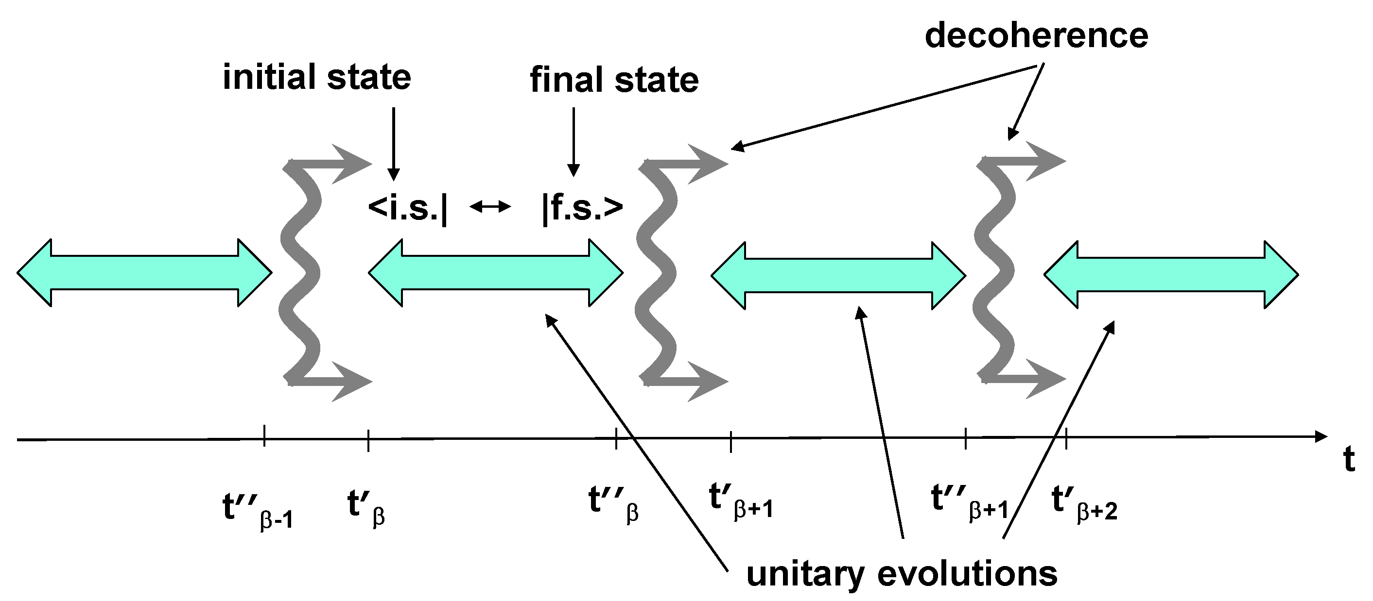
2. Chain of Unitary and Decoherence Events

The effect of decoherence is profound and, as demonstrated for the Pauli master equation, the presumed direction of decoherence ultimately controls the thermodynamic direction of time [8]. The present work extends these ideas to particle systems. The systems considered here experience two type of events: statistical, which can increase the phase volume occupied by the system, and quantum mechanical, which predict reversible (unitary) evolution of subsystems. Following the previous work [8], which is based on the approach developed by Pauli [10], unitary evolutions ${\mathfrak{U}}_{\beta }$ and decoherence events ${\mathfrak{D}}_{\beta }$ are presumed to occur as a chain $...,{\mathfrak{U}}_{\beta },{\mathfrak{D}}_{\beta },{\mathfrak{U}}_{\beta +1},{\mathfrak{D}}_{\beta +1},...$, separated by the time moments $...,t_{\beta }^{\prime },t_{\beta }^{″},t_{\beta +1}^{\prime },t_{\beta +1}^{″},...$ as illustrated in Figure 1. The events ${\mathfrak{U}}_{\beta }$ are reversible and entropy-preserving, while randomness and temporal directionality are introduced by events ${\mathfrak{D}}_{\beta }$, which add uncertainty and, ultimately, increase entropy of the system. This chain division of complex interactions is, of course, an idealisation of the physical reality but it is needed to separate and distinguish the influences of ${\mathfrak{U}}_{\beta }$ and ${\mathfrak{D}}_{\beta }$ and make the problem tractable. Such idealisations, however, are common in quantum mechanics: for example, separating unitary evolutions and non-unitary measurements. In reality, decoherence is likely to be a combined effect of tiny decohering violations of unitary mechanics combined with some unitary interactions (intrinsic or environmental). In this work, we tend to bypass the complex problem of the physical mechanism of decoherence and focus on its effect.

The question of quantum reality is complicated but, in the context of the present work, quantum events are connected to perceivable reality only through the initial $\left|i,t_{\beta }^{\prime }\right.〉$ and final states $\left|f,t_{\beta }^{″}\right.〉$; everything else in relation to the trajectories remains unknown and may be subject to different physical interpretations (we can refer to two-state quantum mechanics [22,23,24] as one of these interpretational possibilities). Superposition of all these trajectories contribute to the Feynman path integral which determines the statistical weights of the events. Each unitary event has its statistical weight $W_i^f$ defined by $W_i^f={\left|{\widehat{S}}_i^f\right|}^2$ where ${\widehat{S}}_i^f=〈f\left|\mathbb{U}\right({\tau }_{\beta }\left)\right|i〉$ is the scattering matrix, $\mathbb{U}\left({\tau }_{\beta }\right)$ reflects unitary evolution over period ${\tau }_{\beta }=t_{\beta }^{″}-t_{\beta }^{\prime }.$ For thermodynamic considerations, the Ŝ-matrix is assumed to be close to the unit matrix: $\widehat{\mathbf{S}}=\mathbf{I}+i\mathbf{h}$ and $∥\mathbf{h}∥\ll ∥\mathbf{I}∥$. Under these conditions, $\mathbf{h}$ must be Hermitian as long as $\widehat{\mathbf{S}}$ is unitary: $\mathbf{I}={\widehat{\mathbf{S}}}^{†}\widehat{\mathbf{S}}=\mathbf{I}+i(\mathbf{h}-{\mathbf{h}}^{†})+...$ The matrix $\mathbf{W}$ is then symmetric

$$W_i^f=W_f^i$$

(1)

which is important for thermodynamic consistency [8]. The smallness of $\mathbf{h}$ implies that the decoherence events are sufficiently frequent but, as discussed below, not excessively frequent. Note that some of the events $\left|i\right.〉$ $⟶\left|f\right.〉$ might be physically impossible (say, a transition violating a conservation law); in this case $W_i^f=W_f^i=0$.

Evaluation of the scattering matrix using quantum perturbation techniques have been repeatedly discussed in publications in general [10,25,26] and specifically in application to interactions of radiation and matter [27,28,29,30,31,32,33]. In these theories, the system Hamiltonian $\mathbb{H}$ is represented by a sum of the undisturbed component ${\mathbb{H}}_0$ and interaction component ${\mathbb{H}}_1$ so that $\mathbb{H}={\mathbb{H}}_0+{\mathbb{H}}_1$ with different corresponding characteristic times ${\tau }_0\sim 1/\left|{\mathbb{H}}_0\right|\ll {\tau }_1\sim 1/\left|{\mathbb{H}}_1\right|$ associated with these components. The characteristic time ${\tau }_{\beta }$ between the decoherence events is presumed to satisfy ${\tau }_0\ll {\tau }_{\beta }\ll {\tau }_1$ (see Reference [8]): condition ${\tau }_{\beta }\ll {\tau }_1$ is required for thermodynamic consistency (1), while condition ${\tau }_0\ll {\tau }_{\beta }$ enforces the conservation of energy in quantum transitions and eliminates the quantum Zeno effect. When evaluating the interaction Hamiltonian, atoms are commonly represented at the leading order by electric dipoles since the wavelength of radiated light significantly exceeds the typical size of the atoms.

Figure 1 illustrates a conventional (symmetric) case when decoherence occurs only in one temporal direction. The present work, however, allows for another possibility, which represents decoherence occurring backward in time—this process is called here recoherence (although term “recoherence” can have different interpretations elsewhere). In accordance with antisymmetric thermodynamics, recoherence is expected to be dominant for antimatter, while matter is dominated by decoherence. The symmetric version of thermodynamics corresponds to the same predominant direction of decoherence for both matter and antimatter.

The analysis of symmetric and antisymmetric master equations [8] indicate that, for any selected segment of unitary evolution ${\mathfrak{U}}_{\beta },$ the conversion rates are determined by the amplitudes of decohered components, whose presence depends on the directional properties of the decohering events ${\mathfrak{D}}_{\beta }$. There is, however, another constraint, which is linked to the presence of the recohered components. In simple terms, the recohered components of a reaction do not affect the probabilities and the rates of conversion as long as they can be present without violating any physical conservation laws. Depending on temporal direction of the kinetics rate equations, this constraint may or may not be satisfied automatically. Practically, this constraint terminates the conversions when the boundaries of physically possible values of the parameters are reached (e.g., concentrations of the components must be non-negative). The understanding offered by the analysis of Reference [8] can be summarised in the following proposition:

Proposition 1.

In decohering systems, the conversion rate is proportional to the probability amplitudes of the decohered components and, generally, is also constrained by the presence of the required recohered components (although the probability amplitudes of recohered components do not affect the conversion rate). Decohered (recohered) components are understood as properties of components immediately preceding or immediately following the segments of unitary interaction, irrespective of the temporal direction of decoherence (recoherence).

There are, however, some features that distinguish present consideration from the previous analysis [8] (where thermalisation was derived and not presumed). As discussed in Appendix A, the system considered here is assumed to be in a thermodynamic state, i.e., close to maximally mixed conditions (although not necessarily exactly in maximally mixed conditions, since this would imply achieving a thermodynamic equilibrium for an isolated system). This assumption allows us to treat two-particle states as separable (statistically independent), which is used in the further analysis.

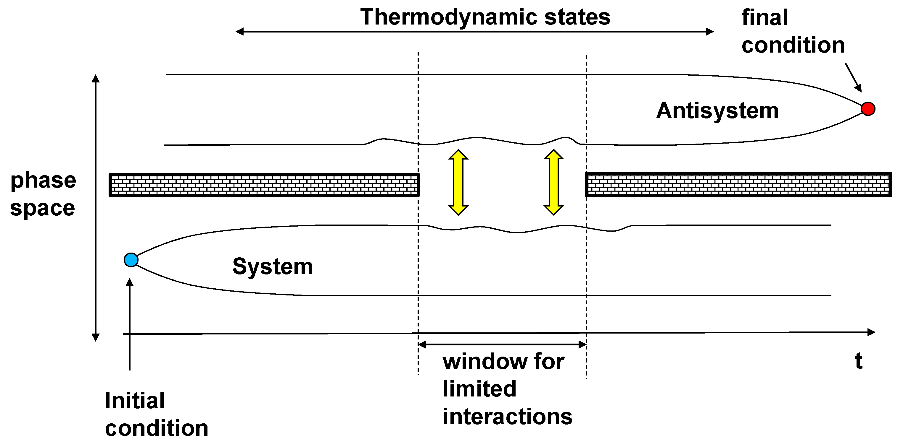
3. Kinetics and Thermodynamics of Indirect Interactions of Matter and Antimatter

This section investigates kinetics and thermodynamics of relatively weak interactions of matter and antimatter, when matter and antimatter are not in direct contact and not allowed to annihilate. This, however, does not prohibit a limited exchange of energy by virtual photons with energy $\Delta E$ as shown in Figure 2. The matter and antimatter are represented by atoms A and by antiatoms Ā that correspondingly belong to a thermodynamic system and antisystem (i.e., a system made of antimatter). Each of the atoms and antiatoms can be in excited or ground state and each of these states is not degenerate. The system under consideration is constrained by having only two energy states, since these relatively simple systems provide the best illustration for interactions of thermodynamics and kinetics. The excited state may also be referred to as the “roof state” to emphasise that this state corresponds to the highest possible energy in the system.

The numbers of atoms conserve the amounts of matter and antimatter

$$F_{{\mathrm{A}}^{*}}+F_{{\mathrm{A}}^{\circ }}=F_{\mathrm{A}}=\mathrm{const}\mathrm{and}{F}_{{\mathsf{Ā}}^{*}}+F_{{\mathsf{Ā}}^{\circ }}=F_{\mathsf{Ā}}=\mathrm{const}$$

(2)

and the energy

$$F_{{\mathrm{A}}^{\circ }}+F_{{\mathsf{Ā}}^{\circ }}=F^{\circ }=\mathrm{const}\mathrm{and}{F}_{{\mathrm{A}}^{*}}+F_{{\mathsf{Ā}}^{*}}=F^{*}=\mathrm{const}$$

(3)

The energy exchange reactions

$$\left(1\right){\mathrm{A}}^{*}+{\mathsf{Ā}}^{\circ }⟶{\mathrm{A}}^{\circ }+{\mathsf{Ā}}^{*}$$

(4)

$$\left(2\right){\mathrm{A}}^{\circ }+{\mathsf{Ā}}^{*}⟶{\mathrm{A}}^{*}+{\mathsf{Ā}}^{\circ }$$

(5)

are shown in Figure 2 and involve an energy transition through a virtual photon (the first reaction is on left-hand side, and the second is on right-hand side). The reaction rate constants are the same for forward and reverse reactions due to thermodynamic consistency (1) (or due to CP-invariance of quantum interaction Hamiltonians). The change in particle numbers due to reactions over the intervals $[t_{\beta }^{\prime },t_{\beta }^{″}]$ is given by

$$\Delta F_{\mathrm{A}{}^{\circ }}=F_{\mathrm{A}{}^{\circ }}+\Delta F,\Delta F_{{\mathrm{A}}^{*}}=F_{{\mathrm{A}}^{*}}-\Delta F,\Delta F_{\mathsf{Ā}{}^{\circ }}=F_{\mathsf{Ā}{}^{\circ }}-\Delta F,\Delta F_{{\mathsf{Ā}}^{*}}=F_{{\mathsf{Ā}}^{*}}+\Delta F$$

(6)

where $\Delta F=\Delta F_1-\Delta F_2$ is the effect of both reactions (4) and (5).

While the number of the energy states is limited to two, the atoms and antiatoms can be found in N secondary quantum states $J=1,...,N$, which do not affect the energy but reflect uncertainty present in any thermodynamic system. The value N is presumed to be very large (compared to the number of particles, which is also large) allowing us the use of classical statistics. Hence, $f_{\mathrm{X}}=F_{\mathrm{X}}/N\ll 1$ for any X = A${}^{\circ },$ A${}^{*},$ Ā${}^{\circ }$ or Ā${}^{*}$.

The overall system states form a Hilbert space of very large dimension, which can be estimated by $n_0\sim N^{F_{\mathrm{A}}+F_{\mathsf{Ā}}}/(F_{\mathrm{A}}!F_{\mathsf{Ā}}!)$, but such description would be excessively detailed and is not needed. Energy exchange occurs only between atom/antiatom pairs— interactions between three and more particles are unlikely and can be neglected. Hence, only two-particle states need to be considered, which generally correspond to every one of the $F_{\mathrm{A}}{F}_{\mathsf{Ā}}$ possible pairs distributed over the $N^2$ possible states $J_{\mathrm{A}},J_{\mathsf{Ā}}=1,...,N$. The system is assumed to be close to a maximally mixed state with respect to the secondary states implying that $F_{\mathrm{A}}{F}_{\mathsf{Ā}}$ pairs are uniformly distributed between $N^2$ quantum states (see Appendix A). In this case, the probability of a selected two-particle state being occupied by an atom A and an antiatom Ā is given by $P=f_{\mathrm{A}}{f}_{\mathsf{Ā}}$. The energy states, however, are not necessarily at equilibrium and the system can evolve.

The probability of reactions (4) and (5) is determined by statistical weights $w=W_{*\circ }^{\circ *}=W_{\circ *}^{*\circ },$ where $W_{ab}^{ba}={\left|{\widehat{S}}_{ab}^{ba}\right|}^2$, and ${\widehat{S}}_{ab}^{ba}=〈{\mathrm{A}}^b+{\mathsf{Ā}}^a\left|\mathbb{U}\left({\tau }_{\beta }\right)\right|{\mathrm{A}}^a+{\mathsf{Ā}}^b〉$, while a and b denote “*” or “∘”. Many of the elements of matrix $\mathbf{W}$ are zeros since they correspond to impossible events. For example, $W_{**}^{\circ *}=0$ corresponds to reaction A${}^{*}+$ Ā${}^{*}⟶$ A${}^{\circ }+$ Ā${}^{*}$ that violates conservation of energy. Generally, w can depend on secondary sates $J_{\mathrm{A}}$ and $J_{\mathsf{Ā}}$ or even imply a transition between secondary states $\left|ab,J_{\mathrm{A}}^{\prime }{J}_{\mathsf{Ā}}^{\prime },t=t^{\prime }\right.〉⟶\left|ba,J_{\mathrm{A}}^{″}{J}_{\mathsf{Ā}}^{″},t=t^{″}\right.〉$—this does not affect the structure of the final equations since we are interested only in following the energy states. Note that the majority of two-particle states are not occupied since $F_{\mathrm{X}}\ll N,$ that $w\ll 1$ and that $w=0$ for the most of $\mathbf{J}=(J_{\mathrm{A}}^{\prime },J_{\mathsf{Ā}}^{\prime },J_{\mathrm{A}}^{″},J_{\mathsf{Ā}}^{″})$; hence the expected number of conversion events is relatively small $\Delta F\ll F_{\mathrm{X}}$.

The probability amplitudes for energy transfer between atoms by a virtual photon can be evaluated for specific conditions of the interactions. Assuming that two free atoms are located at the distance $r,$ the probability amplitudes have been repeatedly evaluated by quantum perturbation techniques [31,33]. Unlike real photons, the virtual photons are allowed to violate the four-momentum expression for massless particles and, perhaps, represent more a mathematical perturbation term than a real physical object. The perturbation theories [31,33] use the dipole approximation and determine that, as the distance r increases, the virtual photon becomes more and more “real" while the strength of interaction scales as $r^{-6}$ in the near (radiationless) zone and as $r^{-2}$ in the far (radiational) zone. In general, both of these regimes are consistent with the consideration presented in this section. This consideration, however, necessarily requires that the photon (purely virtual in the near zone or quasi-real in the far zone) is in a jointly coherent state with the atoms, while the transition between the moment of emission and the moment of absorption depicted in Figure 2 remains unitary and is not affected by decoherence. This implies that the characteristic decoherence time is assumed to be longer that the characteristic life time of the quasi-real photons. Unlike the “real” photons considered in the following sections, the virtual photons illustrated by Figure 2 do not represent objects independently controlled by the laws of statistical physics. The atoms and antiatoms, however, decohere (or recohere) after interaction and thus become true statistical objects, as considered in the rest of this section.

3.1. Symmetric Kinetics

The case of symmetric decoherence, which corresponds to symmetric thermodynamics, is shown in Figure 2 (top). In this case, the decohered components are represented by reactants and the recohered components are represented by products. Hence, according to Proposition 1, the average number of convention events during the time interval $[t_{\beta }^{\prime },t_{\beta }^{″}]$ is given by

$$\Delta F_1=K_1{f}_{{\mathrm{A}}^{*}}^{\prime }{f}_{{\mathsf{Ā}}^{\circ }}^{\prime }H\left(f_{{\mathrm{A}}^{\circ }}^{″}\right)H\left(f_{{\mathsf{Ā}}^{*}}^{″}\right)$$

(7)

$$\Delta F_2=K_2{f}_{{\mathrm{A}}^{\circ }}^{\prime }{f}_{{\mathsf{Ā}}^{*}}^{\prime }H\left(f_{{\mathrm{A}}^{*}}^{″}\right)H\left(f_{{\mathsf{Ā}}^{\circ }}^{″}\right)$$

(8)

for reactions (4) and (5) correspondingly. Here, where $H\left(F\right)=1$ when $F>0$ and $H\left(F\right)=0$ when $F\le 0$ is the Heaviside step function, the “prime” superscript denotes parameters of the system at $t=t_{\beta }^{\prime }$ and “double prime” at $t=t_{\beta }^{″}$. The reaction rate is determined by the magnitudes of the decohered components ($f_{{\mathrm{A}}^{*}}^{\prime }$ and $f_{{\mathsf{Ā}}^{\circ }}^{\prime }$ for the first reaction), which, as discussed in Appendix A, are deemed to be stochastically independent, and constrained by the presence of recohered components ($f_{{\mathrm{A}}^{\circ }}^{″},f_{{\mathsf{Ā}}^{*}}^{″}>0$ for the first reaction). The reaction constants are given by

$$K_1=\sum _{\mathbf{J}}{W}_{*\circ }^{\circ *}\left(\mathbf{J}\right)=\sum _{\mathbf{J}}{W}_{\circ *}^{*\circ }\left(\mathbf{J}\right)=K_2$$

(9)

irrespective whether the reactions affect the secondary states or not.

The difference between particle numbers before and after the reaction can often be neglected, that is $F_{\mathrm{X}}^{″}\approx F_{\mathrm{X}}^{\prime }\approx F_{\mathrm{X}}$ and $f_{\mathrm{X}}^{″}\approx f_{\mathrm{X}}^{\prime }\approx f_{\mathrm{X}}$ for all X since all $F_{\mathrm{X}}$ are much larger then $1.$ Each reaction occurrence can change the numbers of particles only by 1. Given a reaction occurring in a particular box, the overall change in particle numbers at a given time step is relatively low $1+\left|\Delta F\right|\ll F_{\mathrm{X}}$. This leads us to possibility of converting Equations (6)–(8) into an ordinary differential equation (ODE), which is often called the reaction kinetics equation. While, generally, this conversion may depend on whether the reaction rate equation is to be solved forward in time (with initial conditions) or backward in time (with final conditions), the forward-time and backward-time ODEs are equivalent in this case. With $\Delta F=\Delta F_1-\Delta F_2$ in (6), the reaction rate equation take the form

$$\begin{array}{cc}\hfill -\frac{d{f}_{{\mathrm{A}}^{*}}}{dt}& =-\frac{d{f}_{{\mathsf{Ā}}^{\circ }}}{dt}=\frac{d{f}_{{\mathrm{A}}^{\circ }}}{dt}=\frac{d{f}_{{\mathsf{Ā}}^{*}}}{dt}\hfill \\ & =k_{\tau }\left(f_{{\mathrm{A}}^{*}}{f}_{{\mathsf{Ā}}^{\circ }}H\left(f_{{\mathrm{A}}^{\circ }}\right)H\left(f_{{\mathsf{Ā}}^{*}}\right)-f_{{\mathrm{A}}^{\circ }}{f}_{{\mathsf{Ā}}^{*}}H\left(f_{{\mathrm{A}}^{*}}\right)H\left(f_{{\mathsf{Ā}}^{\circ }}\right)\right)\hfill \\ & \underset{t\uparrow }{=}{k}_{\tau }\left(f_{{\mathrm{A}}^{*}}{f}_{{\mathsf{Ā}}^{\circ }}-f_{{\mathrm{A}}^{\circ }}{f}_{{\mathsf{Ā}}^{*}}\right)\hfill \end{array}$$

(10)

where $k_{\tau }=K_1/\tau =K_2/\tau$, $\tau =t_{\beta +1}-t_{\beta }$. For the forward-time equation, the Heaviside functions can be omitted since all populations F remain non-negative as long as the initial conditions are also non-negative. The Heaviside functions are nevertheless needed if Equation (10) is to be solved backward in time. Equation (10) is CP-invariant and is not affected by swapping A and Ā.

Note that the Gibbs distribution with any temperature T

$$\frac{f_{{\mathrm{A}}^{*}}^{\left(e\right)}}{f_{{\mathrm{A}}^{\circ }}^{\left(e\right)}}=\frac{f_{{\mathsf{Ā}}^{*}}^{\left(e\right)}}{f_{{\mathsf{Ā}}^{\circ }}^{\left(e\right)}}=\exp \left(-\frac{\Delta E}{T}\right)$$

(11)

represents an equilibrium ($d/dt=0$) solution for Equation (10). The superscript “$\left(e\right)$” is used to indicate values related to equilibrium. The thermodynamic ground state $(f_{{\mathrm{A}}^{*}}^{\left(e\right)}/f_{{\mathrm{A}}^{\circ }}^{\left(e\right)}=0$) corresponds to the coldest possible temperature $T=+0$ and the thermodynamic roof state $(f_{{\mathrm{A}}^{\circ }}^{\left(e\right)}/f_{{\mathrm{A}}^{*}}^{\left(e\right)}=0$) corresponds to the hottest possible temperature $T=-0$. Note that, in systems with a finite number of energy levels, the temperatures can be negative and that negative temperatures are hotter than positive temperatures ([34,35,36]).

The conservation laws (2) and (3) in conjunction with equilibrium condition (11) uniquely determine the equilibrium state by

$$\frac{f_{{\mathrm{A}}^{\circ }}^{\left(e\right)}}{f_{\mathrm{A}}}=\frac{f_{{\mathsf{Ā}}^{\circ }}^{\left(e\right)}}{f_{\mathsf{Ā}}}=\frac{f^{\circ }}{f_{\mathrm{A}}+f_{\mathsf{Ā}}}\mathrm{and}\frac{f_{{\mathrm{A}}^{*}}^{\left(e\right)}}{f_{\mathrm{A}}}=\frac{f_{{\mathsf{Ā}}^{*}}^{\left(e\right)}}{f_{\mathsf{Ā}}}=\frac{f^{*}}{f_{\mathrm{A}}+f_{\mathsf{Ā}}}$$

(12)

In this case T is not fixed and is determined by (11). With the use of conservation laws (2) and (3), the symmetric kinetics rate equation specified by (10) can be rewritten in the form

$$\frac{d{f}_{{\mathrm{A}}^{\circ }}}{dt}=k_{\tau }\left(f_{\mathrm{A}}+f_{\mathsf{Ā}}\right)\left(f_{{\mathrm{A}}^{\circ }}^{\left(e\right)}-f_{{\mathrm{A}}^{\circ }}\right)$$

(13)

It is clear that the system always converges to the equilibrium and that this equilibrium is stable.

3.2. Antisymmetric Kinetics

The case shown at the bottom of Figure 2 corresponds to antisymmetric decoherence and thermodynamics. Note that the model under consideration is invariant with respect to swapping A and Ā and changing t to $-t$. As the particles proceed from the past to the future, the atoms A are subject to decoherence events (which impose probability constraints after decoherence), while the antiatoms Ā are subject to the recoherence events (which impose the probability constraints before recoherence). According to Proposition 1, this leads to the following expressions for the average number of (4) and (5) reaction events

$$\Delta F_1=K_1{f}_{{\mathrm{A}}^{*}}^{\prime }{f}_{{\mathsf{Ā}}^{*}}^{″}H\left(f_{{\mathrm{A}}^{\circ }}^{″}\right)H\left(f_{{\mathsf{Ā}}^{\circ }}^{\prime }\right)$$

(14)

$$\Delta F_2=K_2{f}_{{\mathrm{A}}^{\circ }}^{\prime }{f}_{{\mathsf{Ā}}^{\circ }}^{″}H\left(f_{{\mathrm{A}}^{*}}^{″}\right)H\left(f_{{\mathsf{Ā}}^{*}}^{\prime }\right)$$

(15)

where $K_1=K_2=K$ are still defined by (9). The reaction rate of the first reaction is determined by decohered components $f_{{\mathrm{A}}^{*}}^{\prime }$ and $f_{{\mathsf{Ā}}^{*}}^{″}$ and constrained by the presence of recohered components $f_{{\mathrm{A}}^{\circ }}^{″},f_{{\mathsf{Ā}}^{\circ }}^{\prime }>0$.

As previously, the conversion of these relations into ODE, assuming $F_{\mathrm{X}}\gg 1$ for all X and $k_{\tau }=K_1/\tau =K_2/\tau$, results in the following reaction rate equation

$$\begin{array}{cc}\hfill -\frac{d{f}_{{\mathrm{A}}^{*}}}{dt}& =-\frac{d{f}_{{\mathsf{Ā}}^{\circ }}}{dt}=\frac{d{f}_{{\mathrm{A}}^{\circ }}}{dt}=\frac{d{f}_{{\mathsf{Ā}}^{*}}}{dt}\hfill \\ & =k_{\tau }\left(f_{{\mathrm{A}}^{*}}{f}_{{\mathsf{Ā}}^{*}}H\left(f_{{\mathrm{A}}^{\circ }}\right)H\left(f_{{\mathsf{Ā}}^{\circ }}\right)-f_{{\mathrm{A}}^{\circ }}{f}_{{\mathsf{Ā}}^{\circ }}H\left(f_{{\mathrm{A}}^{*}}\right)H\left(f_{{\mathsf{Ā}}^{*}}\right)\right)\hfill \\ & \underset{f_{\mathrm{X}}>0}{=}{k}_{\tau }\left(f_{{\mathrm{A}}^{*}}{f}_{{\mathsf{Ā}}^{*}}-f_{{\mathrm{A}}^{\circ }}{f}_{{\mathsf{Ā}}^{\circ }}\right)\hfill \end{array}$$

(16)

Here, we neglect the difference between $f^{\prime }$ and $f^{″}$ since the change brought by each the reaction event is relatively small. The Heaviside functions can be omitted for simplicity but the reactions need to be terminated if any of the components is exhausted. The derived equation is CPT-invariant: swapping A and Ā and substituting $-t$ for t does not change Equation (16).

Note that the Gibbs distribution with two intrinsic temperatures: T for matter and $\overline{T}$ for antimatter

$$\frac{f_{{\mathrm{A}}^{*}}^{\left(e\right)}}{f_{{\mathrm{A}}^{\circ }}^{\left(e\right)}}=\exp \left(-\frac{\Delta E}{T}\right),\frac{f_{{\mathsf{Ā}}^{*}}^{\left(e\right)}}{f_{{\mathsf{Ā}}^{\circ }}^{\left(e\right)}}=\exp \left(-\frac{\Delta E}{\overline{T}}\right),T=-\overline{T}$$

(17)

corresponds to the equilibrium state ($d/dt=0$) of Equation (16). The conservation laws specified by (2) and (3) require that equilibrium states are compliant with

$$\frac{f_{{\mathrm{A}}^{\circ }}^{\left(e\right)}}{f_{\mathrm{A}}}=\frac{f_{{\mathsf{Ā}}^{*}}^{\left(e\right)}}{f_{\mathsf{Ā}}}=\frac{f_{\mathsf{Ā}}-f^{\circ }}{f_{\mathsf{Ā}}-f_{\mathrm{A}}}\mathrm{and}\frac{f_{{\mathrm{A}}^{*}}^{\left(e\right)}}{f_{\mathrm{A}}}=\frac{f_{{\mathsf{Ā}}^{\circ }}^{\left(e\right)}}{f_{\mathsf{Ā}}}=\frac{f^{\circ }-f_{\mathrm{A}}}{f_{\mathsf{Ā}}-f_{\mathrm{A}}}$$

(18)

Note that physical equilibrium states exists only when both $f^{\circ }$ and $f^{*}$ have values between $f_{\mathsf{Ā}}$ and $f_{\mathrm{A}}$. The conservation laws (2) and (3) transform (16) into

$$\frac{d{f}_{{\mathrm{A}}^{\circ }}}{dt}=k_{\tau }\left(f_{\mathsf{Ā}}-f_{\mathrm{A}}\right)\left(f_{{\mathrm{A}}^{\circ }}^{\left(e\right)}-f_{{\mathrm{A}}^{\circ }}\right)$$

(19)

where $f_{{\mathrm{A}}^{\circ }}^{\left(e\right)}$ is formally defined by (18) irrespective of existence of a physical equilibrium state. The equation is stable only if $f_{\mathsf{Ā}}>f_{\mathrm{A}}$. If a physical equilibrium does not exist or exists but is unstable, evolution of Equation (19) is terminated when at least one of the population numbers $f_{{\mathrm{A}}^{*}}$, $f_{{\mathrm{A}}^{\circ }}$, $f_{{\mathsf{Ā}}^{*}}$ or $f_{{\mathsf{Ā}}^{\circ }}$ becomes zero.

3.3. Properties of Antisymmetric Kinetics

The properties of the antisymmetric kinetics are examined below for three characteristic cases $f_{\mathsf{Ā}}=f_{\mathrm{A}}$, $f_{\mathsf{Ā}}\gg f_{\mathrm{A}}$ and $f_{\mathsf{Ā}}\ll f_{\mathrm{A}},$ which are nominally labelled “early universe”, “travelling to antiworld” and “experiment with antimatter”. Practically, only the last case may be related to realistic experiments or observations in present conditions.

• Early universe: $f_{\mathsf{Ā}}=f_{\mathrm{A}}$. Equilibrium under conditions of having the same amounts of matter and antimatter, which is specified by $f_{{\mathrm{A}}^{\circ }}=$ $f_{{\mathsf{Ā}}^{*}}$ and $f_{{\mathrm{A}}^{*}}=$ $f_{{\mathsf{Ā}}^{\circ }}$, is neutral and can be achieved at different temperatures $T=-\overline{T}$ but is subject to the additional condition $f_{{\mathsf{Ā}}^{*}}+f_{{\mathrm{A}}^{*}}=$ $f_{{\mathsf{Ā}}^{\circ }}+$ $f_{{\mathrm{A}}^{\circ }}$, which must be satisfied in compliance with the solution $f_{{\mathrm{A}}^{\circ }}=$ $f_{{\mathsf{Ā}}^{*}}=$ $f_{{\mathrm{A}}^{*}}=$ $f_{{\mathsf{Ā}}^{\circ }}$ that has infinite temperature $1/T=1/\overline{T}=0$.
• Travelling to antiworld: $f_{\mathsf{Ā}}\gg f_{\mathrm{A}}$. A matter traveller of a small mass travels to an antiworld populated by large amounts of antimatter (or the traveller is a fictional Time Lord and somehow manages to turn his world line back in our world time). This case has a stable thermodynamic equilibrium. Assuming that the intrinsic temperature of antiworld is positive $\overline{T}>0$ this equilibrium can be achieved only at negative temperatures $T=-\overline{T}$ of the traveller. Practically this means that the traveller would be burned.
• Experiment with antimatter: $f_{\mathsf{Ā}}\ll f_{\mathrm{A}}$. In this case equilibrium between matter and antimatter is unstable and practically impossible. Depending on initial conditions, the antimatter object would fall into the intrinsic ground state (apparent roof state) or, possibly but much less likely, into the intrinsic roof state (apparent ground state).

These conclusions are based on kinetics rate equations but are in general agreement with previous analysis of interactions matter and antimatter based on thermodynamics. Note that the apparent heat capacity of antimatter is negative in antisymmetric thermodynamics [7]. A brief summary of thermodynamic behaviour for negative temperatures and negative heat capacities can be found in Reference [36] and many other publications. It must be mentioned that unlike in previous works, matter/antimatter annihilations and baryon number violations are not allowed here, while matter and antimatter interact only by exchange of radiation. The main results of the antisymmetric treatment of the problem are summarised by this proposition:

Proposition 2.

The antisymmetric (CPT-invariant) extension of thermodynamics and kinetics from matter to antimatter corresponds to decoherence being dominant for matter and recoherence being dominant for antimatter. Under these conditions, thermodynamic equilibrium between matter and antimatter is theoretically possible but practically unlikely since this requires negative intrinsic temperatures. In most cases, a thermodynamic antisystem should fall into one of its extreme states, most likely the intrinsic ground state.

3.4. H-Theorems for Symmetric and Antisymmetric Kinetics

The intrinsic entropy for each component is defined conventionally

$$S_{\mathrm{X}}=-F_{{\mathrm{X}}^{\circ }}\ln \left(f_{{\mathrm{X}}^{\circ }}\right)-F_{{\mathrm{X}}^{*}}\ln \left(f_{{\mathrm{X}}^{*}}\right),\mathrm{X}=\mathrm{A},\mathrm{Ā}$$

(20)

The kinetics considered in this section are compliant with the H-theorems as formulated in the following proposition.

Proposition 3.

The symmetric $S_s=S_{\mathrm{A}}+S_{\mathsf{Ā}}$ and antisymmetric $S_a=S_{\mathrm{A}}-S_{\mathsf{Ā}}$ entropies are increased forward in time t by symmetric and antisymmetric kinetics correspondingly until the system evolution reaches its equilibrium or is terminated by physical constraints.

The entropy-increasing properties of conventional symmetric kinetics are well-known—the treatment of the antisymmetric case is shown below. We use the indicator ${\mathsf{\Theta }}_{\mathrm{X}}$ that is defined ${\mathsf{\Theta }}_{\mathrm{X}}=1$ for X = A${}^{\circ },$ A${}^{*}$ and ${\mathsf{\Theta }}_{\mathrm{X}}=-1$ for X = Ā${}^{\circ },$ Ā${}^{*}$ and conclude:

$$\frac{d{S}_a}{dt}=-\sum _{\mathrm{X}}{\mathsf{\Theta }}_{\mathrm{X}}\frac{d{F}_{\mathrm{X}}}{dt}\left(\ln \left(f_{\mathrm{X}}\right)+1\right)=k_{\tau }\left(f_{{\mathrm{A}}^{*}}{f}_{{\mathsf{Ā}}^{*}}-f_{{\mathrm{A}}^{\circ }}{f}_{{\mathsf{Ā}}^{\circ }}\right)\ln \left(\frac{f_{{\mathrm{A}}^{*}}{f}_{{\mathsf{Ā}}^{*}}}{f_{{\mathrm{A}}^{\circ }}{f}_{{\mathsf{Ā}}^{\circ }}}\right)\ge 0$$

(21)

for any $f_{{\mathrm{A}}^{*}},$ $f_{{\mathsf{Ā}}^{*}},$ $f_{{\mathrm{A}}^{\circ }}$ and $f_{{\mathsf{Ā}}^{\circ }}$.

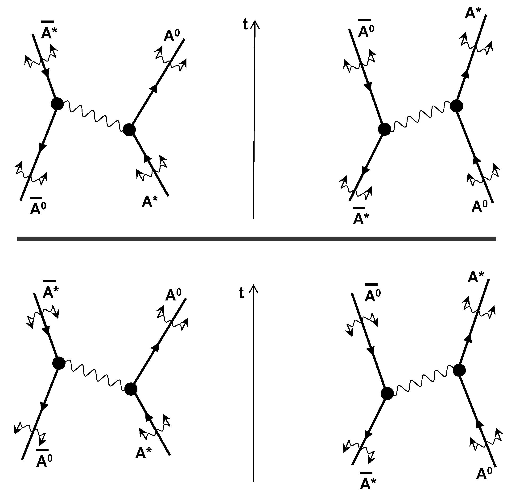
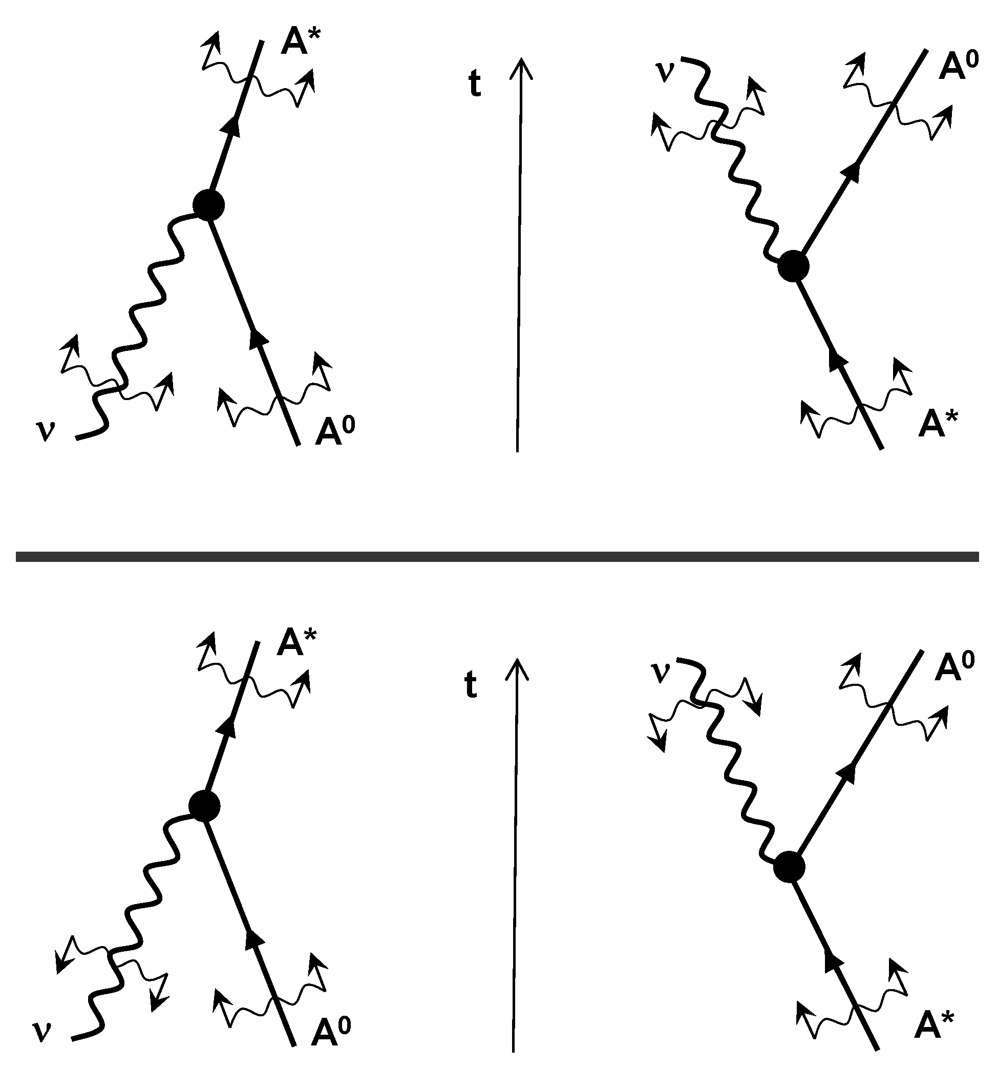
4. Interactions of Radiation and Matter

In this section we consider interactions of radiation with matter, assuming different decohering properties of radiation. Interactions of a single quantum state populated by q photons (which are bosons and do not restrict q) with $F_{\mathrm{A}}$ matter atoms specified by (1) absorption and (2) emission reaction equations

$$\left(1\right){\mathrm{A}}^{\circ }+\nu ⟶{\mathrm{A}}^{*}\mathrm{and}\left(2\right){\mathrm{A}}^{*}⟶{\mathrm{A}}^{\circ }+\nu$$

(22)

The probability amplitudes of absorption and emission have been extensively studied in the literature [28,29,30,32] and are consistent with the emission/absorption probability amplitudes evaluated for quasi-real photons [33]. Unlike virtual and quasi-real photons of the previous section, the photons and atoms considered here can decohere (or recohere) and, thus, are both subject to the laws of statistical physics. Note that photon populations q can be both small and large, depending on conditions. Assuming atom population per secondary state $f_{{\mathrm{A}}^a}=F_{{\mathrm{A}}^a}/N$ is at equilibrium, the canonical distribution is linked to the temperature by

$$\frac{f_{{\mathrm{A}}^{*}}}{f_{{\mathrm{A}}^{\circ }}}=\exp \left(-\frac{\Delta E}{T}\right)$$

(23)

4.1. Radiation with Prevailing Decoherence

In this subsection we assume that radiation has the same decohering properties as matter, which is illustrated in Figure 3 (top). The single and double primes are used to relate the values before and after each reaction: there are $q^{\prime }$ photons before and $q^{″}$ after the reaction, as well as $F_{{\mathrm{A}}^{\circ }}^{\prime }$ and $F_{{\mathrm{A}}^{\circ }}^{″}$ atoms before and after reactions in the ground state and $F_{{\mathrm{A}}^{*}}^{\prime }$ and $F_{{\mathrm{A}}^{*}}^{″}$ atoms before and after reaction in the excited state. Note that $q^{″}=q^{\prime }-1$ for the absorption reaction and $q^{″}=q^{\prime }+1$ for the emission reaction. The absorption reaction is considered first. As shown in Figure 3 (top), all particles (atoms and photons) decohere before and after the reactions. According to Proposition 1, the number of reactions per reaction time $\tau$ is given by

$$\Delta q_1=K{f}_{{\mathrm{A}}^{\circ }}^{\prime }{q}^{\prime }H\left(f_{{\mathrm{A}}^{*}}^{″}\right)\mathrm{and}\Delta q_2=K{f}_{{\mathrm{A}}^{*}}^{\prime }H\left(f_{{\mathrm{A}}^{\circ }}^{″}\right)H\left(q^{″}\right)$$

(24)

for the absorption and emission reaction correspondingly with K being the reaction constant and the overall effect on photon population given by $\Delta q=\Delta q_2-\Delta q_1$. Since q can be small, the differences between $q^{\prime }$ and $q^{″}$ cannot generally be neglected, although assuming $f_{{\mathrm{A}}^a}^{″}=F_{{\mathrm{A}}^a}^{″}/N\approx F_{{\mathrm{A}}^a}^{\prime }/N=f_{{\mathrm{A}}^a}^{\prime }$ is still acceptable since $F_{{\mathrm{A}}^a}\gg 1$. Conversion of these relations into ODEs is similar to the previous considerations but there is one point that needs clarification. We seek to obtain a forward-time kinetics rate equation as this equation is useful for us, since in the real world we set the initial (and not final) conditions. This means that we can specify $q^{\prime }$ but not $q^{″}$, and must identify the current value of the population q with $q^{\prime }$ and put $q^{″}=q+1$ for the emission reaction. This results in

$$\frac{dq}{dt}=k{f}_{{\mathrm{A}}^{*}}H\left(f_{{\mathrm{A}}^{\circ }}\right)H\left(q+1\right)-kq{f}_{{\mathrm{A}}^{\circ }}H\left(f_{{\mathrm{A}}^{*}}\right)$$

(25)

where $k=K/\tau$. The Heaviside constraints can be omitted. For example, $H\left(q+1\right)=1$ since $q+1$ is always positive. This equation is not consistent with the Einstein theory of radiation [27] and does not reproduce the Bose–Einstein statistics. Indeed assuming Gibbs distribution for atoms (23) we obtain for the equilibrium population

$$q^{\left(e\right)}=\frac{f_{{\mathrm{A}}^{*}}}{f_{{\mathrm{A}}^{\circ }}}=\exp \left(-\frac{\Delta E}{T}\right)$$

(26)

that is inconsistent with the expected physical behaviour of radiation since $q^{\left(e\right)}\to 1$ as $T\to \infty$.

4.2. Radiation with Prevailing Recoherence

In this subsection, radiation is presumed to predominantly recohere, while matter is still conventionally dominated by decoherence as shown in Figure 3 (bottom). In this case, the number of reactions per reaction time $\tau$ is given by

$$\Delta q_1=K{f}_{{\mathrm{A}}^{\circ }}^{\prime }H\left(f_{{\mathrm{A}}^{*}}^{″}\right)H\left(q^{\prime }\right)\mathrm{and}\Delta q_2=K{f}_{{\mathrm{A}}^{*}}^{\prime }{q}^{″}H\left(f_{{\mathrm{A}}^{\circ }}^{″}\right)$$

(27)

This equation is converted into ODE by assuming, as previously, that $q=q^{\prime },$ while taking into account that $q^{″}=q^{\prime }+1$ in the emission reaction. The equation takes the form

$$\frac{dq}{dt}=k(q+1)f_{{\mathrm{A}}^{*}}H\left(f_{{\mathrm{A}}^{\circ }}\right)-k{f}_{{\mathrm{A}}^{\circ }}H\left(f_{{\mathrm{A}}^{*}}\right)H\left(q\right)$$

(28)

The constraint $H\left(q\right)$ in the last term prevents q from becoming negative, while the other Heaviside functions in this equation can be omitted. With distribution (23) specified, the equilibrium distribution for this equation is given by

$$q^{\left(e\right)}=\frac{f_{{\mathrm{A}}^{\circ }}}{f_{{\mathrm{A}}^{*}}}-1=\exp \left(\frac{\Delta E}{T}\right)-1$$

(29)

which is obviously incorrect since $q^{\left(e\right)}\to 0$ as $T\to \infty$.

4.3. Decoherence-Neutral Radiation

The remaining option for radiation is to be decoherence-neutral, implying that neither decoherence nor recoherence can dominate unconditionally. Statistic nature of thermodynamic interactions, however, implies that interactions of photons and matter must involve some degree of decoherence. Decoherence-neutral interaction of photon with matter is depicted in Figure 4 (top). The atom decoheres both before and after emission or absorption, while the photon decoheres before absorption and recoheres after emission. The decohered states of the photon are caused not by intrinsic mechanisms pertaining to the electromagnetic fields but by interactions with matter. Under these conditions decoherence/recoherence of the photon in Figure 5 is effectively time-symmetric.

A possible physical scenario for decoherence-neutral radiation is that, initially, the q photons are in a coherent Fock state but they decohere due to weak decohering interactions with atoms (or antiatoms). The decohered photons are then engaged into stronger energy interactions with atoms, which can lead, although with a small probability, to absorption or emission of a photon. When all interactions with matter are completed, the remaining photons recohere back into a Fock state.

Absorption and emission of photons are now considered. There are $q^{\prime }$ photons before the reaction and $q^{″}$ after the reaction. According to the analysis of the previous sections, the number of reactions per reaction time $\tau$ is given by

$$\Delta q_1=K{f}_{{\mathrm{A}}^{\circ }}^{\prime }{q}^{\prime }H\left(f_{{\mathrm{A}}^{*}}^{″}\right)$$

(30)

for the absorption reaction, where $F_{{\mathrm{A}}^{*}}^{″}\approx F_{{\mathrm{A}}^{*}}^{\prime }$ and $q^{\prime }=q^{″}+1\ne q^{″}$ and

$$\Delta q_2=K{f}_{{\mathrm{A}}^{*}}^{\prime }{q}^{″}H\left(f_{{\mathrm{A}}^{\circ }}^{″}\right)$$

(31)

for the emission reaction, where $F_{{\mathrm{A}}^{\circ }}^{″}\approx F_{{\mathrm{A}}^{\circ }}^{\prime }$ and $q^{″}=q^{\prime }+1\ne q^{\prime }$. Since photon population q can be small, the differences between $q^{\prime }$ and $q^{″}$ cannot generally be neglected. Conversion of these relations into ODE is similar to the previous considerations. As we seek to obtain a forward-time reaction rate equation, the current value q should be identified with $q^{\prime }$ not $q^{″}$, since the contrary treatment may lead to contradictions. For example, if $q=0$ at $t=0$ and q is identified with $q^{″}$ then the first reaction must be emission with $q^{″}=q^{\prime }+1$. We can set $q^{\prime }=0$ but cannot assume $q^{″}=0$ since $q^{\prime }=q^{″}-1=q-1=-1<0$ at $t=0$, which is unphysical. With $q^{\prime }=q,$ the forward-time kinetics rate equation takes the form

$$\begin{array}{cc}\hfill \frac{dq}{dt}& =k(q+1)f_{{\mathrm{A}}^{*}}H\left(f_{{\mathrm{A}}^{\circ }}\right)-kq{f}_{{\mathrm{A}}^{\circ }}H\left(f_{{\mathrm{A}}^{*}}\right)\hfill \\ & =k(q+1)f_{{\mathrm{A}}^{*}}-kq{f}_{{\mathrm{A}}^{\circ }}=k\left(f_{{\mathrm{A}}^{*}}-q\left(f_{{\mathrm{A}}^{\circ }}-f_{{\mathrm{A}}^{*}}\right)\right)\hfill \end{array}$$

(32)

where $k=K/\tau$ and the Heaviside constraints are not needed here since Equation (32) is formulated for solving it forward in time. Equation (32) coincides with the Einstein theory of radiation [27]. The same result has been obtained in the quantum field theory [30] (due to pioneering work of Dirac [28]), effectively assuming coherent radiation in a Fock state $\left|q\right.〉$ and decohering matter. The photon creation and annihilation operators ${\widehat{a}}^{†}\left|q\right.〉={(q+1)}^{1/2}\left|q+1\right.〉$ and $\widehat{a}\left|q\right.〉={\left(q\right)}^{1/2}\left|q-1\right.〉$ have the probability amplitudes consistent with the creation and annihilation rates specified by (32). The quantum of energy associated with the photon is transferred into decohered state of matter during absorption and recoheres back into the Fock state during emission—this explanation matches the statistical interpretation given above, although decoherence and recoherence are not explicitly considered or discussed in the standard framework of second quantisation.

Assuming Gibbs distribution (23), where $\Delta E=h\nu ,$ the equilibrium solution is correctly given by the Bose-Einstein statistics [35]

$$q^{\left(e\right)}=\frac{1}{\exp \left(\frac{h\nu }{T}\right)-1}$$

(33)

If the overall energy is constant, this distribution maximises the entropy $S_{\nu }+S_{\mathrm{A}},$ where

$$S_{\nu }=\left(1+q\right)\ln \left(1+q\right)-q\ln \left(q\right)$$

(34)

and $S_{\mathrm{A}}$ is defined by (20). If many photon quantum states are present $i=1,2,...,N_q$ then Equation (32) needs to be written for population $q_{\left(i\right)}$ at every state

$$\frac{d{q}_{\left(i\right)}}{dt}=k(q_{\left(i\right)}+1)f_{{\mathrm{A}}^{*}}-k{q}_{\left(i\right)}{f}_{{\mathrm{A}}^{\circ }},i=1,...,N_q$$

(35)

Evaluating the sum $Q={\Sigma }_i{q}_{\left(i\right)}$ results in the common form of the Einstein equation

$$\frac{dQ}{dt}=k(Q+N_q)f_{{\mathrm{A}}^{*}}-kQ{f}_{{\mathrm{A}}^{\circ }}$$

(36)

Note that the stable equilibrium solution (33) exists only for positive temperatures T. For negative temperatures $T<0$ in (23), which corresponds to $f_{{\mathrm{A}}^{\circ }}<f_{{\mathrm{A}}^{*}}$ in (32), Equation (35) is unstable: the photon populations $q_{\left(i\right)}$ grow exponentially while being dominated by the few largest modes. The growth is terminated only when the inverse population corresponding to negative temperatures is exhausted, $f_{{\mathrm{A}}^{\circ }}$ becomes larger than $f_{{\mathrm{A}}^{*}}$ and, then, a stable equilibrium can be achieved. Practically, instability and exponential growth of major components are observed in lasers.

The analysis of this section leads us to important conclusion.

Proposition 4.

Radiation in its interactions with matter (and presumably antimatter) is decoherence-neutral: neither decoherence nor recoherence of radiation can dominate unconditionally—photons tend to decohere before and recohere after the interaction events. Decohering neutrality of radiation matches the Einstein theory of radiation and existing experimental evidence.

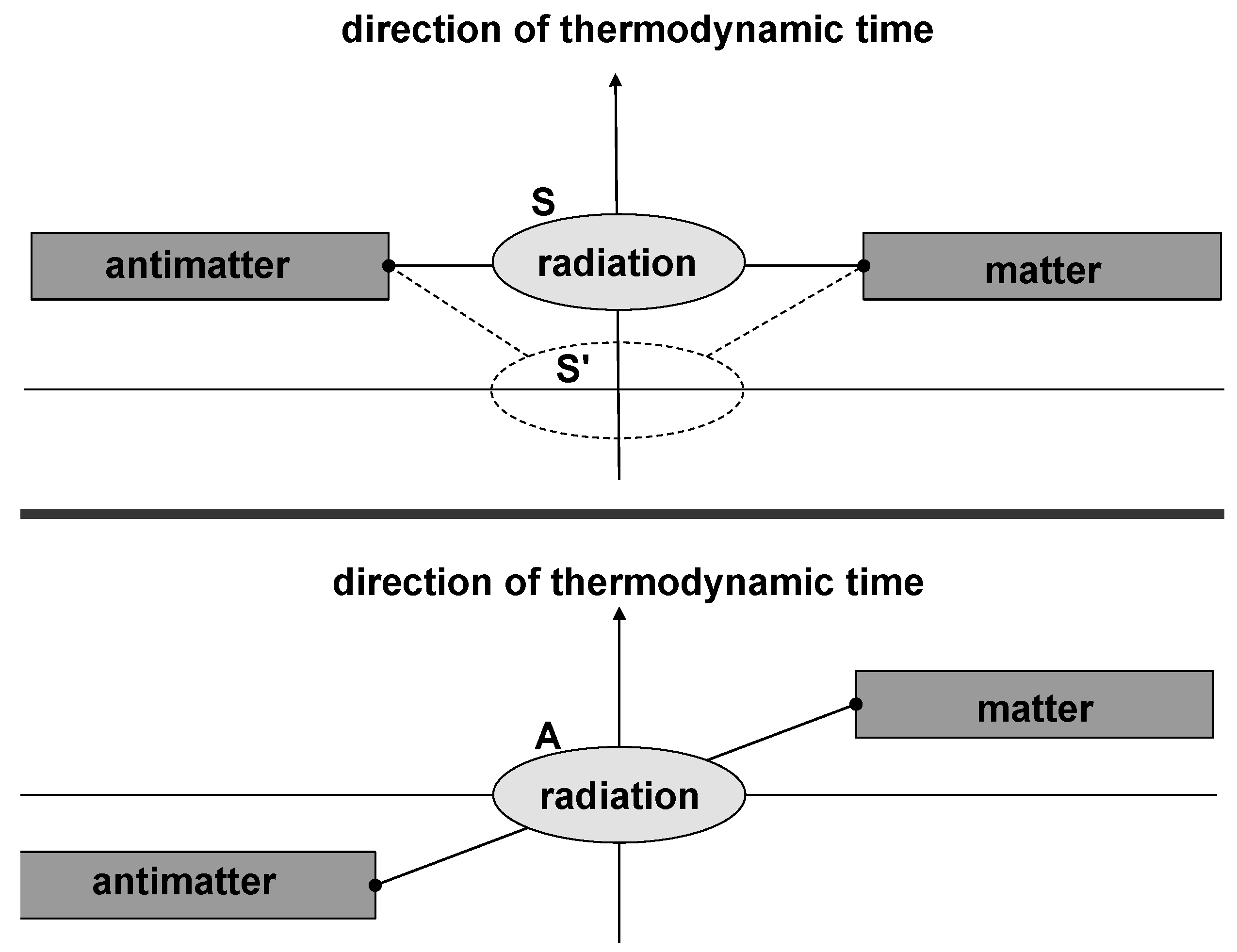
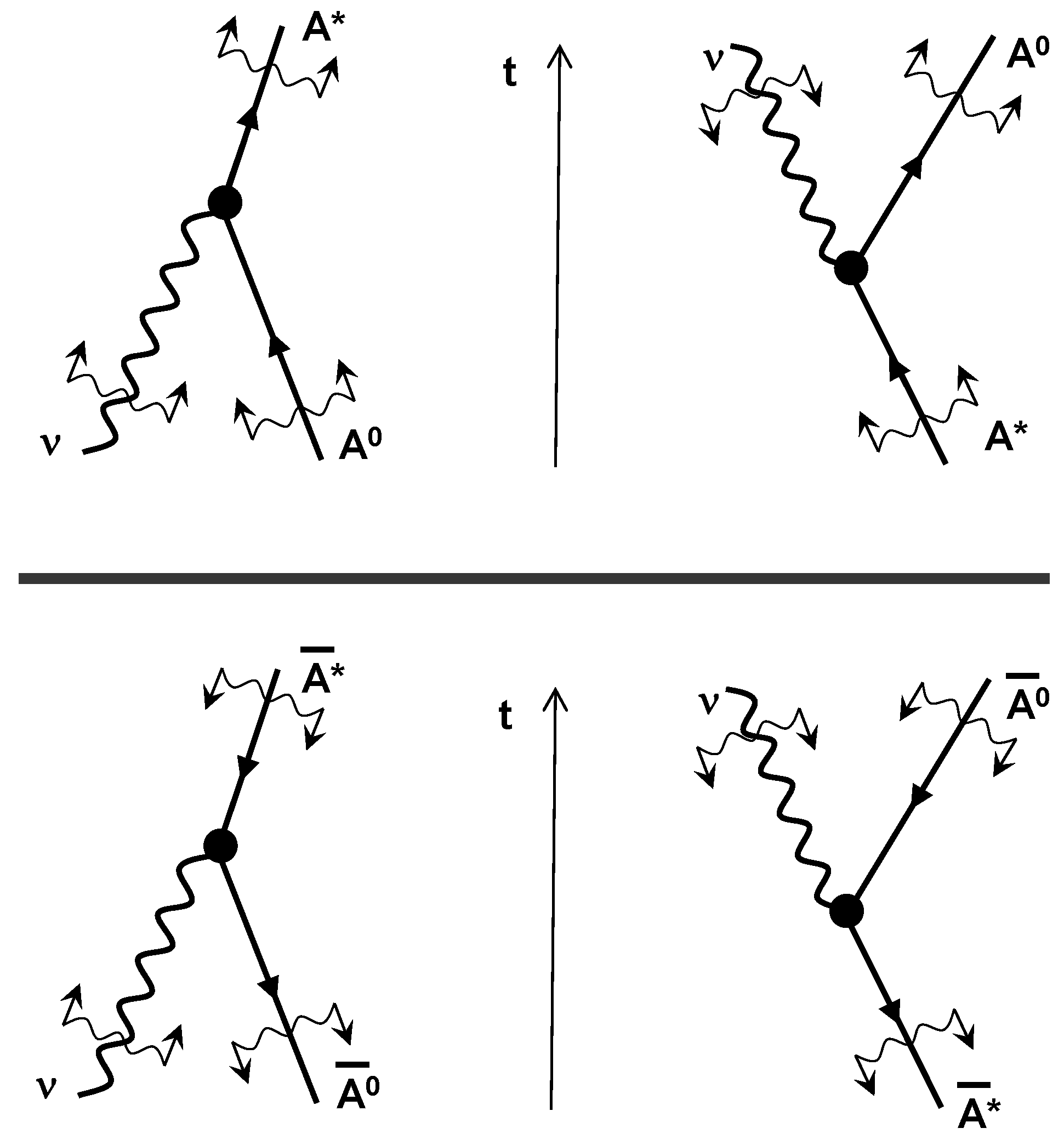
5. Interactions of Radiation and Antimatter

This section considers the interaction of radiation and matter assuming that (1) radiation is decoherence-neutral and (2) antimatter is dominated by recoherence, in accordance with antisymmetric thermodynamics. The utility of these assumptions is self-evident: under symmetric assumptions, interactions of radiation and antimatter would simply be identical to the corresponding interactions of radiation and matter.

The photon/antimatter interaction, which is shown in Figure 4 (bottom) is similar to the photon/matter interaction but antimatter recoheres instead of decohering. Interactions of a single quantum state populated by q photons with $F_{\mathsf{Ā}}$ antimatter atoms is specified by the reactions

$$\left(1\right){\mathsf{Ā}}^{\circ }+\nu ⟶{\mathsf{Ā}}^{*}\mathrm{and}\left(2\right){\mathsf{Ā}}^{*}⟶{\mathsf{Ā}}^{\circ }+\nu$$

(37)

The number of reactions per reaction time $\tau$ is given by

$$\Delta q_1=K{f}_{{\mathsf{Ā}}^{*}}^{″}{q}^{\prime }H\left(f_{{\mathsf{Ā}}^{\circ }}^{\prime }\right)$$

(38)

for the absorption reaction, where $f_{{\mathsf{Ā}}^{*}}^{″}\approx f_{{\mathsf{Ā}}^{*}}^{\prime }$ and $q^{\prime }=q^{″}+1\ne q^{″}$ and

$$\Delta q_2=K{f}_{{\mathsf{Ā}}^{\circ }}^{″}{q}^{″}H\left(f_{{\mathsf{Ā}}^{*}}^{\prime }\right)$$

(39)

for the emission reaction, where $f_{{\mathsf{Ā}}^{\circ }}^{″}\approx f_{{\mathsf{Ā}}^{\circ }}^{\prime }$ and $q^{″}=q^{\prime }+1\ne q^{\prime }$. With $q^{\prime }=q$ and $\Delta q=\Delta q_2-\Delta q_1$, the forward-time kinetics rate equation takes the form

$$\begin{array}{cc}\hfill \frac{dq}{dt}& =k(q+1)f_{{\mathsf{Ā}}^{\circ }}H\left(f_{{\mathsf{Ā}}^{*}}\right)-kq{f}_{{\mathsf{Ā}}^{*}}H\left(f_{{\mathsf{Ā}}^{\circ }}\right)\hfill \\ & \underset{f_{{\mathsf{Ā}}^{\circ }},f_{{\mathsf{Ā}}^{*}}>0}{=}k\left(f_{{\mathsf{Ā}}^{\circ }}-q\left(f_{{\mathsf{Ā}}^{*}}-f_{{\mathsf{Ā}}^{\circ }}\right)\right)\hfill \end{array}$$

(40)

The Heaviside constraints cannot generally be omitted in this case.

A stable equilibrium solution of (40) is possible only when $f_{{\mathsf{Ā}}^{*}}>f_{{\mathsf{Ā}}^{\circ }}$ and $T=-\overline{T}>0$ in the Gibbs distribution of antimatter

$$\frac{f_{{\mathsf{Ā}}^{*}}}{f_{{\mathsf{Ā}}^{\circ }}}=\exp \left(-\frac{\Delta E}{\overline{T}}\right)$$

(41)

The solution is consistent and is specified by Bose-Einstein distribution (33). If, however, $T=-\overline{T}<0$ and $f_{{\mathsf{Ā}}^{*}}<f_{{\mathsf{Ā}}^{\circ }},$ then Equation (40) is unstable and q would grow exponentially similar to the exponential growth mentioned in the previous section, although unlike in the previous section the process never reaches a thermal equilibrium. As q increases, $f_{{\mathsf{Ā}}^{*}}$ decreases and $f_{{\mathsf{Ā}}^{\circ }}$ increases due to conservation of energy and this further stimulates emission specified by Equation (40). Emission is terminated only when the excited population of atoms is exhausted $f_{{\mathsf{Ā}}^{*}}=0$. At this stage, the antimatter falls into the ground state. This behaviour is expected since the apparent temperature of antimatter T is a negative of its intrinsic temperature $\overline{T}$ and, as noted in the previous section, the equilibrium with radiation can be achieved only at positive apparent temperatures T.

The most interesting feature is that the step by step equations considered here are exactly CPT-invariant: i.e., (30) and (31) can be converted into (38) and (39) by swapping A with Ā and t with $-t$ (changing the direction of time implies swapping “prime” with “double prime” and the forward reaction rate $\Delta q_1$ with the reverse reaction rate $\Delta q_2$). Equations (32) and (40), however, do not represent the exact time inverse of each other and this is not a mistake. Reaction rate Equations (32) and (40) are formulated for conditions of dominant forward causality, when we set initial conditions and not the final conditions. Both of these equations are to be solved forward in time t. Equation (40) would become the exact time inverse of (32), if the antimatter equation was formulated for a problem with final conditions. The environment, which has predominant forward direction of thermodynamic time, interferes with our localised consideration forcing us to set initial and not final conditions in our gedanken experiments. As discussed in Reference [37], this kind of interference is CP-invariant (and not CPT-invariant), which can lead to apparent CPT violations: inconsistency between (32) and (40) in the present case. This violation is not a genuine violation of CPT symmetry—it would disappear if matter was changed to antimatter not only in our experiment but also everywhere in the Universe [37]. The environmental interference with the initial/final conditions, however, does not affect the exact CPT symmetry of Equation (10) derived for weak interactions of matter and antimatter. Being decoherence-neutral, radiation is affected more than matter and antimatter by the prevailing direction of decoherence in the environment.

The main outcomes of this section are summarised in form of the following proposition:

Proposition 5.

The antisymmetric (CPT-invariant) approach to thermodynamics and kinetics allows for stable equilibrium in interactions of radiation and antimatter but only if the intrinsic temperature of antimatter is negative. Positive intrinsic temperatures of antimatter result in radiation instabilities bringing the antimatter into its intrinsic ground state.

Assuming that the overall energy is preserved, $F_{{\mathsf{Ā}}^{*}}+q=\mathrm{const}$ and that $F_{{\mathsf{Ā}}^{*}},d{F}_{{\mathsf{Ā}}^{\circ }}>0$, we can write

$$-\frac{d{F}_{{\mathsf{Ā}}^{*}}}{dt}=\frac{d{F}_{{\mathsf{Ā}}^{\circ }}}{dt}=\frac{dq}{dt}=k\left((q+1)f_{{\mathsf{Ā}}^{\circ }}-q{f}_{{\mathsf{Ā}}^{*}}\right)$$

(42)

considering intrinsic entropies $S_{\nu }$ and $S_{\mathsf{Ā}}$ defined by (34) and (20), the H-theorem can be formulated as

Proposition 6.

For interactions of radiation and antimatter, the symmetric $S_s=S_{\nu }+S_{\mathsf{Ā}}$ and antisymmetric $S_a=S_{\nu }-S_{\mathsf{Ā}}$ entropies are increased forward in time t by, correspondingly, symmetric and antisymmetric kinetics until the evolution reaches its equilibrium or is terminated by physical constraints.

Since the case of symmetric kinetics is equivalent to interactions of radiation and matter and, thus, is obvious, we prove the H-theorem only for the antisymmetric case:

$$\begin{array}{cc}\hfill \frac{d{S}_a}{dt}& =\frac{dq}{dt}\ln \left(\frac{1+q}{q}\right)+\sum _{{\mathrm{X}=\mathsf{Ā}}^{*},{\mathsf{Ā}}^{\circ }}\frac{d{F}_{{}_{\mathrm{X}}}}{dt}\left(\ln \left(f_{\mathrm{X}}\right)+1\right)=\hfill \\ & =k\left((q+1)f_{{\mathsf{Ā}}^{\circ }}-q{f}_{{\mathsf{Ā}}^{*}}\right)\ln \left(\frac{\left(1+q\right)f_{{\mathsf{Ā}}^{\circ }}}{q{f}_{{\mathsf{Ā}}^{*}}}\right)\ge 0\hfill \end{array}$$

(43)

for any positive $q,$ $f_{{\mathsf{Ā}}^{*}}$ and $f_{{\mathsf{Ā}}^{\circ }}$. The evolution is terminated $d{S}_a/dt=0$ if the physical boundary (i.e., $F_{{\mathsf{Ā}}^{*}}=0$ or $F_{{\mathsf{Ā}}^{\circ }}=0$) is reached.

6. Discussion and Conclusions

One of the main conclusions of the present work in the context of interactions of radiation and matter is neutrality of radiation with respect to decoherence and recoherence: neither of these processes can dominate the other. Radiation tends to decohere before and recohere after its interactions with matter and antimatter. Only decoherence-neutral treatment of radiation matches the Einstein theory [27] and experimental evidence [38]. While our world is dominated by decoherence, presence of recoherence in interactions of radiation with matter was envisaged a hundred years ago by the insights of the Einstein radiation theory and later experimentally confirmed by existence of lasers. Unlike low-temperature Bose condensates, which are forced into a single quantum state by the energy constraint, the most spectacular display of dynamic recoherence in lasers occurs at high temperatures with plenty of quantum states to select from. Does the conclusion of decohering neutrality of radiation have any implications for choosing between symmetric and antisymmetric extensions of thermodynamics into antimatter?

According to the antisymmetric view of thermodynamic interactions of matter and antimatter, decoherence occurs in opposite temporal directions for matter and antimatter. Since radiation is neutral with respect to the matter/antimatter duality, there could not be a direction of decoherence intrinsically associated with radiation (Figure 5, bottom). Yet, radiation must decohere during interactions with matter (antimatter); at least to some extent since, otherwise, concepts of statistical physics would not be applicable to these interactions, which is obviously incorrect. In the antisymmetric treatment of the problem, radiation does not have any intrinsic decohering mechanisms on its own, but interactions of radiation with matter (antimatter) should cause radiation decoherence and recoherence.

While decohering neutrality of radiation and physical existence of recoherence make this antisymmetric approach to thermodynamics and kinetics rather attractive, it does not prove the approach. Matter and antimatter can still have the same direction of the thermodynamic time, while radiation having no temporal preference as shown by in Figure 5 (top, case S${}^{\prime }$). The neutrality of radiation only forces us to discard theories presuming that decoherence is caused by interactions with universal fields (such as gravity—see Reference [3]) since photons should not interact with these fields. However, other fields (e.g., the Higgs field) may have the desired decohering effect on particles and antiparticles, but no effect on photons.

While the symmetric and environmental mechanisms of decoherence are more conceptually aligned with presence of a time priming field, and the antisymmetric decoherence generally points in the direction of intrinsic mechanisms as possible sources of the time asymmetry, this work concludes that both mechanisms are likely to be important. The major challenge in experimental testing of the invariant properties of thermodynamics is in creating an antisystem—a thermodynamic system made of antimatter. Since the mechanism of thermodynamic time remains unknown, it is not clear how large this antisystem needs to be. One of the smallest possible antisystems might be represented by quark-gluon plasma produced in collision of antibaryons, although the extent of thermodynamic properties that can exists at these very small scales is not fully known [21].

It seems that the best approach for testing the invariant properties of thermodynamics is in trapping a statistical set of antiatoms, investigating their emission/absorption properties and comparing them with the conventional thermodynamic properties for emission/absorption by a similar set of atoms. The analysis of Section 4 and Section 5 indicates that, in symmetric thermodynamics, both sets should have exactly the same properties. However, the antiatoms are expected to fall into their intrinsic ground states according to antisymmetric thermodynamics. This does not mean that a particular antiatom cannot be in an excited state but only that this state is thermodynamically unlikely in statistical antisystems. The absorption/emission properties of any isolated quantum objects and antiobjects that do not display thermodynamic properties are expected to be CP-invariant; it is only thermodynamic antisystems that behave unconventionally in antisymmetric thermodynamics. Since the antiatoms are likely to be gathered in very small quantities, reaching the statistical scales becomes a major issue. Antisymmetric thermodynamics predicts that an antiatom system would be more reluctant to absorb light than the corresponding atom system, and this asymmetry should be more evident for larger systems (i.e., for systems that are sufficiently large to exhibit thermodynamic properties). In antisymmetric thermodynamics, equilibrium between radiation and antimatter is theoretically possible but (under normal conditions) not practically, since this equilibrium requires negative intrinsic temperatures of antimatter. Rapid progress in antimatter creation and spectroscopy suggests that it might be possible to conduct these experiments with existing levels of technology [39,40].

References

1. Boltzmann, L. Lecures on Gas Thoery; University of California Press: Berkeley, CA, USA, 1964. [Google Scholar]
2. Price, H. Time’s Arrow and Archimedes’ Point: New Directions for the Physics of Time; Oxford University Press: Oxford, UK, 1996. [Google Scholar]
3. Penrose, R. Road to Reality: A Complete Guide to the Laws of the Universe; A. Knopf: New York, NY, USA, 2005. [Google Scholar]
4. Zeh, H.D. The Physical Basis of The Direction of Time, 5th ed.; Springer: New York, NY, USA, 2007. [Google Scholar]
5. Abe, S. Maximum-power quantum-mechanical Carnot engine. Phys. Rev. E 2011, 83, 041117. [Google Scholar] [CrossRef] [PubMed]
6. Gogolin, C.; Eisert, J. Equilibration, thermalisation, and the emergence of statistical mechanics in closed quantum systems. Rep. Prog. Phys. 2016, 79, 056001. [Google Scholar] [CrossRef] [PubMed]
7. Klimenko, A.; Maas, U. One Antimatter-Two Possible Thermodynamics. Entropy 2014, 16, 1191–1210. [Google Scholar] [CrossRef]
8. Klimenko, A.Y. Symmetric and antisymmetric forms of the Pauli master equation. Sci. Rep. 2016, 6, 29942. [Google Scholar] [CrossRef] [PubMed]
9. Sakharov, A.D. Violation of CP invariance, C asymmetry, and baryon asymmetry of the universe. J. Exp. Theory Phys. 1967, 5, 24–27. [Google Scholar]
10. Pauli, W. Uber das H-Theorem vom Anwachsen der Entropie vom Standpunkt der neuen Quantenmechanik. In Probleme der Modernen Physik. Arnold Sommerfeld zum 60 Geburtstage; Hirzel: Leipzig, Germany, 1928; pp. 30–45. (In German) [Google Scholar]
11. Zurek, W.H. Decoherence and the Transition from Quantum to Classical—Revisited. Los Alamos Sci. 2002, 27, 86–109. [Google Scholar]
12. Bassia, A.; Ghirardi, G. Dynamical reduction models. Phys. Rep. 2003, 379, 257–426. [Google Scholar] [CrossRef]
13. Beretta, G. On the general equation of motion of quantum thermodynamics and the distinction between quantal and nonquantal uncertainties (MIT, 1981). arXiv, 2005; arXiv:quant-ph/0509116. [Google Scholar]
14. Stamp, P.C.E. Environmental decoherence versus intrinsic decoherence. Philos. Trans. Ser. A Math. Phys. Eng. Sci. 2012, 370, 4429. [Google Scholar] [CrossRef] [PubMed]
15. Zurek, W.H. Environment-induced superselection rules. Phys. Rev. Lett. 1982, 26, 1862–1888. [Google Scholar] [CrossRef]
16. Joos, E.; Kiefer, C.; Zeh, H.D. Decoherence and the Appearance of a Classical World in Quantum Theory, 2nd ed.; Springer: Berlin/Heidelberg, Germany, 2003. [Google Scholar]
17. Schlosshauer, M. Decoherence, the measurement problem, and interpretations of quantum mechanics. Rev. Mod. Phys. 2005, 76, 1267–1305. [Google Scholar] [CrossRef]
18. Goldstein, S.; Lebowitz, J.L.; Tumulka, R.; Zanghi, N. Canonical typicality. Phys. Rev. Lett. 2006, 96, 050403. [Google Scholar] [CrossRef] [PubMed]
19. Popescu, S.; Short, A.J.; Winter, A. Entanglement and the foundations of statistical mechanics. Nat. Phys. 2006, 2, 754–758. [Google Scholar] [CrossRef]
20. Yukalov, V. Equilibration and thermalization in finite quantum systems. arXiv, 2012; arXiv:1201.2781. [Google Scholar]
21. Braun-Munzinger, P.; Stachel, J. The quest for the quark-gluon plasma. Nature 2007, 448, 302–309. [Google Scholar] [CrossRef] [PubMed]
22. Aharonov, Y.; Bergmann, P.; Lebowitz, J. Time Symmetry in the Quantum Process of Measurement. Phys. Rev. B 1964, 134, 1410. [Google Scholar] [CrossRef]
23. Wharton, K.B. Time-Symmetric Quantum Mechanics. Found. Phys. 2007, 37, 159–168. [Google Scholar] [CrossRef]
24. Aharonov, Y.; Vaidman, L. The Two-State Vector Formalism: An Updated Review. Lect. Notes Phys. 2008, 734, 399–447. [Google Scholar]
25. Dyson, F.J. The radiation theories of Tomonaga, Schwinger, and Feynman. Phys. Rev. 1949, 75, 486–502. [Google Scholar] [CrossRef]
26. Landau, L.D.; Lifshits, E.M. Course of Theoretical Physics Vol. 3: Qunatum Mechanics; Butterworth-Heinemann: Oxford, UK, 1980. [Google Scholar]
27. Einstein, A. The Quantum Theory of Radiation. Phys. Z. 1917, 18, 121. [Google Scholar]
28. Dirac, P.A.M. The Quantum Theory of the Emission and Absorption of Radiation. Proc. R. Soc. Lond. A Math. Phys. Eng. Sci. 1927, 114, 243–265. [Google Scholar] [CrossRef]
29. Fermi, E. Quantum Theory of Radiation. Rev. Mod. Phys. 1932, 4, 87–132. [Google Scholar] [CrossRef]
30. Berestetskii, V.; Lifshitz, E.; Pitaevskii, L. Course of Theoretical Physics Vol. 4: Quantum Electrodynamics; Butterworth-Heinemann: Oxford, UK, 1982. [Google Scholar]
31. Andrews, D. A unified theory of radiative and radiationless molecular energy transfer. Chem. Phys. 1989, 135, 195–201. [Google Scholar] [CrossRef]
32. Griffiths, D. Introduction to Quantum Mechanics, 2nd ed.; Prentice Hall: Upper Saddle River, NJ, USA, 2005. [Google Scholar]
33. Salam, A. Molecular Quantum Electrodynamics: Long-Range Intermolecular Interactions; John Wiley and Sons: Hoboken, NJ, USA, 2010. [Google Scholar]
34. Ramsey, N.F. Thermodynamics and Statistical Mechanics at Negative Absolute Temperatures. Phys. Rev. 1956, 103, 20–28. [Google Scholar] [CrossRef]
35. Landau, L.D.; Lifshits, E.M. Course of Theoretical Physics Vol. 5: Statistical Physics; Butterworth-Heinemann: Oxford, UK, 1980. [Google Scholar]
36. Klimenko, A.Y. Teaching the third law of thermodynamics. arXiv, 2012; arXiv:1208.4189. [Google Scholar]
37. Klimenko, A. Note on invariant properties of a quantum system placed into thermodynamic environment. Phys. A Stat. Mech. Appl. 2014, 398, 65–75. [Google Scholar] [CrossRef]
38. Haken, H. Light (v1: Waves, Photons, Atoms, v2: Laser Light Dynamics); North-Holland Pub.: Amsterdam, The Netherlands, 1981. [Google Scholar]
39. Madsen, N. Cold antihydrogen: A new frontier in fundamental physics. Philos. Trans. R. Soc. A 2010, 368, 3671–3682. [Google Scholar] [CrossRef] [PubMed]
40. Andronic, A.; Braun-Munzinger, P.; Stachele, J.; Stöckera, H. Production of light nuclei, hypernuclei and their antiparticles in relativistic nuclear collisions. Phys. Lett. B 2011, 697, 203–207. [Google Scholar] [CrossRef]
41. Lloyd, S. Black Holes, Demons and Loss of Coherence. Ph.D. Thesis, The Rockefeller University, New York, NY, USA, 1988. [Google Scholar]
42. Bocchieri, P.; Loinger, A. Quantum Recurrence Theorem. Phys. Rev. 1957, 107, 337–338. [Google Scholar] [CrossRef]
43. Linden, N.; Popescu, S.; Short, A.J.; Winter, A. Quantum mechanical evolution towards thermal equilibrium. Phys. Rev. E 2009, 79, 061103. [Google Scholar] [CrossRef] [PubMed]
44. Beringer, J.; Arguin, J.F.; Barnett, R.M.; Copic, K.; Dahl, O.; Groom, D.E.; Lin, C.J.; Lys, J.; Murayama, H.; Wohl, C.G.; et al. The Review of Particle Physics. Phys. Rev. 2012, 86. [Google Scholar] [CrossRef]
45. Lees, J.P.; Poireau, V.; Tisserand, V.; Grauges, E.; Palano, A.; Eigen, G.; Brown, D.N.; Kolomensky, Y.G.; Koch, H.; Schroeder, T.; et al. Tests of CPT symmetry in B0 B ¯ 0 mixing and in B0c c ¯ K0 decays (BABAR Collaboration). Phys. Rev. D 2016, 94, 011101. [Google Scholar] [CrossRef]
Figure 1. Sequence of decoherence and unitary events in a reacting system.
Entropy 19 00202 g001
Figure 2. Energy exchange between particle and antiparticle in a thermodynamic system with the same direction of decoherence: forward (left) and reverse (right) reactions. Top: symmetric (CP-invariant) decoherence; bottom: antisymmetric (CPT-invariant) decoherence. The braced arrows show the direction of decoherence before and after the interaction.
Entropy 19 00202 g002
Figure 3. Interactions of radiation with matter: absorption (left) and emission (right). Top: radiation with predominant decoherence; bottom: radiation with predominant recoherence.
Entropy 19 00202 g003
Figure 4. Interactions of decoherence-neutral radiation with matter (top) and antimatter (bottom); absorption (left) and emission (right).
Entropy 19 00202 g004
Figure 5. Directions of thermodynamic time for matter, antimatter and radiation. (Top): symmetric (CP-invariant) approach; (bottom): antisymmetric (CPT-invariant) approach.
Entropy 19 00202 g005