Article

Low Complexity List Decoding for Polar Codes with Multiple CRC Codes

1
College of Information and Communication Engineering, Sungkyunkwan University, Gyeonggi-do, Suwon 16419, Korea
2
Department of Computer Science, Ulsan College, Hwajeong-dong, Dong-gu, Ulsan 44022, Korea
3
Department of Information and Communication Engineering, Chosun University, Gwangju 61452, Korea
*
Author to whom correspondence should be addressed.
Entropy 2017, 19(4), 183; https://doi.org/10.3390/e19040183
Submission received: 7 February 2017 / Revised: 22 March 2017 / Accepted: 11 April 2017 / Published: 24 April 2017
(This article belongs to the Section Information Theory, Probability and Statistics)

Abstract

:
Polar codes are the first family of error correcting codes that provably achieve the capacity of symmetric binary-input discrete memoryless channels with low complexity. Since the development of polar codes, there have been many studies to improve their finite-length performance. As a result, polar codes are now adopted as a channel code for the control channel of 5G new radio of the 3rd generation partnership project. However, the decoder implementation is one of the big practical problems and low complexity decoding has been studied. This paper addresses a low complexity successive cancellation list decoding for polar codes utilizing multiple cyclic redundancy check (CRC) codes. While some research uses multiple CRC codes to reduce memory and time complexity, we consider the operational complexity of decoding, and reduce it by optimizing CRC positions in combination with a modified decoding operation. Resultingly, the proposed scheme obtains not only complexity reduction from early stopping of decoding, but also additional reduction from the reduced number of decoding paths.

1. Introduction

Polar codes are the first family of error correcting codes that provably achieve the capacity for symmetric binary-input discrete memoryless channels (B-DMCs) with low complexity successive cancellation (SC) decoding [1]. Arikan introduced the channel polarization that splits the capacities of information channels to one or zero as block length becomes longer [1]. As a dual phenomenon of the channel polarization, the conditional entropies in source coding context are also polarized when the joint entropy is broken down by the chain rule (this phenomenon is called the “source polarization”) [2]. The source coding using polar codes based on the source polarization is also proven to be optimal for both lossless [3] and lossy source coding [4]. In addition, polar codes have been extended to multi-terminal problems such as multiple access and broadcast channels in channel coding [5,6,7,8], and Slepian–Wolf and Gelfand–Pinsker problems in source coding [9,10,11].
From the channel coding perspective, even though the SC decoding of polar codes achieves the capacity, it was not as competitive in finite length performance as low-density parity-check (LDPC) codes and turbo codes [12,13]. However, when both the concatenation of polar codes with cyclic redundancy check (CRC) codes and the SC list (SCL) decoding that keeps the best multiple decoding paths are used, the finite-length polar coding performance becomes comparable to the LDPC coding [12]. Furthermore, a parity-check concatenation was proposed to improve the performance of polar codes based on CRC-aided SCL decoding [14]. Recently, thanks to their excellent error performance and fine rate flexibility [15], polar codes have been adopted as a channel code for the control channel of 5G new radio of the 3rd generation partnership project [16].
In order for polar codes to show comparable error performance to the LDPC codes in moderate block lengths, the SCL decoding requires a rather large list size, e.g., L = 32 . The list size L determines the maximum number of decoding paths and affects the complexity of log-likelihood ratio (LLR) calculation and sorting of path metrics (PMs). It is a linear factor in the decoding complexity. According to [17,18], even for a list size smaller than 10, the SCL decoder has larger complexity than the LDPC decoder, which leads to a considerable gap in power consumption between those decoders. Therefore, a low complexity realization of the SCL decoding is important from a practical perspective, and some recent research has reduced the decoding complexity by efficiently managing decoding paths. In [19], decoding paths do not split when one of two child-paths is dominant. In addition, the decoding paths that have low reliability are eliminated during decoding in [20]. The operational decoding complexity of those schemes was lowered by the reduced average number of decoding paths.
Lately, some studies have used multiple CRC codes to address different complexity issues of the decoding [21,22,23]. The scheme in [21] aims to reduce the memory complexity by selecting only the most likely path after each CRC operation where more than one CRC is applied. In [22], the complexity reduction due to CRC-based early stopping of decoding was reported. Finally, the method in [23] reduces the worst decoding latency and space complexity for storing intermediate LLRs.
This paper addresses polar coding with multiple CRC codes similarly to [21,22,23], but we focus more on optimization of the scheme in terms of decoding complexity. First, we define the operational complexity, and then minimize it by optimizing CRC positions. In addition, the optimization of CRC positions is extended to a modified decoding that uses a complexity reduction trick called “instant decision” (first proposed in [24]). It is shown that the optimized CRC placement considerably lowers the decoding complexity of the multi-CRC scheme in a wide range of signal-to-noise ratio (SNR).
The rest of this paper is organized as follows. In Section 2, the SCL decoding and its operational complexity are introduced, and in Section 3, the encoding and decoding methods for the multi-CRC scheme, and the optimization algorithm for CRC positions are explained. Section 4 provides the performance and complexity of the proposed and conventional schemes, and Section 5 concludes this paper.

2. SCL Decoding and Its Operational Complexity

This section introduces the basics of polar coding and the conventional SCL decoding [12,13], and also defines the operational complexity of the SCL decoding with regard to hardware implementation.

2.1. Polar Encoding and SCL Decoding

We only consider binary polar codes with the kernel matrix F = 1 0 1 1 and n-fold polarization, where n is a positive integer. Then, for N = 2 n copies of a given symmetric B-DMC W, the channel combining and splitting generate N split channels whose capacities polarize to one or zero [1]. The fraction of good split channels approaches the capacity of W as N goes to infinity. This phenomenon is called the “channel polarization”. Polar coding transmits information through the good split channels that have higher capacity. The index set of the good split channels is called the “information set”, and is denoted by A . For a row vector u = ( u 1 , u 2 , . . . , u N ) consisting of the information part ( u i : i A ) and the frozen part ( u i : i A c ) , the codeword vector is given as x = ( x 1 , x 2 , . . . , x N ) = uG N where G N = B N F n is the generator matrix, and B N is the bit-reversal permutation matrix (see [1] for more details). If | A | = K , the code rate R is equal to K / N .
SC decoding is the first decoding method of polar codes [1]. Each element of u is successively decoded in the increasing order of index. At the i-th decoding step, if i A c , u ^ i is set as a frozen bit. Otherwise, u i  is decided by a maximum likelihood (ML) rule such as u ^ i = argmax u i = 0 , 1 Pr ( y , ( u ^ 1 , . . . , u ^ i 1 ) | u i ) with the aid of the previously estimated vector ( u ^ 1 , . . . , u ^ i 1 ) , where y is the output of the vector channel of W. When  i = 1 , ( u ^ 1 , . . . , u ^ i 1 ) is defined as a void. At last, the SC decoder outputs u ^ , which corresponds to a single decoding path.
Later, SCL decoding was proposed to improve the error performance of finite-length polar codes [13]. The SCL decoding maintains a list of L most likely paths down to the bottom of the decoding tree as depicted in Figure 1. At the decoding step of an information u i , the number of decoding paths is doubled until the list size reaches L without path selection. If the number of candidate paths reached L, then, in the next step, 2 L paths are generated and the best L paths are selected based on their PMs. For a frozen bit, the number of paths does not need to increase because we have only to take a valid child branch for each path. Finally, after decoding of all u i ’s, the best path is selected among L survivors.
The CRC concatenation before polar encoding and CRC-aided SCL decoding are used to further improve the error performance [12]. In [12], the message is CRC-encoded and its parity is usually appended at the end of the message. The CRC code is used for the verification of survived decoding paths at the last stage of SCL decoding. If the CRC code of length P is concatenated, then | A | = K + P , but the code rate R is maintained as K / N . In this paper, the polar code that uses a single CRC code is termed the “Single CRC (SCRC) scheme”.

2.2. Operational Complexity of the SCL Decoding for the SCRC Scheme

Because our concern is related to the overall computational complexity, we first define the operational complexity of a hardware-friendly LLR-based SCL decoding algorithm for the SCRC scheme. The overall complexity is counted in the number of addition-equivalent operations or simply additions for convenience.
There are three main operations that largely affect the complexity. The first operation is the LLR calculation for the information vector u in terms of the split channels. The SCL decoding runs the SC algorithm for each of all L decoding paths. Therefore, two types of LLR calculations are used as in the SC decoding. Note that the exact expressions for LLR calculation exist [25], but we consider their approximations preferred in implementation:
γ c = sgn ( α ) sgn ( β ) min ( | α | , | β | ) ,
γ v = β + ( 1 ) u α ,
where α and β are the input LLRs, and u is the input bit, and sgn ( · ) returns the sign of the argument [25,26,27]. Figure 2 shows the associated graph, where squares and circles represent the check and variable nodes, respectively. Those operations are termed the “check/variable node operation”, respectively. Each node operation can be implemented with a single addition or its equivalent [25]. Consequently, the total computational complexity can be counted in the number of additions.
Note that an SC decoding requires N log 2 N additions [1]. For the SCL decoding, roughly the list size L is a linear factor in complexity. However, the list size and the number of candidate decoding paths do not need to be the maximal size L during an entire decoding. The temporary list size can be taken into account. The change in complexity calculation regarding the temporary list size is not negligible. Let us denote the temporary number of decoding paths of the i-th decoding step by l i . More precisely, l i is the number of existing paths before the decoding or processing of u i . The temporary list size does not increase if u i is a frozen bit or l i = L .
The transience of the list size in a decoding progress is shown in Figure 1. The temporary list size may increase slowly in the beginning because the front of sequence u is mostly filled with frozen bits. When the sum of the numbers of check and variable node operations at the i-th SC decoding is denoted by n i , the total number of node operations for an entire SCL decoding is i = 1 N l i n i . Algorithm 1 calculates l i , and we denote this function by f ( · ) . The function f ( A , l i , i ) returns l i + 1 for 1 i N 1 (set l 1 = 1 ). Here, l i + 1 is computed based on the SCL algorithm by checking whether i A or not. Furthermore, n i is j = 0 t 2 j where t is the number of consecutive zeros of ( i 1 ) 2 from the rightmost bit [1]. For example, when N = 8 and i = 7 , ( i 1 ) 2 = 110 and t is 1.
Algorithm 1 Calculation of l i + 1 for the SCL decoding, f( A , l i , i)
Require: A , l i , i
Ensure: l i + 1
1:
 if i A then
2:
  if 2 l i L then
3:
    l i + 1 2 l i ;  
4:
  else
5:
    l i + 1 L
6:
  end if 
7:
 else
8:
   l i + 1 l i
9:
 end if 
10:
 return l i + 1 ;
Second, sorting of PMs is considered for complexity evaluation. When an information bit is decoded, the sorting of 2 l i 2 L PMs is needed at the i-th decoding step. In this paper, the complexity of sorting is represented in the number of additions. The sorting complexity depends on the type of sorting [25]. Although a parallel sorting is preferred for fast decoder realization, a serial sorting is also taken into account for minimal complexity reference. The quick sorter that requires 2 l i log 2 ( 2 l i ) comparisons for 2 l i paths is considered for a serial sorter. For a parallel sorter, we adopt the bitonic sorter [17] requiring ( l i / 2 ) log 2 ( 2 l i ) ( log 2 ( 2 l i ) + 1 ) comparisons because it gives a good complexity-speed tradeoff. If we assume the bitonic sorter, the number of comparisons at the i-th decoding step, s i , is computed as
s i = ( l i / 2 ) log 2 ( 2 l i ) ( log 2 ( 2 l i ) + 1 ) , if i A and 2 l i > L , 0 , otherwise .
We evaluate the sorting complexity in the number of additions since a comparison is equivalent to an addition.
Finally, the calculation of PM should be counted. PM calculation can also be approximated by a single addition as follows [25]:
PM i l = PM i 1 l , if u i l = ( 1 / 2 ) ( 1 sgn ( LLR i l ) ) , PM i 1 l + | LLR i l | , otherwise ,
where l ( 1 l 2 l i ) is the path index and LLR i l is the LLR for u i l [25].
The total decoding complexity C S for the SCRC scheme is the sum of the complexities of the node and sorting operations, and the PM calculation as
C S = ( l i + l i n i + s i ) = C S i ,
where C S i l i + l i n i + s i is the temporal complexity of the i-th decoding step of the SCRC scheme.
We omit CRC computation in complexity evaluation because it is composed of bit operations which are much lighter than real additions.

3. Low Complexity SCL Decoding with Multiple CRC Codes

As the list size L increases, the performance of the SCL decoding is improved, but the operational complexity also increases. Actually, in the LLR-based SCL decoding under consideration, the total operational complexity is the sum of C S i as in Equation (5), where each contributing term at C S i is linearly or slightly superlinearly related with l i . Therefore, the goal of this work is to reduce the operational complexity of the SCL decoding by managing the temporary list size lower by the aid of multiple CRC codes.
Previous research utilized multiple CRC codes to reduce the memory and time complexity of the corresponding SCL decoding [21,23]. Although multiple CRC codes were used to reduce the operational complexity in [22], in the complexity evaluation, the temporary list size was not counted and only uniform (equal-length) message partitioning was considered.
However, we consider the operational complexity reduction via nonuniform message partitioning and temporary list size management. If we can keep the temporary list size small, the overall complexity can be reduced. In this paper, in order to minimize the complexity effectively, the positions of CRC codes are optimized and a modified SCL decoding is employed.

3.1. Encoding and Decoding of the J-Tuple CRC Scheme

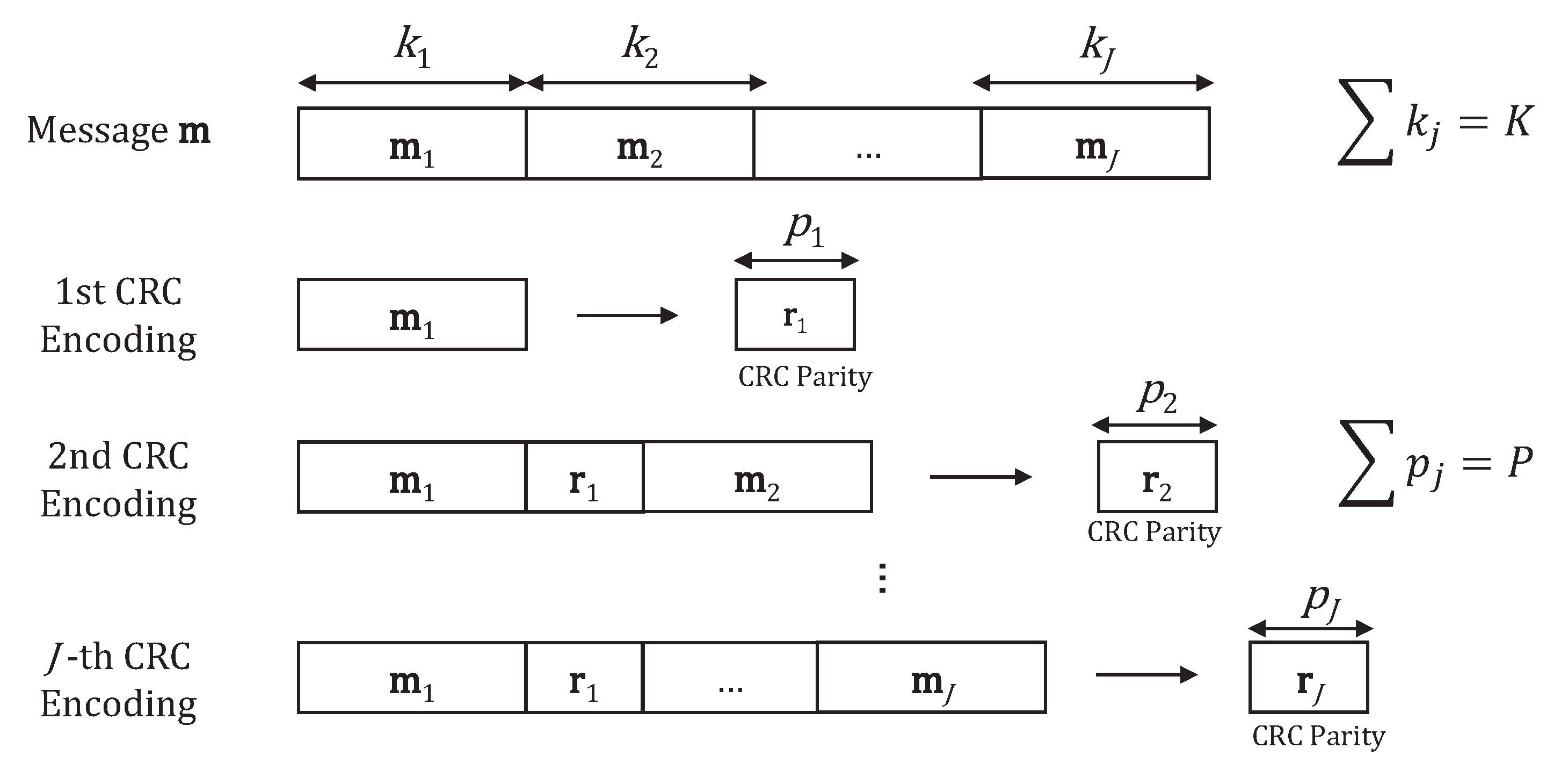
Let us consider a precoding of a partitioned message block with multiple CRC codes, followed by polar encoding. Before the polar encoding, the message vector m is partitioned into J subblocks ( m 1 , m 2 , . . . , m J ) , and they are encoded serially with J-tuple CRC codes as shown in Figure 3. A CRC encoding is carried out recursively to the concatenation of a CRC encoded block and a message subblock. CRC code lengths are defined by ( p 1 , p 2 , . . . , p J ) , and the CRC parities are denoted by ( r 1 , r 2 , . . . , r J ) . Through this nested encoding structure, undetected error by previous CRCs can be detected by following CRCs. The length of j-th message subblock is denoted by k j and the total sum of k j is K. Likewise, the total sum of p j is P. The CRC encoded message is encoded by a polar code. This scheme is termed the “J-tuple CRC scheme”. In this scheme, the lengths of J message subblocks can be determined by optimization of CRC positions that will be explained in Section 3.2.
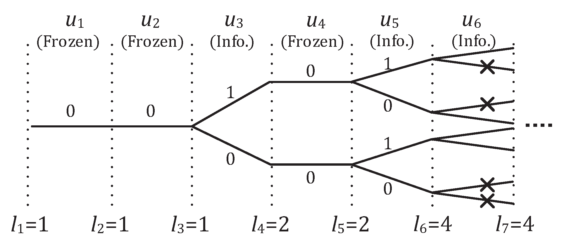
We introduce a decoding scheme for the J-tuple CRC scheme that is described in Algorithm 2. The temporary list size update is included in Algorithm 2 for a better presentation of the decoding procedure. The decoding is based on the conventional SCL decoding. However, the decoding is different in two aspects. First, J 1 CRC operations are additionally conducted to discard incorrect paths (lines 12–13 in Algorithm 2). Thus, due to the added J 1 CRCs, the temporary list size vector l = ( l 1 , l 2 , . . . , l N ) varies depending on the decoding instance. Note, however, l of the SCRC scheme is invariant because decoding path validity is checked only once at the bottom of the decoding tree. If any of the CRCs fail in all decoding paths during the decoding, then the decoding is terminated and a block error is declared. This event is called “early stopping” that is rare at a high SNR but frequent at a low SNR. If the decoder finds paths with valid CRC, all such paths proceed to the next step. Note that we do not assume that best effort decoding is required.
Algorithm 2 The ID-SCL decoding for the J-tuple CRC scheme
Require: Received vector, A , A g , k , p
Ensure: Estimated codeword
1:
  l 1 1 ;
2:
 for i = 1 : N do
3:
  if i A then
4:
   if i A g then
5:
    SCL decoding of u i maintaining number of survival paths and l i + 1 l i ;
6:
   else
7:
    SCL decoding of u i with list size of min ( 2 l i , L ) and l i + 1 min ( 2 l i , L ) ;
8:
   end if
9:
  else
10:
   Frozen bit decoding and l i + 1 l i ;
11:
  end if 
12:
  if i indicates the last parity bit of the j-th CRC then
13:
   Discard jth-CRC-invalid paths and update l i + 1 ;
14:
  end if
15:
 end for 
16:
 return ML codeword that passes the J-th CRC;
At each CRC operation, only valid paths—from a CRC perspective—survive so that the temporary list size is spontaneously reduced to one or just a few. The temporary list grows as the decoding proceeds, but if frozen bits follow consecutively, then the growth can progress slowly. This sporadic reduction of temporary list due to multiple CRC operations induces non-negligible complexity reduction.
Second, we consider a simple complexity reduction criterion for list management that was first proposed in [24] for reduction of sorting complexity. When a highly reliable bit is processed, the list is forced not to grow (lines 4–5 in Algorithm 2) and the sorting operation is skipped. Let A g be the set of indices where the capacity of corresponding split channels exceeds a certain threshold. ( A g  may alternatively be defined in terms of bit error rate.(period position)) When u i is processed, if i A g , we run the SC decoding instead of SCL decoding. The SC decoding decides the value of u i so that the temporary list size is maintained as l i + 1 = l i even if l i < L . Because u i for i A g is highly reliable, the correct path may not be ruled out by the value decision of u i . The list decoding with this criterion is termed the “instant-decision-aided SCL (ID-SCL) decoding”. (Here, we view the conventional SCL decoding operation as a delayed decision.)
In fact, the instant decision significantly reduces the complexity even though multiple CRC codes are not applied because it skips sorting operations that account for a large portion of the total complexity. In addition, the instant decision also has an effect of maintaining the temporary list size lower. Therefore, it is expected that the multi-CRC scheme including its optimization can also reduce the complexity under the ID-SCL decoding.
In the next subsection, the method of how to optimize CRC positions and determine A g is explained based on the aforementioned encoding and decoding methods. Note, however, that the J-tuple CRC scheme can be decoded with or without the instant bit decision. Obviously, CRC positions can be also optimized without the instant decision. The decoding without the instant decision is called the basic SCL decoding for the J-tuple CRC scheme.

3.2. Optimization of J-Tuple CRC Positions with Respect to Complexity

We can optimize the positions of CRCs to minimize the operational decoding complexity of the J-tuple CRC scheme. However, as mentioned above, since the decoding complexity of the J-tuple CRC scheme is variable depending on the decoding instance, we perform the optimization considering the average complexity based on the assumption that errors occur randomly in wrong paths. In order to simplify the problem, we input predetermined lengths of the J-tuple CRC codes ( p 1 , p 2 , . . . , p J ) into the optimization. Through decoding experiments, we determine ( p 1 , p 2 , . . . , p J ) empirically with regard to performance and complexity such that p j = P , where P is the CRC length of the compared SCRC scheme. In addition, because the minimum distance of the CRC concatenated polar code is affected by the length of the last CRC, we allocate more bits to the last CRC code than others.
Now let us first consider optimization of the positions of J CRCs under the basic SCL decoding. Note that the CRC positions are determined by the lengths of message subblocks. As mentioned, the basic SCL decoding for the J-tuple CRC scheme follows Algorithm 2 without instant bit decision. Therefore, for the J-tuple CRC scheme with a predetermined p , the optimization follows as:
k = arg min k Z J , k j = K C J avg , where C J avg ( l ¯ i + l ¯ i n i + s ¯ i ) ,
where Z is the set of integers. The average temporary list l ¯ is obtained by Algorithm 3 with the input A , p and k . Algorithm 3 determines the average temporary list size l ¯ i by f ( · ) first, and when the j-th CRC is possible, reduces the l ¯ i according to the function of p j as shown at line 5. Here, we assume that channel quality is high enough so that the correct path always exists in the list, and many errors randomly occur in wrong paths. Then, l ¯ i 1 paths survive with probability of 1 / 2 p j by the j-th CRC. Through the Monte Carlo simulation introduced in Section 4, we confirmed that the estimated complexity based on this assumption is very close to the experimental one. The average sorting complexity vector s ¯ = ( s ¯ 1 , s ¯ 2 , . . . , s ¯ N ) is generated by Equation (3) with l ¯ obtained by Algorithm 3. Note that the optimization is appropriate for a small J because it is a joint optimization of J variables. In order to avoid high complexity search for a large J, one can apply a greedy search that determines CRC positions, one after another.
For a lower complexity implementation, the ID-SCL decoding is combined with the optimization of the J-tuple CRC positions of Equation (6). As mentioned in Section 3.1, the ID-SCL decoding instantly decides the information bits A g , maintaining the temporary list size. Assume the good information set A g is defined by A g = { i : P e i σ Th } A , where P e i is the bit error probability of the i-th split channel, and σ Th is a certain threshold. Let us consider the effect of the ID-SCL decoding on the CRC position optimization. For example, assume there exists a burst of good split channels defined by  A g , and a CRC is located before the burst of good split channels. Then, the CRC reduces the number of decoding paths, and the number of survival paths remains until the end of the burst because of the ID-SCL decoding. Eventually, the interworking of the ID-SCL decoding and CRC position optimization will give obvious complexity reduction. A more detailed example about the temporary list size is presented in Section 4.
Algorithm 3 Calculation of l ¯ i ’s for the basic SCL decoding of the J-tuple CRC scheme
Require: A , p , k
Ensure: l ¯ = l ¯ 1 , l ¯ 2 , , l ¯ N
1:
  l ¯ 1 1
2:
 for i = 1 : N 1 do
3:
   l ¯ i + 1 f ( A , l ¯ i , i ) ;  
4:
  if i indicates the last parity bit of the j-th CRC then
5:
    l ¯ i + 1 1 + ( l ¯ i + 1 1 ) / 2 p j ;  
6:
  end if
7:
 end for 
8:
 return l ¯ ;
When we employ the ID-SCL decoding, the average temporary list size l ¯ i is computed by g ( · ) of Algorithm 4 instead of f ( · ) . Similarly, let l ¯ 1 1 in Algorithm 4. Entire l ¯ is obtained by the modified version of Algorithm 3 in which f ( · ) at line 3 is replaced with g(·), and the input of Algorithm 3 is changed to p , k , A and A g . In addition, the average complexity of the sorting operation is modified as
s ¯ i = ( l ¯ i / 2 ) log 2 ( 2 l ¯ i ) ( log 2 ( 2 l ¯ i ) + 1 ) , if i ( A A g ) and 2 l ¯ i L , 0 , otherwise ,
where the bitonic sorter is assumed. Eventually, the optimization of CRC positions combined with the ID-SCL decoding is performed by Equation (6) with new l ¯ and s ¯ calculated with Algorithm 4 and Equation (7).
Algorithm 4 Calculation of l ¯ i + 1 with A g for the ID-SCL decoding, g( A , A g , l ¯ i ,i)
Require: A , A g , l ¯ i , i
Ensure: l ¯ i + 1
1:
 if i ( A A g ) then
2:
  if 2 l ¯ i L then
3:
    l ¯ i + 1 2 l ¯ i
4:
  else
5:
    l ¯ i + 1 L ;  
6:
  end if
7:
 else
8:
   l ¯ i + 1 l ¯ i
9:
 end if 
10:
 return l ¯ i + 1 ;
In the next section, we compare the proposed and conventional schemes with mixed criteria of complexity and performance. That is, we assess the complexity reduction with only negligible performance degradation.

4. Simulation Results and Analysis

This section provides performance and complexity of the proposed and conventional schemes. In this paper, a Monte Carlo simulation has been carried out to evaluate the decoding performance and complexity. The block lengths for simulation are 1024, 4096 and only rate one-half is considered. We use a binary-input additive white Gaussian noise channel. The number of total CRC parities P = 16 and the list size L = 32 for all schemes. For J-tuple CRC schemes, J = 2 , 3 are considered, and p = ( 8 , 8 ) , ( 4 , 4 , 8 ) are used, respectively. All codes are optimized at E s / N 0 = 1 dB by the density evolution [28]. As the conventional schemes, the SCRC scheme and the J-tuple CRC scheme that has J uniform message subblocks [22] are evaluated for comparison. The former is abbreviated as “SCRC” and the latter as “U-JCRC”. The J-tuple CRC scheme is optimized in terms of the basic SCL decoding or the ID-SCL decoding. They are all abbreviated as “O-JCRC”. For all the schemes, simulation is performed under the basic and the ID-SCL decoding.
Table 1 shows the message vector k of O-JCRC and U-JCRC. In general, the optimal k , k , differs depending on whether the ID-SCL decoding is applied or not. The threshold σ Th for the ID-SCL decoding also differs according to the block length and J because it is determined empirically to minimize the performance loss, and maximize the complexity reduction for the SCRC scheme. The ratio | A g | / | A | is about 0.746 and 0.806 for N = 1024 , 4096 , respectively.
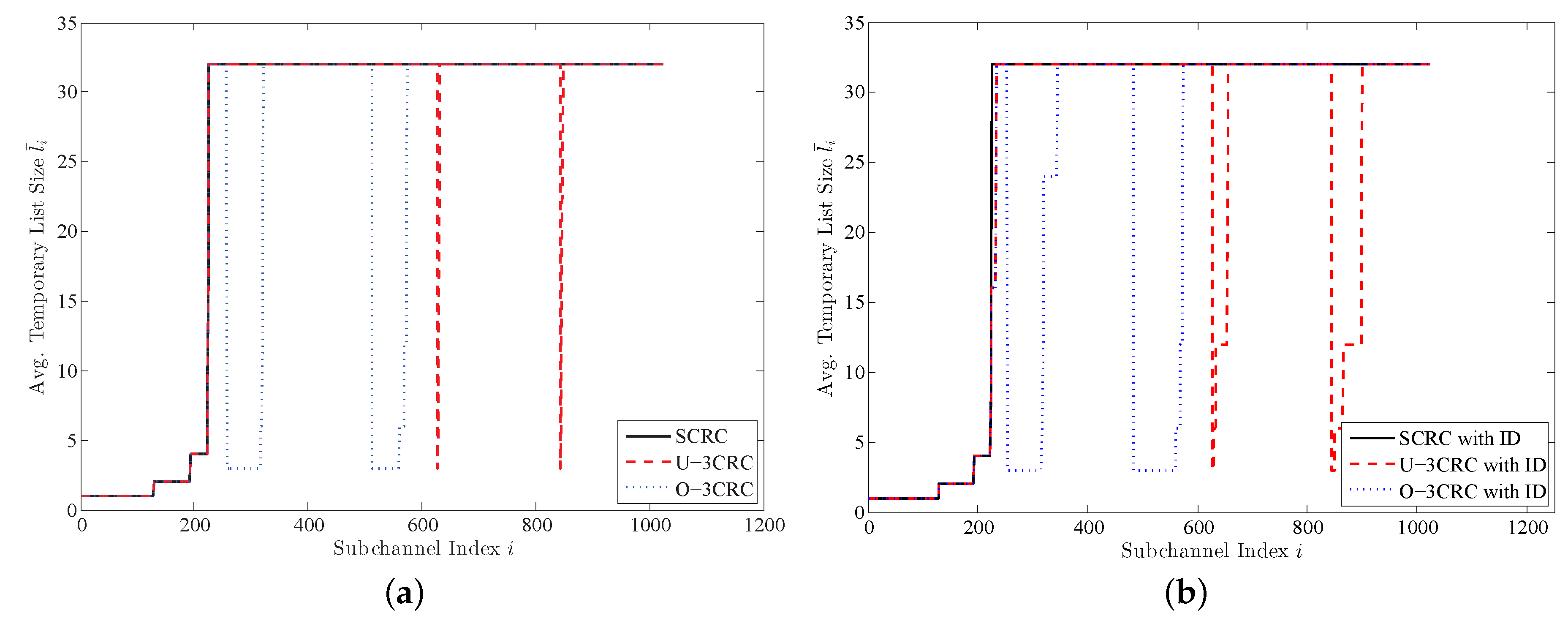
The comparison of the average temporary list sizes between the proposed and conventional 3-CRC schemes for N = 1024 , L = 32 and P = 16 is shown in Figure 4. Figure 4a is under the basic SCL decoding, and Figure 4b under the ID-SCL decoding. For SCRC in Figure 4a, the temporary list size slowly increases up to L until the bit index reaches about 220. In the case of U-3CRC, the average temporary list size decreases from L to 1 + 31 / ( 2 4 ) = 2 . 94 two times due to use of two 4-bit CRC codes. Its temporary list size, however, quickly increases to L again. For the proposed scheme, the temporary list size of O-3CRC is also dropped two times, but the list size is maintained small for a burst of consecutive frozen bits. In Figure 4b, the trend of the temporary list size is similar to that of Figure 4a. However, for O-3CRC, the list size stays small longer due to instant decisions of highly reliable bits on top of frozen operations.
Table 2 and Table 3 show the complexity ratio of the J-tuple CRC schemes to the SCRC scheme with the basic SCL and the ID-SCL decoding. The complexity ratios are estimated by the analysis in Section 3, and the estimation is validated by simulation results. Here, O-2CRC and O-3CRC schemes are optimized for serial and parallel sorters separately. As mentioned, the analysis is done under the assumption that there is no early stopping of decoding that indicates a detected codeword error. This assumption is consistent with a high SNR environment. Thus, the experimental complexity is measured at the high SNR, e.g., E S / N 0 = 1 . 0 , 1 . 5 dB for N = 1024 , 4096 , respectively, by averaging the number of addition-equivalent operations. The complexity ratio from the experiment is in the parentheses of Table 2 and Table 3. It is observed that the experimental values are very close to the estimated ones. Note that the optimization of J-CRC scheme is performed based on the estimated complexity and the estimation turned out to be pretty accurate. By the way, a large complexity reduction of the ID-SCL decoding in Table 3 is obtained due to the skipping of sorting operations.
Figure 5, Figure 6 and Figure 7 give the performance and complexity comparison for the optimized 2-CRC and 3-CRC schemes in a wide range of SNR. The complexity ratio includes the reduction from the early stopping in the low SNR region, and it is calculated based on the complexity of SCRC (under the basic SCL decoding). Only the parallel bitonic sorting is assumed in the scheme optimization and complexity evaluation. The average complexity is obtained via simulation.
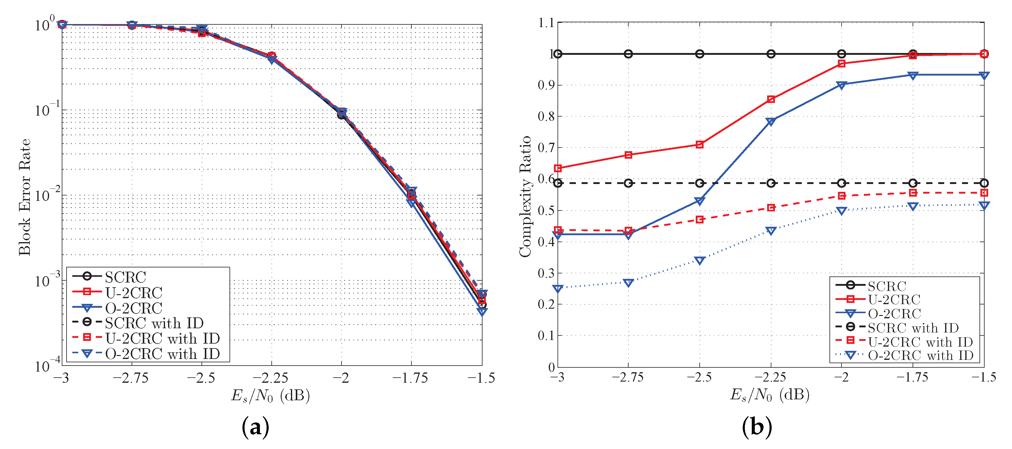
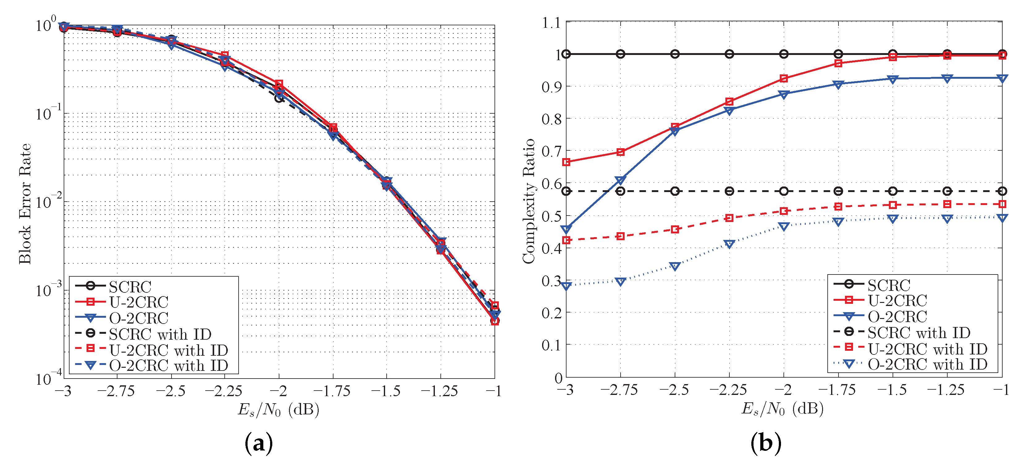
Figure 5 and Figure 6 show the performance and complexity ratio of the proposed and conventional 2-CRC schemes. In Figure 5a and Figure 6a, the negligible performance gap between the proposed and conventional schemes is observed, and the error performance loss is within 0.05 dB. However, Figure 5b and Figure 6b display obvious visible difference in complexity. Especially, when the ID-SCL decoding is applied to the SCRC scheme, about 40% of the complexity is reduced. For N = 1024 , the complexity reduction of O-2CRC under the basic SCL decoding is about 7% points compared to U-2CRC at E S / N 0 = 1 . 0 dB, but when the ID-SCL decoding is used, about 4% points are reduced compared to “U-2CRC with ID”. In addition, at the low SNR, more complexity reduction is acquired thanks to the early stopping. For N = 4096 , the complexity reduction of O-2CRC under the basic SCL decoding is about 22% points compared to U-2CRC at E S / N 0 = 3 . 0 dB, and about 18% points are reduced under the ID-SCL decoding compared to “U-2CRC with ID”.
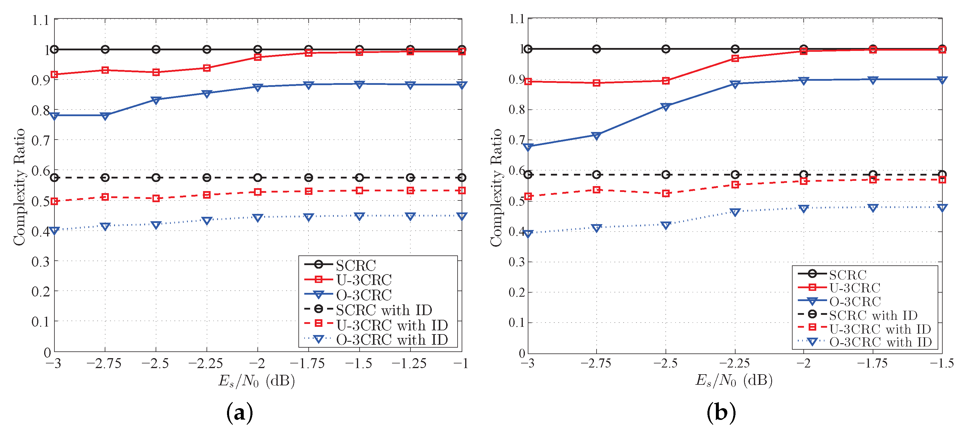
Figure 7 depicts the complexity ratio of the proposed and conventional 3-CRC schemes. The performances for the 3-CRC schemes are not included in this paper because they are virtually the same as for the 2-CRC scheme. For the 3-CRC scheme, the complexity reduction from the early stopping is smaller than the 2-CRC scheme because the CRC of four bits located in the middle of vector u can not eliminate most incorrect paths. Especially, if L = 32 and a CRC of four bits is used, then 32 / ( 2 4 ) = 2 paths survive on average, which implies a lower probability of early decoding termination than the 2-CRC scheme. However, if the ID-SCL decoding is applied, there is more complexity reduction at the high SNR. For N = 1024 , about 12% points (about 9% points) are reduced compared to U-3CRC (U-3CRC with ID), and about 11% points (about 9% points) for N = 4096 compared to U-3CRC (U-3CRC with ID).
Note that, for the proposed J-tuple CRC scheme, the complexity reduction can be increased, while keeping the performance level by selecting A g rigorously, not based on a threshold σ Th . This paper provides a simple and systematic algorithm that minimizes the complexity and performance loss by adjusting the single parameter σ Th .

5. Conclusions

This paper considers a low complexity SCL decoding for polar codes that utilizes multiple CRC codes. In contrast with the other schemes using multiple CRC codes, we define the operational complexity of the SCL decoding in consideration of the hardware implementation, and optimize the CRC positions in terms of the complexity in combination with the ID-SCL decoding. Consequently, the proposed decoding obtains not only the complexity reduction from CRC-based early stopping, but also additional reduction from the reduced number of decoding paths accompanying negligible performance loss. It is also observed that, according to J, there exists a tradeoff in complexity reduction in the low and high SNR regions.

Acknowledgments

This work was supported by the research fund of Signal Intelligence Research Center supervised by Defense Acquisition Program Administration and Agency for Defense Development of Korea. This work was also supported in part by Samsung Electronics (Suwon, Korea).

Author Contributions

Jong-Hwan Kim and Sang-Hyo Kim analyzed decoding complexity, developed the algorithms and wrote the paper; Ji-Woong Jang analyzed implementation complexity of the decoder; Young-Sik Kim designed the experiments and analyzed data. All authors have read and approved the final manuscript.

Conflicts of Interest

The authors declare no conflict of interest. The founding sponsors had no role in the design of the study; in the collection, analyses, or interpretation of data; in the writing of the manuscript, and in the decision to publish the results.

References

  1. Arikan, E. Channel polarization: A method for constructing capacity-achieving codes for symmetric binary-input memoryless channels. IEEE Trans. Inf. Theory 2009, 55, 3051–3073. [Google Scholar] [CrossRef]
  2. Arikan, E. Source polarization. Proccedings of the IEEE International Symposium on Information Theory, Austin, TX, USA, 13–18 June 2010; pp. 899–903. [Google Scholar]
  3. Cronie, H.S.; Korada, S.B. Lossless source coding with polar codes. Proccedings of the IEEE International Symposium on Information Theory, Austin, TX, USA, 13–18 June 2010; pp. 904–908. [Google Scholar]
  4. Korada, S.B.; Urbanke, R.L. Polar codes are optimal for lossy source coding. IEEE Trans. Inf. Theory 2010, 56, 1751–1768. [Google Scholar] [CrossRef]
  5. Abbe, E.; Telatar, E. Polar codes for the m-user multiple access channel. IEEE Trans. Inf. Theory 2012, 58, 5437–5448. [Google Scholar] [CrossRef]
  6. Mahdavifar, H.; El-Khamy, M.; Lee, J.; Kang, I. Achieving the uniform rate region of general multiple access channels by polar coding. IEEE Trans. Commun. 2016, 64, 467–478. [Google Scholar] [CrossRef]
  7. Goela, N.; Abbe, E.; Gastpar, M. Polar codes for broadcast channels. IEEE Trans. Inf. Theory 2015, 61, 758–782. [Google Scholar] [CrossRef]
  8. Mondelli, M.; Hassani, S.H.; Sason, I.; Urbanke, R.L. Achieving Marton’s region for broadcast channels using polar codes. IEEE Trans. Inf. Theory 2015, 61, 783–800. [Google Scholar] [CrossRef]
  9. Hussami, N.; Urbanke, R.L.; Korada, S.B. Performance of polar codes for channel and source coding. Proccedings of the IEEE International Symposium on Information Theory, Seoul, Korea, 28 June–3 July 2009; pp. 1488–1492. [Google Scholar]
  10. Korada, S.B.; Urbanke, R. Polar codes for Slepian–Wolf, Wyner–Ziv, and Gelfand–Pinsker. Proccedings of the IEEE Information Theory Workshop on Information Theory, Cairo, Egypt, 6–8 January 2010; pp. 1–5. [Google Scholar]
  11. Arikan, E. Polar coding for the Slepian–Wolf problem based on monotone chain rules. Proccedings of the IEEE International Symposium on Information Theory, Cambridge, MA, USA, 1–6 July 2012; pp. 566–570. [Google Scholar]
  12. Tal, I.; Vardy, A. List decoding of polar codes. IEEE Trans. Inf. Theory 2015, 61, 2213–2226. [Google Scholar] [CrossRef]
  13. Tal, I.; Vardy, A. List decoding of polar codes. Proccedings of the IEEE International Symposium on Information Theory, St. Petersburg, Russia, 31 July–5 August 2011; pp. 1–5. [Google Scholar]
  14. Wang, T.; Qu, D.; Jiang, T. Parity-check- concatenated polar codes. IEEE Commun. Lett. 2016, 20, 2343–2345. [Google Scholar] [CrossRef]
  15. Wang, R.; Liu, R. A novel puncturing scheme for polar codes. IEEE Commun. Lett. 2014, 18, 2081–2084. [Google Scholar] [CrossRef]
  16. MCC Support. Final Report of 3GPP TSG RAN WG1 #87 v1.0.0 (R1-1701552). In Proceedings of the 3GPP TSG RAN WG1 Meeting #87, Reno, NV, USA, 14–18 November 2016. [Google Scholar]
  17. Yuan, B.; Parhi, K.K. Low-latency successive-cancellation list decoders for polar codes with multibit decision. IEEE Trans. Very Large Scale Integr. Syst. 2015, 23, 2268–2280. [Google Scholar] [CrossRef]
  18. Hung, S.-Y.; Yen, S.-W.; Chen, C.-L.; Chang, H.-C.; Jou, S.-J.; Lee, C.-Y. A 5.7 Gbps row-based layered scheduling LDPC decoder for IEEE 802.15.3c applications. In Proceedings of the IEEE Asian Solid-State Circuits Conference, Beijing, China, 8–10 November 2010. [Google Scholar]
  19. Zhang, Z.; Zhang, L.; Wang, X.; Zhong, C.; Poor, H.V. A split-reduced successive cancellation list decoder for polar codes. IEEE J. Sel. Areas Commun. 2016, 34, 292–302. [Google Scholar] [CrossRef]
  20. Chen, K.; Li, B.; Shen, H.; Jin, J.; Tse, D. Reduce the complexity of list decoding of polar codes by tree-pruning. IEEE Commun. Lett. 2016, 20, 204–207. [Google Scholar] [CrossRef]
  21. Guo, J.; Liu, Z.; Liu, Q. Multi-CRC polar codes and their applications. IEEE Commun. Lett. 2016, 20, 212–215. [Google Scholar] [CrossRef]
  22. Zhou, H.; Zhan, C.; Song, W.; Xu, S.; You, X. Segmented CRC-aided SC list polar decoding. Proccedings of the IEEE Vehicular Technology Conference (VTC Spring), Nanjing, China, 15–18 May 2016. [Google Scholar]
  23. Chiu, M.-C.; Wu, W.-D. Reduced-complexity SCL decoding of multi-CRC-aided polar codes. arXiv, 2016; arXiv:1609.08813. [Google Scholar]
  24. Huawei; HiSilicon. On latency and complexity (R1-164040). In Proceedings of the 3GPP TSG RAN WG1 Meeting #85, Nanjing, China, 23–27 May 2016. [Google Scholar]
  25. Balatsoukas-Stimming, A.; Bastani Parizi, M.; Burg, A. LLR-based successive cancellation list decoding of polar codes. IEEE Trans. Signal. Process. 2015, 63, 5165–5179. [Google Scholar] [CrossRef]
  26. Fossorier, M.; Mihaljevic, M.; Imai, H. Reduced complexity iterative decoding of low-density parity-check codes based on belief propagation. IEEE Trans. Commun. 1999, 47, 673–680. [Google Scholar] [CrossRef]
  27. Leroux, C.; Tal, I.; Vard, A.; Gross, W. Hardware architectures for successive cancellation decoding of polar codes. Proccedings of the IEEE International Conference on Acoustics, Speech and Signal Processing, Prague, Czech, 22–27 May 2011; pp. 1665–1668. [Google Scholar]
  28. Mori, R.; Tanaka, T. Performance of polar codes with the construction using density evolution. IEEE Commun. Lett. 2009, 13, 519–521. [Google Scholar] [CrossRef]
Figure 1. The temporary list size growth in the successive cancellation list (SCL) decoding ( L = 4 ).
Entropy 19 00183 g001
Figure 2. The two node operations for the log-likelihood ratio (LLR) calculation.
Entropy 19 00183 g002
Figure 3. The cyclic redundancy check (CRC) encoding of the J-Tuple CRC scheme.
Entropy 19 00183 g003
Figure 4. The average temporary list size of the proposed and conventional 3-CRC schemes for N = 1024 , L = 32 and P = 16 ; (a) with the basic SCL decoding; (b) with the ID-SCL decoding.
Entropy 19 00183 g004
Figure 5. Comparison of the proposed and conventional 2-CRC schemes for N = 1024 , R = 1 / 2 , L = 32 and P = 16 ; (a) block error rate; (b) complexity ratio.
Entropy 19 00183 g005
Figure 6. Comparison of the proposed and conventional 2-CRC schemes for N = 4096 , R = 1 / 2 , L = 32 and P = 16 ; (a) block error rate; (b) complexity ratio.
Entropy 19 00183 g006
Figure 7. The complexity ratio of the proposed and conventional 3-CRC schemes for R = 1 / 2 , L = 32 and P = 16 ; (a) N = 1024 ; (b) N = 4096 .
Entropy 19 00183 g007
Table 1. The message vector k of the J-tuple CRC schemes for both serial and parallel sorters. The threshold σ Th for the ID-SCL decoding is 10 5 and 5 × 10 8 for N = 1024 , 4096 , respectively.
2-CRC3-CRC
U-2CRCO-2CRCO-2CRC with IDU-3CRCO-3CRCO-3CRC with ID
N = 1024 (256,256)(136,376)(107,405)(170,170,172)(18,118,376)(15,92,405)
N = 4096 (1024,1024)(548,1500)(485,1563)(682,682,684)(79,469,1500)(64,421,1563)
Table 2. The ratio (%) of complexity of the J-CRC scheme (basic SCL decoding) to the SCRC scheme (basic SCL decoding) obtained by analysis and experiment. The experimental values are in parentheses and obtained at E S / N 0 = 1 . 0 , 1 . 5 dB for N = 1024 , 4096 , respectively.
U-2CRCO-2CRCU-3CRCO-3CRC
Sorter TypeSerialParallelSerialParallelSerialParallelSerialParallel
N = 1024 99.6 (99.5)99.5 (99.4)90.4 (90.6)92.6 (92.6)99.3 (99.3)99.2 (99.1)85.6 (85.2)88.9 (88.4)
N = 4096 99.7 (99.5)99.7 (99.8)91.8 (91.7)93.5 (93.3)99.8 (99.7)99.7 (99.7)87.2 (87.3)90.0 (89.9)
Table 3. The ratio (%) of complexity of the J-CRC scheme (ID-SCL decoding) to the SCRC scheme (basic SCL decoding) obtained by analysis and experiment. The experimental values are in parentheses and obtained at E S / N 0 = 1 . 0 , 1 . 5 dB for N = 1024 , 4096 , respectively.
U-2CRCO-2CRCU-3CRCO-3CRC
Sorter TypeSerialParallelSerialParallelSerialParallelSerialParallel
N = 1024 62.7 (62.8)53.3 (53.4)57.3 (57.4)49.2 (49.3)62.9 (62.7)53.5 (53.2)52.0 (51.7)45.1 (44.9)
N = 4096 65.6 (65.7)55.6 (55.7)60.7 (60.6)51.8 (51.8)67.3 (67.3)56.9 (57.0)56.2 (55.9)48.2 (48.1)

