On Hölder Projective Divergences

Abstract

We describe a framework to build distances by measuring the tightness of inequalities and introduce the notion of proper statistical divergences and improper pseudo-divergences. We then consider the Hölder ordinary and reverse inequalities and present two novel classes of Hölder divergences and pseudo-divergences that both encapsulate the special case of the Cauchy–Schwarz divergence. We report closed-form formulas for those statistical dissimilarities when considering distributions belonging to the same exponential family provided that the natural parameter space is a cone (e.g., multivariate Gaussians) or affine (e.g., categorical distributions). Those new classes of Hölder distances are invariant to rescaling and thus do not require distributions to be normalized. Finally, we show how to compute statistical Hölder centroids with respect to those divergences and carry out center-based clustering toy experiments on a set of Gaussian distributions which demonstrate empirically that symmetrized Hölder divergences outperform the symmetric Cauchy–Schwarz divergence.

1. Introduction: Inequality, Proper Divergence and Improper Pseudo-Divergence

1.1. Statistical Divergences from Inequality Gaps

An inequality [1] is denoted mathematically by $\mathrm{lhs}\le \mathrm{rhs}$, where $\mathrm{lhs}$ and $\mathrm{rhs}$ denote respectively the left-hand-side and right-hand-side of the inequality. One can build dissimilarity measures from inequalities $\mathrm{lhs}\le \mathrm{rhs}$ by measuring the inequality tightness: For example, we may quantify the tightness of an inequality by its difference gap:

$$\Delta =\mathrm{rhs}-\mathrm{lhs}\ge 0.$$

(1)

When $\mathrm{lhs}>0$, the inequality tightness can also be gauged by the log-ratio gap:

$$D=log\left(\frac{\mathrm{rhs}}{\mathrm{lhs}}\right)=-log\left(\frac{\mathrm{lhs}}{\mathrm{rhs}}\right)\ge 0.$$

(2)

We may further compose this inequality tightness value measuring non-negative gaps with a strictly monotonically increasing function f (with $f(0)=0$).

A bi-parametric inequality $\mathrm{lhs}(p,q)\le \mathrm{rhs}(p,q)$ is called proper if it is strict for $p\ne q$ (i.e., $\mathrm{lhs}(p,q)<\mathrm{rhs}(p,q),\forall p\ne q$) and tight if and only if (iff) $p=q$ (i.e., $\mathrm{lhs}(p,q)=\mathrm{rhs}(p,q),\forall p=q$). Thus a proper bi-parametric inequality allows one to define dissimilarities such that $D(p,q)=0$ iff $p=q$. Such a dissimilarity is called proper. Otherwise, an inequality or dissimilarity is said to be improper. Note that there are many equivalent words used in the literature instead of (dis-)similarity: distance (although often assumed to have metric properties; here, we used the notion of distance as a dissimilarity that may be asymmetric), pseudo-distance, discrimination, proximity, information deviation, etc.

A statistical dissimilarity between two discrete or continuous distributions $p(x)$ and $q(x)$ on a support $\mathcal{X}$ can thus be defined from inequalities by summing up or taking the integral for the inequalities instantiated on the observation space $\mathcal{X}$:

$$\begin{array}{cc}\hfill \forall x\in \mathcal{X},& D_x(p,q)=\mathrm{rhs}(p(x),q(x))-\mathrm{lhs}(p(x),q(x))\Rightarrow \hfill \\ & D(p,q)=\left\{\begin{array}{cc}{\sum }_{x\in \mathcal{X}}\left[\mathrm{rhs}(p(x),q(x))-\mathrm{lhs}(p(x),q(x))\right]\hfill & \mathrm{discrete}\mathrm{case},\hfill \\ {\int }_{\mathcal{X}}\left[\mathrm{rhs}(p(x),q(x))-\mathrm{lhs}(p(x),q(x))\right]\mathrm{d}x\hfill & \mathrm{continuous}\mathrm{case}.\hfill \end{array}\right.\hfill \end{array}$$

(3)

In such a case, we get a separable divergence by construction. Some non-separable inequalities induce a non-separable divergence. For example, the renowned Cauchy–Schwarz divergence [2] is not separable because in the inequality:

$${\int }_{\mathcal{X}}p(x)q(x)\mathrm{d}x\le \sqrt{\left({\int }_{\mathcal{X}}p{(x)}^2\mathrm{d}x\right)\left({\int }_{\mathcal{X}}q{(x)}^2\mathrm{d}x\right)},$$

(4)

the rhs is not separable.

Furthermore, a proper dissimilarity is called a divergence in information geometry [3] when it is $C^3$ (i.e., three times differentiable, thus allowing one to define a metric tensor [4] and a cubic tensor [3]).

Many familiar distances can be reinterpreted as inequality gaps in disguise. For example, Bregman divergences [5] and Jensen divergences [6] (also called Burbea–Rao divergences [7,8]) can be reinterpreted as inequality difference gaps and the Cauchy–Schwarz distance [2] as an inequality log-ratio gap:

Example 1 (Bregman divergence as a Bregman score-induced gap divergence).

A proper score function [9] $S(p:q)$ induces a gap divergence $D(p:q)=S(p:q)-S(p:p)\ge 0$. A Bregman divergence [5] $B_F(p:q)$ for a strictly convex and differentiable real-valued generator $F(x)$ is induced by the Bregman score $S_F(p:q)$. Let $S_F(p:q)=-F(q)-\langle p-q,\nabla F(q)\rangle$ denote the Bregman proper score minimized for $p=q$. Then, the Bregman divergence is a gap divergence: $B_F(p:q)=S_F(p:q)-S_F(p:p)\ge 0$. When F is strictly convex, the Bregman score is proper, and the Bregman divergence is proper.

Example 2 (Cauchy–Schwarz distance as a log-ratio gap divergence).

Consider the Cauchy–Schwarz inequality ${\int }_{\mathcal{X}}p(x)q(x)\mathrm{d}x\le \sqrt{\left({\int }_{\mathcal{X}}p{(x)}^2\mathrm{d}x\right)\left({\int }_{\mathcal{X}}q{(x)}^2\mathrm{d}x\right)}$. Then, the Cauchy–Schwarz distance [2] between two continuous distributions is defined by $\mathrm{CS}(p:q)=-log\frac{{\int }_{\mathcal{X}}p(x)q(x)\mathrm{d}x}{\sqrt{({\int }_{\mathcal{X}}p{(x)}^2\mathrm{d}x)({\int }_{\mathcal{X}}q{(x)}^2\mathrm{d}x)}}\ge 0$.

Note that we use the modern notation $D(p:q)$ to emphasize that the divergence is potentially asymmetric: $D(p:q)\ne D(q:p)$; see [3]. In information theory [10], the older notation “$\parallel$” is often used instead of the “:” that is used in information geometry [3].

To conclude this introduction, let us finally introduce the notion of projective statistical distances. A statistical distance $D(p:q)$ is said to be projective when it is invariant to scaling of $p(x)$ and $q(x)$, that is,

$$D(\lambda p:{\lambda }^{\prime }q)=D(p:q),\forall \lambda ,{\lambda }^{\prime }>0.$$

(5)

The Cauchy–Schwarz distance is a projective divergence. Another example of such a projective divergence is the parametric γ-divergence [11].

Example 3 (γ-divergence as a projective score-induced gap divergence).

The γ-divergence [11,12] $D_{\gamma }(p:q)$ for $\gamma >0$ is projective:

$$\begin{array}{cc}\hfill D_{\gamma }(p:q)& =S_{\gamma }(p:q)-S_{\gamma }(p:p),with\hfill \\ \hfill S_{\gamma }(p:q)& =-\frac{1}{\gamma (1+\gamma )}\frac{\int p(x)q{(x)}^{\gamma }\mathrm{d}x}{{\left(\int q{(x)}^{1+\gamma }\mathrm{d}x\right)}^{\frac{\gamma }{1+\gamma }}}.\hfill \end{array}$$

The γ-divergence is related to the proper pseudo-spherical score [11].

The γ-divergences have been proven useful for robust statistical inference [11] in the presence of heavy outlier contamination. In general, bi-parametric homogeneous inequalities yield corresponding log-ratio projective divergences: Let $\mathrm{lhs}(p:q)$ and $\mathrm{rhs}(p:q)$ be homogeneous functions of degree $k\in \mathbb{N}$ (i.e., $\mathrm{lhs}(\lambda p:{\lambda }^{\prime }q)={(\lambda {\lambda }^{\prime })}^k\mathrm{lhs}(p:q)$ and $\mathrm{rhs}(\lambda p:{\lambda }^{\prime }q)={(\lambda {\lambda }^{\prime })}^k\mathrm{rhs}(p:q)$); then, it comes that:

$$D(\lambda p:{\lambda }^{\prime }q)=-log\left(\frac{\mathrm{lhs}(\lambda p:{\lambda }^{\prime }q)}{\mathrm{rhs}(\lambda p:{\lambda }^{\prime }q)}\right)=-log\left(\frac{{(\lambda {\lambda }^{\prime })}^k\mathrm{lhs}(p:q)}{{(\lambda {\lambda }^{\prime })}^k\mathrm{rhs}(p:q)}\right)=-log\left(\frac{\mathrm{lhs}(p:q)}{\mathrm{rhs}(p:q)}\right)=D(p:q).$$

(6)

For example, Hölder and Cauchy–Schwarz inequalities are homogeneous inequalities of degree one that yield projective log-ratio divergences.

There are many works studying classes of (statistical) divergences and their properties. For example, Zhang [13] studied the relationships between divergences, duality and convex analysis by defining the class of divergences:

$$D_F^{(\alpha )}(p:q)=\frac{4}{1-{\alpha }^2}\left(\frac{1-\alpha }{2}F(p)+\frac{1+\alpha }{2}F(q)-F\left(\frac{1-\alpha }{2}p+\frac{1+\alpha }{2}q\right)\right),\alpha \ne 1,$$

(7)

for a real-valued convex generator function F. Interestingly, this divergence can be interpreted as a gap divergence derived from the Jensen convex inequality:

$$\frac{1-\alpha }{2}F(p)+\frac{1+\alpha }{2}F(q)\ge F\left(\frac{1-\alpha }{2}p+\frac{1+\alpha }{2}q\right).$$

(8)

This work is further extended in [14] where Zhang stresses the two different types of duality in information geometry: the referential duality and the representational duality (with the study of the $(\rho ,\tau )$-geometry for monotone embeddings).

It is well-known that Rényi divergence generalizes the Kullback–Leibler divergence: Rényi divergence is induced by Rényi entropy, which generalizes Shannon entropy, while keeping the important feature of being additive. Another generalization of Shannon entropy is Tsallis entropy, which is non-additive in general and allows one to define the Tsallis divergence. Both the Rényi and Tsallis entropies can be unified by the biparametric family of Sharma–Mittal entropies [15], and the corresponding Sharma–Mittal divergences can be defined. There are many ways to extend the definitions of Sharma–Mittal divergences. For example, in [16], a generalization of Rényi divergences is proposed, and its induced geometry is investigated.

1.2. Pseudo-Divergences and the Axiom of Indiscernibility

Consider a broader class of statistical pseudo-divergences based on improper inequalities, where the tightness of an inequality $\mathrm{lhs}(p,q)\le \mathrm{rhs}(p,q)$ does not imply that $p=q$. This family of dissimilarity measures has interesting properties that have not been studied before.

Formally, statistical pseudo-divergences are defined with respect to density measures $p(x)$ and $q(x)$ with $x\in \mathcal{X}$, where $\mathcal{X}$ denotes the support. By definition, pseudo-divergences satisfy the following three fundamental properties:

• Non-negativeness: $D(p:q)\ge 0$ for any $p(x),q(x)$;
• Reachable indiscernibility:

  • $\forall p(x)$, there exists $q(x)$, such that $D(p:q)=0$,
  • $\forall q(x)$, there exists $p(x)$, such that $D(p:q)=0$.
• Positive correlation: if $D(p:q)=0$, then $\left(p(x_1)-p(x_2)\right)\left(q(x_1)-q(x_2)\right)\ge 0$ for any $x_1$, $x_2\in \mathcal{X}$.

As compared to statistical divergence measures, such as the Kullback–Leibler (KL) divergence:

$$\mathrm{KL}(p:q)={\int }_{\mathcal{X}}p(x)log\frac{p(x)}{q(x)}\mathrm{d}x,$$

(9)

pseudo-divergences do not require $D(p:p)=0$. Instead, any pair of distributions $p(x)$ and $q(x)$ with $D(p:q)=0$ only have to be “positively correlated” such that $p(x_1)\le p(x_2)$ implies $q(x_1)\le q(x_2)$, and vice versa. Any divergence with $D(p:q)=0\Rightarrow p(x)=q(x)$ (law of indiscernibles) automatically satisfies this weaker condition, and therefore, any divergence belongs to the broader class of pseudo-divergences. Indeed, if $p(x)=q(x)$, then $(p(x_1)-p(x_2))(q(x_1)-q(x_2))={(p(x_1)-p(x_2))}^2\ge 0$. However, the converse is not true. As we shall describe in the remainder, the family of pseudo-divergences is not limited to proper divergence measures. In the remainder, the term “pseudo-divergence” refers to such divergences that are not proper divergence measures.

We study two novel statistical dissimilarity families: one family of statistical improper pseudo-divergences and one family of proper statistical divergences. Within the class of pseudo-divergences, this work concentrates on defining a tri-parametric family of dissimilarities called Hölder log-ratio gap divergence that we concisely abbreviate as HPD for “Hölder pseudo divergence” in the remainder. We also study its proper divergence counterpart termed HD for “Hölder divergence”.

1.3. Prior Work and Contributions

The term “Hölder divergence” was first coined in 2014 based on the definition of the Hölder score [17,18]: The score-induced Hölder divergence $D(p:q)$ is a proper gap divergence that yields a scale-invariant divergence. Let $p_{a,\sigma }(x)=a\sigma p(\sigma x)$ for $a,\sigma >0$ be a transformation. Then, a scale-invariant divergence satisfies $D(p_{a,\sigma }:q_{a,\sigma })=\kappa (a,\sigma )D(p:q)$ for a function $\kappa (a,\sigma )>0$. This gap divergence is proper since it is based on the so-called Hölder score, but is not projective and does not include the Cauchy–Schwarz divergence. Due to these differences, the Hölder log-ratio gap divergence introduced here shall not be confused with the Hölder gap divergence induced by the Hölder score that relies both on a scalar γ and a function $\varphi (·)$.

We shall introduce two novel families of log-ratio projective gap divergences based on Hölder ordinary (or forward) and reverse inequalities that extend the Cauchy–Schwarz divergence, study their properties and consider as an application clustering Gaussian distributions: We experimentally show better clustering results when using symmetrized Hölder divergences than using the Cauchy–Schwarz divergence. To contrast with the “Hölder composite score-induced divergences” of [18], our Hölder divergences admit closed-form expressions between distributions belonging to the same exponential families [19] provided that the natural parameter space is a cone or affine.

Our main contributions are summarized as follows:

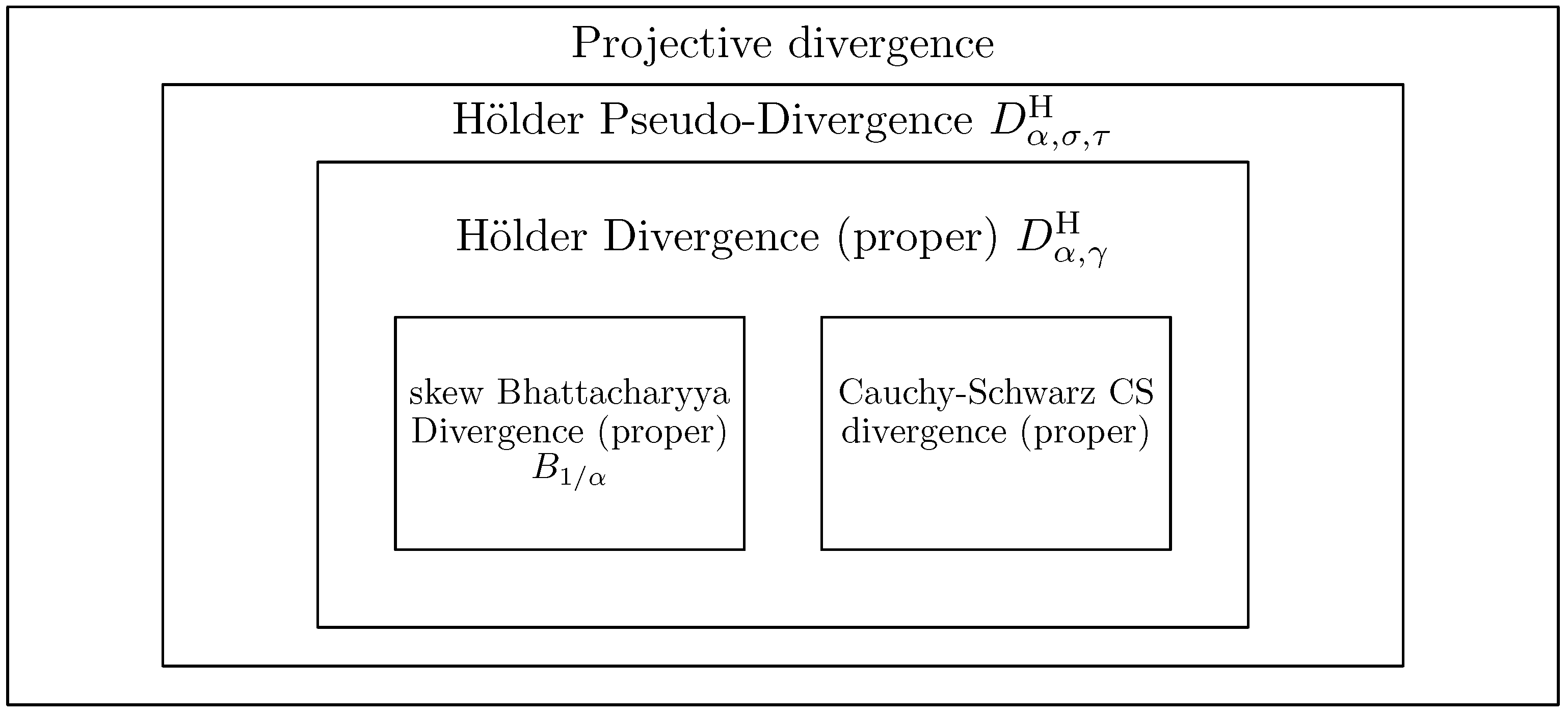
• Define the tri-parametric family of Hölder improper pseudo-divergences (HPDs) in Section 2 and the bi-parametric family of Hölder proper divergences in Section 3 (HDs) for positive and probability measures, and study their properties (including their relationships with skewed Bhattacharyya distances [8] via escort distributions);
• Report closed-form expressions of those divergences for exponential families when the natural parameter space is a cone or affine (including, but not limited to the cases of categorical distributions and multivariate Gaussian distributions) in Section 4;
• Provide approximation techniques to compute those divergences between mixtures based on log-sum-exp inequalities in Section 4.6;
• Describe a variational center-based clustering technique based on the convex-concave procedure for computing Hölder centroids, and report our experimental results in Section 5.

1.4. Organization

This paper is organized as follows: Section 2 introduces the definition and properties of Hölder pseudo-divergences (HPDs). It is followed by Section 3 that describes Hölder proper divergences (HDs). In Section 4, closed-form expressions for those novel families of divergences are reported for the categorical, multivariate Gaussian, Bernoulli, Laplace and Wishart distributions. Section 5 defines Hölder statistical centroids and presents a variational k-means clustering technique: we show experimentally that using Hölder divergences improves clustering quality over the Cauchy–Schwarz divergence. Finally, Section 6 concludes this work and hints at further perspectives from the viewpoint of statistical estimation and manifold learning. In Appendix A, we recall the proof of the ordinary and reverse Hölder’s inequalities.

2. Hölder Pseudo-Divergence: Definition and Properties

Hölder’s inequality (see [20,21] and Appendix A for a proof) states for positive real-valued functions $p(x)$ and $q(x)$ defined on the support $\mathcal{X}$ that:

$${\int }_{\mathcal{X}}p(x)q(x)\mathrm{d}x\le {\left({\int }_{\mathcal{X}}p{(x)}^{\alpha }\mathrm{d}x\right)}^{\frac{1}{\alpha }}{\left({\int }_{\mathcal{X}}q{(x)}^{\beta }\mathrm{d}x\right)}^{\frac{1}{\beta }},$$

(10)

where exponents α and β satisfy $\alpha \beta >0$, as well as the exponent conjugacy condition: $\frac{1}{\alpha }+\frac{1}{\beta }=1$. In a more general form, Hölder’s inequality holds for any real and complex valued functions. In this work, we only focus on real positive functions that are densities of positive measures. We also write $\beta =\overline{\alpha }=\frac{\alpha }{\alpha -1}$, meaning that α and β are conjugate Hölder exponents. We check that $\alpha >1$ and $\beta >1$. Hölder inequality holds even if the lhs is infinite (meaning that the integral diverges), since the rhs is also infinite in that case.

The reverse Hölder inequality holds for conjugate exponents $\frac{1}{\alpha }+\frac{1}{\beta }=1$ with $\alpha \beta <0$ (then $0<\alpha <1$ and $\beta <0$, or $\alpha <0$ and $0<\beta <1$):

$${\int }_{\mathcal{X}}p(x)q(x)\mathrm{d}x\ge {\left({\int }_{\mathcal{X}}p{(x)}^{\alpha }\mathrm{d}x\right)}^{\frac{1}{\alpha }}{\left({\int }_{\mathcal{X}}q{(x)}^{\beta }\mathrm{d}x\right)}^{\frac{1}{\beta }}.$$

(11)

Both Hölder’s inequality and the reverse Hölder inequality turn tight when $p{(x)}^{\alpha }\propto q{(x)}^{\beta }$ (see proof in Appendix A).

2.1. Definition

Let $(\mathcal{X},\mathcal{F},\mu )$ be a measurable space where μ is the Lebesgue measure, and let $L^{\gamma }(\mathcal{X},\mu )$ denote the Lebesgue space of functions that have their γ-th power of absolute value Lebesgue integrable, for any $\gamma >0$ (when $\gamma \ge 1$, $L^{\gamma }(\mathcal{X},\mu )$ is a Banach space). We define the following pseudo-divergence:

Definition 1 (Hölder statistical pseudo-divergence).

For conjugate exponents α and β with $\alpha \beta >0$ and $\sigma ,\tau >0$, the Hölder pseudo-divergence (HPD) between two densities $p(x)\in L^{\alpha \sigma }(\mathcal{X},\mu )$ and $q(x)\in L^{\beta \tau }(\mathcal{X},\mu )$ of positive measures absolutely continuous with respect to (w.r.t.) μ is defined by the following log-ratio gap:

$$D_{\alpha ,\sigma ,\tau }^{\mathtt{H}}(p:q)=-log\left(\frac{{\int }_{\mathcal{X}}p{(x)}^{\sigma }q{(x)}^{\tau }\mathrm{d}x}{{\left({\int }_{\mathcal{X}}p{(x)}^{\alpha \sigma }\mathrm{d}x\right)}^{\frac{1}{\alpha }}{\left({\int }_{\mathcal{X}}q{(x)}^{\beta \tau }\mathrm{d}x\right)}^{\frac{1}{\beta }}}\right).$$

(12)

When $0<\alpha <1$ and $\beta =\overline{\alpha }=\frac{\alpha }{\alpha -1}<0$, or $\alpha <0$ and $0<\beta <1$, and $\sigma ,\tau >0$, the reverse HPD is defined by:

$$D_{\alpha ,\sigma ,\tau }^{\mathtt{H}}(p:q)=log\left(\frac{{\int }_{\mathcal{X}}p{(x)}^{\sigma }q{(x)}^{\tau }\mathrm{d}x}{{\left({\int }_{\mathcal{X}}p{(x)}^{\alpha \sigma }\mathrm{d}x\right)}^{\frac{1}{\alpha }}{\left({\int }_{\mathcal{X}}q{(x)}^{\beta \tau }\mathrm{d}x\right)}^{\frac{1}{\beta }}}\right).$$

(13)

By Hölder’s inequality and the reverse Hölder inequality, $D_{\alpha ,\sigma ,\tau }^{\mathtt{H}}(p:q)\ge 0$ with $D_{\alpha ,\sigma ,\tau }^{\mathtt{H}}(p:q)=0$ iff $p{(x)}^{\alpha \sigma }\propto {q(x)}^{\beta \tau }$ or equivalently $q(x)\propto {p(x)}^{\frac{\alpha \sigma }{\beta \tau }}=p{(x)}^{\frac{\sigma }{\tau }(\alpha -1)}$. When $\alpha >1$, $x^{\frac{\sigma }{\tau }(\alpha -1)}$ is monotonically increasing, and $D_{\alpha ,\sigma ,\tau }^{\mathtt{H}}$ is indeed a pseudo-divergence. However, the reverse HPD is not a pseudo-divergence because $x^{\frac{\sigma }{\tau }(\alpha -1)}$ will be monotonically decreasing if $\alpha <0$ or $0<\alpha <1$. Therefore, we only consider HPD with $\alpha >1$ in the remainder, and leave here the notion of reverse Hölder divergence for future studies.

When $\alpha =\beta =2$, $\sigma =\tau =1$, the HPD becomes the Cauchy–Schwarz divergence $\mathrm{CS}$ [22]:

$$D_{2,1,1}^{\mathtt{H}}(p:q)=\mathrm{CS}(p:q)=-log\left(\frac{{\int }_{\mathcal{X}}p(x)q(x)\mathrm{d}x}{{\left({\int }_{\mathcal{X}}p{(x)}^2\mathrm{d}x\right)}^{\frac{1}{2}}{\left({\int }_{\mathcal{X}}q{(x)}^2\mathrm{d}x\right)}^{\frac{1}{2}}}\right),$$

(14)

which has been proven useful to get closed-form divergence formulas between mixtures of exponential families with conic or affine natural parameter spaces [23].

The Cauchy–Schwarz divergence is proper for probability densities since the Cauchy–Schwarz inequality becomes an equality iff $q(x)=\lambda p{(x)}^{\frac{\sigma }{\tau }(\alpha -1)}=\lambda p(x)$ implying that $\lambda ={\int }_{\mathcal{X}}\lambda p(x)\mathrm{d}x={\int }_{\mathcal{X}}q(x)\mathrm{d}x=1$. It is however not proper for positive densities.

Fact 1 (CS is only proper for probability densities).

The Cauchy–Schwarz divergence $\mathrm{CS}(p:q)$ is proper for square-integrable probability densities $p(x),q(x)\in L^2(\mathcal{X},\mu )$, but not proper for positive square-integrable densities.

2.2. Properness and Improperness

In the general case, the divergence $D_{\alpha ,\sigma ,\tau }^{\mathtt{H}}$ is not even proper for normalized (probability) densities, not to mention general unnormalized (positive) densities. Indeed, when $p(x)=q(x)$, we have:

$$D_{\alpha ,\sigma ,\tau }^{\mathtt{H}}(p:p)=-log\left(\frac{\int p{(x)}^{\sigma +\tau }\mathrm{d}x}{{\left(\int p{(x)}^{\alpha \sigma }\mathrm{d}x\right)}^{\frac{1}{\alpha }}{\left(\int p{(x)}^{\beta \tau }\mathrm{d}x\right)}^{\frac{1}{\beta }}}\right)\ne 0\mathrm{when}\alpha \sigma \ne \beta \tau .$$

(15)

Let us consider the general case. For unnormalized positive distributions $\tilde{p}(x)$ and $\tilde{q}(x)$ (the tilde notation stems from the notation of homogeneous coordinates in projective geometry), the inequality becomes an equality when: $\tilde{p}{(x)}^{\alpha \sigma }\propto \tilde{q}{(x)}^{\beta \tau }$, i.e., $p{(x)}^{\alpha \sigma }\propto {q(x)}^{\beta \tau }$, or $q(x)\propto {p(x)}^{\alpha \sigma /\overline{\alpha }\tau }=p{(x)}^{\frac{\sigma }{\tau }(\alpha -1)}$. We can check that $D_{\alpha ,\sigma ,\tau }^{\mathtt{H}}(p:\lambda p^{\frac{\sigma }{\tau }(\alpha -1)})=0$ for any $\lambda >0$:

$$-log\left(\frac{\int p{(x)}^{\sigma }{\lambda }^{\tau }p{(x)}^{\sigma (\alpha -1)}\mathrm{d}x}{{\left(\int p{(x)}^{\alpha \sigma }\mathrm{d}x\right)}^{\frac{1}{\alpha }}{\left(\int {\lambda }^{\beta \tau }p{(x)}^{(\alpha -1)\beta \sigma }\mathrm{d}x\right)}^{\frac{1}{\beta }}}\right)=-log\left(\frac{\int {\lambda }^{\tau }p{(x)}^{\alpha \sigma }\mathrm{d}x}{{\left(\int p{(x)}^{\alpha \sigma }\mathrm{d}x\right)}^{\frac{1}{\alpha }}{\left(\int {\lambda }^{\beta \tau }p{(x)}^{\alpha \sigma }\mathrm{d}x\right)}^{\frac{1}{\beta }}}\right)=0,$$

(16)

since $(\alpha -1)\beta =(\alpha -1)\overline{\alpha }=(\alpha -1)\frac{\alpha }{\alpha -1}=\alpha$.

Fact 2 (HPD is improper).

The Hölder pseudo-divergences are improper statistical distances.

2.3. Reference Duality

In general, Hölder divergences are asymmetric when $\alpha \ne \beta$ ($\ne 2$) or $\sigma \ne \tau$, but enjoy the following reference duality [24]:

$$D_{\alpha ,\sigma ,\tau }^{\mathtt{H}}(p:q)=D_{\beta ,\tau ,\sigma }^{\mathtt{H}}(q:p)=D_{\frac{\alpha }{\alpha -1},\tau ,\sigma }^{\mathtt{H}}(q:p).$$

(17)

Fact 3 (Reference duality HPD).

The Hölder pseudo-divergences satisfy the reference duality $\beta =\overline{\alpha }=\frac{\alpha }{\alpha -1}$: $D_{\alpha ,\sigma ,\tau }^{\mathtt{H}}(p:q)=D_{\beta ,\tau ,\sigma }^{\mathtt{H}}(q:p)=D_{\frac{\alpha }{\alpha -1},\tau ,\sigma }^{\mathtt{H}}(q:p)$.

An arithmetic symmetrization of the HPD yields a symmetric HPD $S_{\alpha ,\sigma ,\tau }^{\mathtt{H}}$, given by:

$$\begin{array}{ccc}\hfill S_{\alpha ,\sigma ,\tau }^{\mathtt{H}}(p:q)& =& S_{\alpha ,\sigma ,\tau }^{\mathtt{H}}(q:p)=\frac{D_{\alpha ,\sigma ,\tau }^{\mathtt{H}}(p:q)+D_{\alpha ,\sigma ,\tau }^{\mathtt{H}}(q:p)}{2},\hfill \\ & =& -\frac{1}{2}log\left(\frac{\int p{(x)}^{\sigma }q{(x)}^{\tau }\mathrm{d}x\int p{(x)}^{\tau }q{(x)}^{\sigma }\mathrm{d}x}{{\left(\int p{(x)}^{\alpha \sigma }\mathrm{d}x\right)}^{\frac{1}{\alpha }}{\left(\int p{(x)}^{\beta \tau }\mathrm{d}x\right)}^{\frac{1}{\beta }}{\left(\int q{(x)}^{\alpha \sigma }\mathrm{d}x\right)}^{\frac{1}{\alpha }}{\left(\int q{(x)}^{\beta \tau }\mathrm{d}x\right)}^{\frac{1}{\beta }}}\right).\hfill \end{array}$$

(18)

2.4. HPD is a Projective Divergence

In the above definition, densities $p(x)$ and $q(x)$ can either be positive or normalized probability distributions. Let $\tilde{p}(x)$ and $\tilde{q}(x)$ denote positive (not necessarily normalized) measures, and $w(\tilde{p})={\int }_{\mathcal{X}}\tilde{p}(x)\mathrm{d}x$ the overall mass so that $p(x)=\frac{\tilde{p}(x)}{w(\tilde{p})}$ is the corresponding normalized probability measure. Then, we check that HPD is a projective divergence [11] since:

$$D_{\alpha ,\sigma ,\tau }^{\mathtt{H}}(\tilde{p}:\tilde{q})=D_{\alpha ,\sigma ,\tau }^{\mathtt{H}}(p:q),$$

(19)

or in general:

$$D_{\alpha ,\sigma ,\tau }^{\mathtt{H}}(\lambda p:{\lambda }^{\prime }q)=D_{\alpha ,\sigma ,\tau }^{\mathtt{H}}(p:q)$$

(20)

for all prescribed constants $\lambda ,{\lambda }^{\prime }>0$. Projective divergences may also be called “angular divergences” or “cosine divergences”, since they do not depend on the total mass of the density measures.

Fact 4 (HPD is projective).

The Hölder pseudo-divergences are projective distances.

2.5. Escort Distributions and Skew Bhattacharyya Divergences

Let us define with respect to the probability measures $p(x)\in L^{\frac{1}{\alpha }}(\mathcal{X},\mu )$ and $q(x)\in L^{\frac{1}{\beta }}(\mathcal{X},\mu )$ the following escort probability distributions [3]:

$$p_{\alpha }^E(x)=\frac{p{(x)}^{\frac{1}{\alpha }}}{\int p{(x)}^{\frac{1}{\alpha }}\mathrm{d}x},$$

(21)

and

$$q_{\beta }^E(x)=\frac{q{(x)}^{\frac{1}{\beta }}}{\int q{(x)}^{\frac{1}{\beta }}\mathrm{d}x}.$$

(22)

Since HPD is a projective divergence, we compute with respect to the conjugate exponents α and β the Hölder escort divergence (HED):

$$D_{\alpha }^{\mathrm{HE}}(p:q)=D_{\alpha ,1,1}^{\mathtt{H}}(p_{\alpha }^E:q_{\beta }^E)=D_{\alpha ,\frac{1}{\alpha },\frac{1}{\beta }}^{\mathtt{H}}(p:q)=-log{\int }_{\mathcal{X}}p{(x)}^{1/\alpha }q{(x)}^{1/\beta }\mathrm{d}x=B_{1/\alpha }(p:q),$$

(23)

which turns out to be the familiar skew Bhattacharyya divergence $B_{1/\alpha }(p:q)$; see [8].

Fact 5 (HED as a skew Bhattacharyya divergence).

The Hölder escort divergence amounts to a skew Bhattacharyya divergence: $D_{\alpha }^{\mathrm{HE}}(p:q)=B_{1/\alpha }(p:q)$ for any $\alpha >0$.

In particular, the Cauchy–Schwarz escort divergence ${\mathrm{CS}}^{\mathrm{HE}}(p:q)$ amounts to the Bhattacharyya distance [25] $B(p:q)=-log{\int }_{\mathcal{X}}\sqrt{p(x)q(x)}\mathrm{d}x$:

$${\mathrm{CS}}^{\mathrm{HE}}(p:q)=D_2^{\mathrm{HE}}(p:q)=D_{2,1,1}^{\mathtt{H}}(p_2^E:q_2^E)=D_{2,\frac{1}{2},\frac{1}{2}}^{\mathtt{H}}(p:q)=B_{1/2}(p:q)=B(p:q).$$

(24)

Observe that the Cauchy–Schwarz escort distributions are the square root density representations [26] of distributions.

3. Proper Hölder Divergence

3.1. Definition

To get a proper HD between probability distributions $p(x)$ and $q(x)$, we need to have $p{(x)}^{\alpha \sigma }\propto q{(x)}^{\beta \tau }$. That is, we have $\alpha \sigma =\beta \tau$, or equivalently, we set $\tau =(\alpha -1)\sigma$ for free prescribed parameters $\alpha >1$ and $\sigma >0$. Alternatively, as we shall consider in the remainder, one may set $\alpha \sigma =\beta \tau =\gamma$ as a free prescribed parameter, which yields $\sigma =\gamma /\alpha$ and $\tau =\gamma /\beta$. Thus, in general, we define a bi-parametric family of proper Hölder divergence on probability distributions $D_{\alpha ,\gamma }^{\mathtt{H}}$.

Let $p(x)$ and $q(x)$ be positive measures in $L^{\gamma }(\mathcal{X},\mu )$ for a prescribed scalar value $\gamma >0$. Plugging $\sigma =\gamma /\alpha$ and $\tau =\gamma /\beta$ into the definition of HPD $D_{\alpha ,\sigma ,\tau }^{\mathtt{H}}$, we get the following definition:

Definition 2 (Proper Hölder divergence).

For conjugate exponents $\alpha ,\beta >0$ and $\gamma >0$, the proper Hölder divergence (HD) between two densities $p(x)$ and $q(x)$ is defined by:

$$D_{\alpha ,\gamma }^{\mathtt{H}}(p:q)=D_{\alpha ,\frac{\gamma }{\alpha },\frac{\gamma }{\beta }}^{\mathtt{H}}(p:q)=-log\left(\frac{{\int }_{\mathcal{X}}p{(x)}^{\gamma /\alpha }q{(x)}^{\gamma /\beta }\mathrm{d}x}{{({\int }_{\mathcal{X}}p{(x)}^{\gamma }\mathrm{d}x)}^{1/\alpha }{({\int }_{\mathcal{X}}q{(x)}^{\gamma }\mathrm{d}x)}^{1/\beta }}\right).$$

(25)

Following Hölder’s inequality, we can check that $D_{\alpha ,\gamma }^{\mathtt{H}}(p:q)\ge 0$ and $D_{\alpha ,\gamma }^{\mathtt{H}}(p:q)=0$ iff $p{(x)}^{\gamma }\propto q{(x)}^{\gamma }$, i.e., $p(x)\propto q(x)$ (see Appendix A). If $p(x)$ and $q(x)$ belong to the statistical probability manifold, then $D_{\alpha ,\gamma }^{\mathtt{H}}(p:q)=0$ iff $p(x)=q(x)$ almost everywhere. This says that HD is a proper divergence for probability measures, and it becomes a pseudo-divergence for positive measures. Note that we have abused the notation $D^{\mathtt{H}}$ to denote both the Hölder pseudo-divergence (with three subscripts) and the Hölder divergence (with two subscripts).

Similar to HPD, HD is asymmetric when $\alpha \ne \beta$ with the following reference duality:

$$D_{\alpha ,\gamma }^{\mathtt{H}}(p:q)=D_{\overline{\alpha },\gamma }^{\mathtt{H}}(q:p).$$

(26)

HD can be symmetrized as:

$$S_{\alpha ,\gamma }^{\mathtt{H}}(p:q)=\frac{D_{\alpha ,\gamma }^{\mathtt{H}}(p:q)+D_{\alpha ,\gamma }^{\mathtt{H}}(q:p)}{2}=-\frac{1}{2}log\frac{{\int }_{\mathcal{X}}p{(x)}^{\gamma /\alpha }q{(x)}^{\gamma /\beta }\mathrm{d}x{\int }_{\mathcal{X}}p{(x)}^{\gamma /\beta }q{(x)}^{\gamma /\alpha }\mathrm{d}x}{{\int }_{\mathcal{X}}p{(x)}^{\gamma }\mathrm{d}x{\int }_{\mathcal{X}}q{(x)}^{\gamma }\mathrm{d}x}.$$

(27)

Furthermore, one can easily check that HD is a projective divergence.

For conjugate exponents $\alpha ,\beta >0$ and $\gamma >0$, we rewrite the definition of HD as:

$$\begin{array}{cc}\hfill D_{\alpha ,\gamma }^{\mathtt{H}}(p:q)& =-log{\int }_{\mathcal{X}}{\left(\frac{p{(x)}^{\gamma }}{{\int }_{\mathcal{X}}p{(x)}^{\gamma }\mathrm{d}x}\right)}^{1/\alpha }{\left(\frac{q{(x)}^{\gamma }}{{\int }_{\mathcal{X}}q{(x)}^{\gamma }\mathrm{d}x}\right)}^{1/\beta }\mathrm{d}x,\hfill \\ & =-log{\left(p_{1/\gamma }^E(x)\right)}^{1/\alpha }{\left(q_{1/\gamma }^E(x)\right)}^{1/\beta }\mathrm{d}x=B_{\frac{1}{\alpha }}(p_{1/\gamma }^E:q_{1/\gamma }^E).\hfill \end{array}$$

Therefore, HD can be reinterpreted as the skew Bhattacharyya divergence [8] between the escort distributions. In particular, when $\gamma =1$, we get:

$$D_{\alpha ,1}^{\mathtt{H}}(p:q)=-log{\int }_{\mathcal{X}}p{(x)}^{1/\alpha }q{(x)}^{1/\beta }\mathrm{d}x=B_{\frac{1}{\alpha }}(p:q).$$

(28)

Fact 6.

The bi-parametric family of statistical Hölder divergences $D_{\alpha ,\gamma }^{\mathtt{H}}$ passes through the one-parametric family of skew Bhattacharyya divergences when $\gamma =1$.

3.2. Special Case: The Cauchy–Schwarz Divergence

Within the family of Hölder divergence, we set $\alpha =\beta =\gamma =2$ and get the Cauchy–Schwarz (CS) divergence.

$$D_{2,2}^{\mathtt{H}}(p:q)=D_{2,1,1}^{\mathtt{H}}(p:q)=\mathrm{CS}(p:q).$$

(29)

Figure 1 displays a diagram of those divergence classes with their inclusion relationships.

As stated earlier, notice that the Cauchy–Schwarz inequality

$$\int p(x)q(x)\mathrm{d}x\le \sqrt{\left(\int p{(x)}^2\mathrm{d}x\right)\left(\int p{(x)}^2\mathrm{d}x\right)}$$

(30)

is not proper as it is an equality when $p(x)$ and $q(x)$ are linearly dependent (i.e., $p(x)=\lambda q(x)$ for $\lambda >0$). The arguments of the CS divergence are square-integrable real-valued density functions $p(x)$ and $q(x)$. Thus, the Cauchy–Schwarz divergence is not proper for positive measures, but is proper for normalized probability distributions, since in this case, $\int p(x)\mathrm{d}x=\int \lambda q(x)\mathrm{d}x=1$ implies that $\lambda =1$.

3.3. Limit Cases of Hölder Divergences and Statistical Estimation

Let us define the inner product of unnormalized densities as:

$$\langle \tilde{p}(x),\tilde{q}(x)\rangle ={\int }_{\mathcal{X}}\tilde{p}(x)\tilde{q}(x)\mathrm{d}x$$

(31)

(for $L^2(\mathcal{X},\mu )$ integrable functions), and define the $L_{\alpha }$ norm of densities as $\parallel \tilde{p}{(x)\parallel }_{\alpha }={({\int }_{\mathcal{X}}\tilde{p}{(x)}^{\alpha }\mathrm{d}x)}^{1/\alpha }$ for $\alpha \ge 1$. Then, the CS divergence can be concisely written as:

$$\mathrm{CS}(\tilde{p}:\tilde{q})=-log\frac{\langle \tilde{p}(x),\tilde{q}(x)\rangle }{\parallel \tilde{p}(x){\parallel }_2{\parallel \tilde{q}(x)\parallel }_2},$$

(32)

and the Hölder pseudo-divergence is written as:

$$D_{\alpha ,1,1}^{\mathtt{H}}(\tilde{p}:\tilde{q})=-log\frac{\langle \tilde{p}(x),\tilde{q}(x)\rangle }{\parallel \tilde{p}(x){\parallel }_{\alpha }{\parallel \tilde{q}(x)\parallel }_{\overline{\alpha }}}.$$

(33)

When $\alpha \to 1^{+}$, we have $\overline{\alpha }=\alpha /(\alpha -1)\to +\infty$. Then, it comes that:

$$\underset{\alpha \to 1^{+}}{\lim }{D}_{\alpha ,1,1}^{\mathtt{H}}(\tilde{p}:\tilde{q})=-log\frac{\langle \tilde{p}(x),\tilde{q}(x)\rangle }{\parallel \tilde{p}{(x)\parallel }_1{\parallel \tilde{q}(x)\parallel }_{\infty }}=-log\langle \tilde{p}(x),\tilde{q}(x)\rangle +log{\int }_{\mathcal{X}}\tilde{p}(x)\mathrm{d}x+log\underset{x\in \mathcal{X}}{\max }\tilde{q}(x).$$

(34)

When $\alpha \to +\infty$ and $\overline{\alpha }\to 1^{+}$, we have:

$$\begin{array}{ccc}\hfill {\displaystyle \underset{\alpha \to +\infty }{\lim }}{D}_{\alpha ,1,1}^{\mathtt{H}}(\tilde{p}:\tilde{q})& =& -log\frac{\langle \tilde{p}(x),\tilde{q}(x)\rangle }{\parallel \tilde{p}{(x)\parallel }_{\infty }{\parallel \tilde{q}(x)\parallel }_1}\hfill \\ & =& -log\langle \tilde{p}(x),\tilde{q}(x)\rangle +log{\displaystyle \underset{x\in \mathcal{X}}{\max }}\tilde{p}(x)+log{\int }_{\mathcal{X}}\tilde{q}(x)\mathrm{d}x.\hfill \end{array}$$

(35)

Now, consider a pair of probability densities $p(x)$ and $q(x)$. We have:

$$\begin{array}{cc}\hfill {\displaystyle \underset{\alpha \to 1^{+}}{\lim }}{D}_{\alpha ,1,1}^{\mathtt{H}}(p:q)& =-log\langle p(x),q(x)\rangle +{\displaystyle \underset{x\in \mathcal{X}}{\max }}logq(x),\hfill \\ \hfill {\displaystyle \underset{\alpha \to +\infty }{\lim }}{D}_{\alpha ,1,1}^{\mathtt{H}}(p:q)& =-log\langle p(x),q(x)\rangle +{\displaystyle \underset{x\in \mathcal{X}}{\max }}logp(x),\hfill \\ \hfill \mathrm{CS}(p:q)& =-log\langle p(x),q(x)\rangle +{log\parallel p(x)\parallel }_2+log{\parallel q(x)\parallel }_2.\hfill \end{array}$$

(36)

In an estimation scenario, $p(x)$ is fixed, and $q(x|\theta )=q_{\theta }(x)$ is free along a parametric manifold $\mathcal{M}$; then, minimizing Hölder divergence reduces to:

$$\begin{array}{cc}\hfill \underset{\theta \in \mathcal{M}}{\arg \min }\underset{\alpha \to 1^{+}}{\lim }{D}_{\alpha ,1,1}^{\mathtt{H}}(p:q_{\theta })& =\underset{\theta \in \mathcal{M}}{\arg \min }\left(-log\langle p(x),q_{\theta }(x)\rangle +\underset{x\in \mathcal{X}}{\max }log{q}_{\theta }(x)\right),\hfill \\ \hfill \underset{\theta \in \mathcal{M}}{\arg \min }\underset{\alpha \to +\infty }{\lim }{D}_{\alpha ,1,1}^{\mathtt{H}}(p:q)& =\underset{\theta \in \mathcal{M}}{\arg \min }\left(-log\langle p(x),q_{\theta }(x)\rangle \right),\hfill \\ \hfill \underset{\theta \in \mathcal{M}}{\arg \min }\mathrm{CS}(p:q)& =\underset{\theta \in \mathcal{M}}{\arg \min }\left(-log\langle p(x),q_{\theta }(x)\rangle +log{\parallel q_{\theta }(x)\parallel }_2\right).\hfill \end{array}$$

(37)

Therefore, when α varies from 1 to $+\infty$, only the regularizer in the minimization problem changes. In any case, Hölder divergence always has the term $-log\langle p(x),q(x)\rangle$, which shares a similar form as the Bhattacharyya distance [25]:

$$B(p:q)=-log{\int }_{\mathcal{X}}\sqrt{p(x)q(x)}\mathrm{d}x=-log\langle \sqrt{p(x)},\sqrt{q(x)}\rangle .$$

(38)

HPD between $\tilde{p}(x)$ and $\tilde{q}(x)$ is also closely related to their cosine similarity $\frac{\langle \tilde{p}(x),\tilde{q}(x)\rangle }{\parallel \tilde{p}{(x)\parallel }_2{\parallel \tilde{q}(x)\parallel }_2}$. When $\alpha =2$, $\sigma =\tau =1$, HPD is exactly the cosine similarity after a non-linear transformation.

4. Closed-Form Expressions of HPD and HD for Conic and Affine Exponential Families

We report closed-form formulas for the HPD and HD between two distributions belonging to the same exponential family provided that the natural parameter space is a cone or affine. A cone Ω is a convex domain, such that for $P,Q\in \mathsf{\Omega }$ and any $\lambda >0$, we have $P+\lambda Q\in \mathsf{\Omega }$. For example, the set of positive measures absolutely continuous with a base measure μ is a cone. Recall that an exponential family [19] has a density function $p(x;\theta )$ that can be written canonically as:

$$p(x;\theta )=exp\left(\langle t(x),\theta \rangle -F(\theta )+k(x)\right).$$

(39)

In this work, we consider the auxiliary carrier measure term $k(x)=0$. The base measure is either the Lebesgue measure μ or the counting measure ${\mu }_C$. A conic or affine exponential family (CAEF) is an exponential family with the natural parameter space Θ being a cone or affine. The log-normalizer $F(\theta )$ is a strictly convex function also called the cumulant generating function [3].

Lemma 1 (HPD and HD for CAEFs).

For distributions $p(x;{\theta }_p)$ and $p(x;{\theta }_q)$ belonging to the same exponential family with conic or affine natural parameter space [23], both the HPD and HD are available in closed-form:

$$\begin{array}{cc}\hfill D_{\alpha ,\sigma ,\tau }^{\mathtt{H}}(p:q)& =\frac{1}{\alpha }F(\alpha \sigma {\theta }_p)+\frac{1}{\beta }F(\beta \tau {\theta }_q)-F(\sigma {\theta }_p+\tau {\theta }_q),\hfill \end{array}$$

(40)

$$\begin{array}{cc}\hfill D_{\alpha ,\gamma }^{\mathtt{H}}(p:q)& =\frac{1}{\alpha }F(\gamma {\theta }_p)+\frac{1}{\beta }F(\gamma {\theta }_q)-F\left(\frac{\gamma }{\alpha }{\theta }_p+\frac{\gamma }{\beta }{\theta }_q\right).\hfill \end{array}$$

(41)

Proof. 

Consider $k(x)=0$ and a conic or affine natural space Θ (see [23]); then, for all $a,b>0$, we have:

$${\left(\int p{(x)}^a\mathrm{d}x\right)}^{\frac{1}{b}}=exp\left(\frac{1}{b}F(a{\theta }_p)-\frac{a}{b}F({\theta }_p)\right),$$

(42)

since $a{\theta }_p\in \mathrm{\Theta }$. Indeed, we have:

$$\begin{array}{cc}\hfill {\left(\int p{(x)}^a\mathrm{d}x\right)}^{1/b}& ={\left(\int exp\left(\langle a\theta ,t(x)\rangle -aF(\theta )\right)\mathrm{d}x\right)}^{1/b}\hfill \\ & ={\left(\int exp\left(\langle a\theta ,t(x)\rangle -F(a\theta )+F(a\theta )-aF(\theta )\right)\mathrm{d}x\right)}^{1/b}\hfill \\ & =exp\left(\frac{1}{b}F(a\theta )-\frac{a}{b}F(\theta )\right){\left(\underset{=1}{\underbrace{\int exp\left(\langle a\theta ,t(x)\rangle -F(a\theta )\right)\mathrm{d}x}}\right)}^{1/b}.\hfill \end{array}$$

Similarly, we have for all $a,b>0$ (details omitted),

$$\int p{(x)}^{a}q{(x)}^b\mathrm{d}x=exp(F(a{\theta }_p+b{\theta }_q)-aF({\theta }_p)-bF({\theta }_q)),$$

(43)

since $a{\theta }_p+b{\theta }_q\in \mathrm{\Theta }$. Therefore, we get:

$$\begin{array}{cc}\hfill D_{\alpha ,\sigma ,\tau }^{\mathtt{H}}(p:q)& =-log\frac{\int p{(x)}^{\sigma }q{(x)}^{\tau }\mathrm{d}x}{{\left(\int p{(x)}^{\alpha \sigma }\mathrm{d}x\right)}^{\frac{1}{\alpha }}{\left(\int q{(x)}^{\beta \tau }\mathrm{d}x\right)}^{\frac{1}{\beta }}}\hfill \\ & =-F(\sigma {\theta }_p+\tau {\theta }_q)+F(\sigma {\theta }_p)+F(\tau {\theta }_q)+\frac{1}{\alpha }F(\alpha \sigma {\theta }_p)-F(\sigma {\theta }_p)+\frac{1}{\beta }F(\beta \tau {\theta }_q)-F(\tau {\theta }_q)\hfill \\ & =\frac{1}{\alpha }F(\alpha \sigma {\theta }_p)+\frac{1}{\beta }F(\beta \tau {\theta }_q)-F(\sigma {\theta }_p+\tau {\theta }_q)\ge 0,\hfill \\ \hfill D_{\alpha ,\gamma }^{\mathtt{H}}(p:q)& =-log\frac{\int p{(x)}^{\gamma /\alpha }q{(x)}^{\gamma /\beta }\mathrm{d}x}{{\left(\int p{(x)}^{\gamma }\mathrm{d}x\right)}^{\frac{1}{\alpha }}{\left(\int q{(x)}^{\gamma }\mathrm{d}x\right)}^{\frac{1}{\beta }}}\hfill \\ & =-F\left(\frac{\gamma }{\alpha }{\theta }_p+\frac{\gamma }{\beta }{\theta }_q\right)+\frac{\gamma }{\alpha }F({\theta }_p)+\frac{\gamma }{\beta }F({\theta }_q)+\frac{1}{\alpha }F(\gamma {\theta }_p)-\frac{\gamma }{\alpha }F({\theta }_p)+\frac{1}{\beta }F(\gamma {\theta }_q)-\frac{\gamma }{\beta }F({\theta }_q)\hfill \\ & =\frac{1}{\alpha }F(\gamma {\theta }_p)+\frac{1}{\beta }F(\gamma {\theta }_q)-F\left(\frac{\gamma }{\alpha }{\theta }_p+\frac{\gamma }{\beta }{\theta }_q\right)\ge 0.\hfill \end{array}$$

When $1>\alpha >0$, we have $\beta =\frac{\alpha }{\alpha -1}<0$. To get similar results for the reverse Hölder divergence, we need the natural parameter space to be affine (e.g., isotropic Gaussians or multinomials; see [27]). ☐

In particular, if $p(x)$ and $q(x)$ belong to the same exponential family so that $p(x)=exp(\langle {\theta }_p,t(x)\rangle -F({\theta }_p))$ and $q(x)=exp(\langle {\theta }_q,t(x)\rangle -F({\theta }_q))$, one can easily check that $D_{\alpha ,1,1}^{\mathtt{H}}(p:q)=0$ iff ${\theta }_q=(\alpha -1){\theta }_p$. For HD, we can check that $D_{\alpha ,\gamma }^{\mathtt{H}}(p:p)=0$ is proper since $\frac{1}{\alpha }+\frac{1}{\beta }=1$.

The following result is straightforward from Lemma 1.

Lemma 2 (Symmetric HPD and HD for CAEFs).

For distributions $p(x;{\theta }_p)$ and $p(x;{\theta }_q)$ belonging to the same exponential family with conic or affine natural parameter space [23], the symmetric HPD and HD are available in closed-form:

$$\begin{array}{cc}\hfill S_{\alpha ,\sigma ,\tau }^{\mathtt{H}}(p:q)& =\frac{1}{2}\left[\frac{1}{\alpha }F(\alpha \sigma {\theta }_p)+\frac{1}{\beta }F(\beta \tau {\theta }_p)+\frac{1}{\alpha }F(\alpha \sigma {\theta }_q)+\frac{1}{\beta }F(\beta \tau {\theta }_q)-F(\sigma {\theta }_p+\tau {\theta }_q)-F(\tau {\theta }_p+\sigma {\theta }_q)\right];\hfill \\ \hfill S_{\alpha ,\gamma }^{\mathtt{H}}(p:q)& =\frac{1}{2}\left[F(\gamma {\theta }_p)+F(\gamma {\theta }_q)-F\left(\frac{\gamma }{\alpha }{\theta }_p+\frac{\gamma }{\beta }{\theta }_q\right)-F\left(\frac{\gamma }{\beta }{\theta }_p+\frac{\gamma }{\alpha }{\theta }_q\right)\right].\hfill \end{array}$$

Remark 1.

By reference duality,

$$\begin{array}{cc}\hfill S_{\alpha ,\sigma ,\tau }^{\mathtt{H}}(p:q)& =S_{\overline{\alpha },\tau ,\sigma }^{\mathtt{H}}(p:q);\hfill \\ \hfill S_{\alpha ,\gamma }^{\mathtt{H}}(p:q)& =S_{\overline{\alpha },\gamma }^{\mathtt{H}}(p:q).\hfill \end{array}$$

Note that the Hölder score-induced divergence [18] does not admit in general closed-form formulas for exponential families since it relies on a function $\varphi (·)$ (see Definition 4 of [18]).

Note that CAEF convex log-normalizers satisfy:

$$\frac{1}{\alpha }F(\alpha {\theta }_p)+\frac{1}{\beta }F(\beta {\theta }_q)\ge F({\theta }_p+{\theta }_q).$$

(44)

A necessary condition is that $F(\lambda \theta )\ge \lambda F(\theta )$ for $\lambda >0$ (take ${\theta }_p=\theta$, ${\theta }_q=0$ and $F(0)=0$ in the above equality).

The escort distribution for an exponential family is given by:

$$p_{\alpha }^E(x;\theta )=e^{\frac{F(\theta )}{\alpha }-F(\frac{\theta }{\alpha })}p{(x;\theta )}^{\frac{1}{\alpha }}.$$

(45)

The Hölder equality holds when $p{(x)}^{\alpha }\propto q{(x)}^{\beta }$ or $p{(x)}^{\alpha }q{(x)}^{-\beta }\propto 1$. For exponential families, this condition is satisfied when $\alpha {\theta }_p-\beta {\theta }_q\in \mathrm{\Theta }$. That is, we need to have:

$$\alpha \left({\theta }_p-\frac{1}{\alpha -1}{\theta }_q\right)\in \mathrm{\Theta }.$$

(46)

Thus, we may choose small enough $\alpha =1+ϵ>1$ so that the condition is not satisfied for fixed ${\theta }_p$ and ${\theta }_q$ for many exponential distributions. Since multinomials have affine natural space [27], this condition is always met, but not for non-affine natural parameter spaces like normal distributions.

Notice the following fact:

Fact 7 (Density of a CAEF in $L^{\gamma }(\mathcal{X},\mu )$).

The density of exponential families with conic or affine natural parameter space belongs to $L^{\gamma }(\mathcal{X},\mu )$ for any $\gamma >0$.

Proof. 

We have ${\int }_{\mathcal{X}}{(exp(\langle \theta ,t(x)\rangle -F(\theta )))}^{\gamma }\mathrm{d}\mu (x)=e^{F(\gamma \theta )-\gamma F(\theta )}<\infty$ for any $\gamma >0$ provided that $\gamma \theta$ belongs to the natural parameter space. When Θ is a cone or affine, the condition is satisfied. ☐

Let $\tilde{p}(x;\theta )=exp\left(\langle t(x),\theta \rangle \right)$ denote the unnormalized positive exponential family density and $p(x;\theta )=\frac{\tilde{p}(x;\theta )}{Z(\theta )}$ the normalized density with $Z(\theta )=exp(F(\theta ))$ the partition function. Although HD is a projective divergence since we have $D_{\alpha ,\sigma ,\tau }^{\mathtt{H}}(p_1:p_2)=D_{\alpha ,\sigma ,\tau }^{\mathtt{H}}({\tilde{p}}_1:{\tilde{p}}_2)$, observe that the HD value depends on the log-normalizer $F(\theta )$ (since the HD is an integral on the support; see also [12] for a similar argument with the γ-divergence [11]).

In practice, even when the log-normalizer is computationally intractable, we may still estimate the HD by Monte Carlo techniques: Indeed, we can sample a distribution $\tilde{p}(x)$ either by rejection sampling [12] or by the Markov chain Monte Carlo (MCMC) Metropolis–Hasting technique: It just requires to be able to sample a proposal distribution that has the same support.

We shall now instantiate the HPD and HD formulas for several exponential families with conic or affine natural parameter spaces.

4.1. Case Study: Categorical Distributions

Let $p=(p_0,\cdots ,p_m)$ and $q=(q_0,\cdots ,q_m)$ be two categorical distributions in the m-dimensional probability simplex ${\Delta }^m$. We rewrite p in the canonical form of exponential families [19] as:

$$p_i=exp\left({({\theta }_p)}_i-log\left(1+\sum _{i=1}^{m}exp{({\theta }_p)}_i\right)\right),\forall i\in \{1,\cdots ,m\},$$

(47)

with the redundant parameter:

$$p_0=1-\sum _{i=1}^m{p}_i=\frac{1}{1+{\sum }_{i=1}^{m}exp{({\theta }_p)}_i}.$$

(48)

From Equation (47), the convex cumulant generating function has the form $F(\theta )=log\left(1+{\sum }_{i=1}^{m}exp{({\theta }_p)}_i\right)$. The inverse transformation from p to θ is therefore given by:

$${\theta }_i=log\left(\frac{p_i}{p_0}\right),\forall i\in \{1,\cdots ,m\}.$$

(49)

The natural parameter space Θ is affine (hence conic), and by applying Lemma 1, we get the following closed-form formula:

$$\begin{array}{cc}\hfill D_{\alpha ,\sigma ,\tau }^{\mathtt{H}}(p:q)=& \frac{1}{\alpha }log\left(1+{\displaystyle \sum _{i=1}^m}exp(\alpha \sigma {({\theta }_p)}_i)\right)+\frac{1}{\beta }log\left(1+{\displaystyle \sum _{i=1}^m}exp(\beta \tau {({\theta }_q)}_i)\right)\hfill \\ & -log\left(1+{\displaystyle \sum _{i=1}^m}exp(\sigma {({\theta }_p)}_i+\tau {({\theta }_q)}_i)\right),\hfill \end{array}$$

(50)

$$\begin{array}{cc}\hfill D_{\alpha ,\gamma }^{\mathtt{H}}(p:q)=& \frac{1}{\alpha }log\left(1+{\displaystyle \sum _{i=1}^m}exp(\gamma {({\theta }_p)}_i)\right)+\frac{1}{\beta }log\left(1+{\displaystyle \sum _{i=1}^m}exp(\gamma {({\theta }_q)}_i)\right)\hfill \\ & -log\left(1+{\displaystyle \sum _{i=1}^m}exp\left(\frac{\gamma }{\alpha }{({\theta }_p)}_i+\frac{\gamma }{\beta }{({\theta }_q)}_i\right)\right).\hfill \end{array}$$

(51)

To get some intuitions, Figure 2 shows the Hölder divergence from a given reference distribution $p_r$ to any categorical distribution $(p_0,p_1,p_2)$ in the 2D probability simplex ${\Delta }^2$. A main observation is that the Kullback–Leibler (KL) divergence exhibits a barrier near the boundary $\partial {\Delta }^2$ with large values. This is not the case for Hölder divergences: $D_{\alpha ,1,1}^{\mathtt{H}}(p_r:p)$ does not have a sharp increase near the boundary (although it still penalizes the corners of ${\Delta }^2$). For example, let $p=(0,1/2,1/2)$, $p_r=(1/3,1/3,1/3)$, then $\mathrm{KL}(p_r:p)\to \infty$, but $D_{2,1,1}^{\mathtt{H}}(p_r:p)=\sqrt{2/3}$. Another observation is that the minimum $D(p_r:p)$ can be reached at some point $p\ne p_r$ (see for example $D_{4,1,1}^{\mathtt{H}}(p_r:p)$ in Figure 2b; the bluest area corresponding to the minimum of $D(p_r:p)$ is not in the same location as the reference point).

Consider an HPD ball of center c and prescribed radius r w.r.t. the HPD. Since $p{(x)}^{\alpha -1}$ for $\alpha \ne 2$ does not belong to the probability manifold, but to the positive measure manifold, and since the distance is projective, we deduce that the displaced ball center $c^{\prime }$ of a ball c lying in the probability manifold can be computed as the intersection of the ray $\lambda p{(x)}^{\alpha -1}$ anchored at the origin 0 and passing through $p{(x)}^{\alpha -1}$ with the probability manifold. For the discrete probability simplex Δ, since we have $\lambda {\sum }_{x\in \mathcal{X}}p{(x)}^{\alpha -1}=1$, we deduce that the displaced ball center is at:

$$c^{\prime }=\frac{c}{{\sum }_{x\in \mathcal{X}}p{(x)}^{\alpha -1}}$$

(52)

This center is displayed as “•” in Figure 2.

In general, the HPD bisector [28] between two distributions belonging to the same CAEF is defined by:

$$\frac{1}{\alpha }(F(\alpha {\theta }_1)-F(\alpha {\theta }_2))=F({\theta }_2+\theta )-F({\theta }_1+\theta ).$$

(53)

4.2. Case Study: Bernoulli Distribution

The Bernoulli distribution is just a special case of the category distribution when the number of categories is two (i.e., $m=1$). To be consistent with the previous section, we rewrite a Bernoulli distribution $p=(p_0,p_1)$ in the canonical form:

$$p_1=exp\left({\theta }_p-log\left(1+exp({\theta }_p)\right)\right)=\frac{exp({\theta }_p)}{1+exp({\theta }_p)},$$

(54)

so that:

$$p_0=\frac{1}{1+exp({\theta }_p)}.$$

(55)

Then, the cumulant generating function becomes $F({\theta }_p)=log\left(1+exp({\theta }_p)\right)$. By Lemma 1,

$$\begin{array}{cc}\hfill D_{\alpha ,\sigma ,\tau }^{\mathtt{H}}(p:q)& =\frac{1}{\alpha }log\left(1+exp(\alpha \sigma {\theta }_p)\right)+\frac{1}{\beta }log\left(1+exp(\beta \tau {\theta }_q)\right)-log\left(1+exp(\sigma {\theta }_p+\tau {\theta }_q)\right),\hfill \end{array}$$

(56)

$$\begin{array}{cc}\hfill D_{\alpha ,\gamma }^{\mathtt{H}}(p:q)& =\frac{1}{\alpha }log\left(1+exp(\gamma {\theta }_p)\right)+\frac{1}{\beta }log\left(1+exp(\gamma {\theta }_q)\right)-log\left(1+exp\left(\frac{\gamma }{\alpha }{\theta }_p+\frac{\gamma }{\beta }{\theta }_q\right)\right).\hfill \end{array}$$

(57)

4.3. Case Study: MultiVariate Normal Distributions

Let us now instantiate the formulas for multivariate normals (Gaussian distributions). We have the log-normalizer $F(\theta )$ expressed using the usual parameters as [15]:

$$F(\theta )=F(\mu (\theta ),\Sigma (\theta ))=\frac{1}{2}log{(2\pi )}^d|\Sigma |+\frac{1}{2}{\mu }^{\top }{\Sigma }^{-1}\mu .$$

(58)

Since:

$$\theta =({\Sigma }^{-1}\mu ,-\frac{1}{2}{\Sigma }^{-1})=(v,M),\mu =-\frac{1}{2}{M}^{-1}v,\Sigma =-\frac{1}{2}{M}^{-1}.$$

(59)

It follows that:

$${\theta }_p+{\theta }_q={\theta }_{p+q}=(v_p+v_q,M_p+M_q)=\left({\Sigma }_p^{-1}{\mu }_p+{\Sigma }_q^{-1}{\mu }_q,-\frac{1}{2}{\Sigma }_p^{-1}-\frac{1}{2}{\Sigma }_q^{-1}\right).$$

(60)

Therefore, we have:

$${\mu }_{p+q}={({\Sigma }_p^{-1}+{\Sigma }_q^{-1})}^{-1}({\Sigma }_p^{-1}{\mu }_p+{\Sigma }_q^{-1}{\mu }_q),{\Sigma }_{p+q}={({\Sigma }_p^{-1}+{\Sigma }_q^{-1})}^{-1}$$

(61)

We thus get the following closed-form formula for $p\sim N({\mu }_p,{\Sigma }_p)$ and $q\sim N({\mu }_q,{\Sigma }_q)$:

$$\begin{array}{c}{D}_{\alpha ,\sigma ,\tau }^{\mathtt{H}}(N({\mu }_p,{\Sigma }_p):N({\mu }_q,{\Sigma }_q))=\frac{1}{2\alpha }log\left|\frac{{\Sigma }_p}{\alpha \sigma }\right|+\frac{\sigma }{2}{\mu }_p^{\top }{\Sigma }_p^{-1}{\mu }_p+\frac{1}{2\beta }log\left|\frac{{\Sigma }_q}{\beta \tau }\right|+\frac{\tau }{2}{\mu }_q^{\top }{\Sigma }_q^{-1}{\mu }_q\hfill \\ +\frac{1}{2}log\left|\sigma {\Sigma }_p^{-1}+\tau {\Sigma }_q^{-1}\right|-\frac{1}{2}{(\sigma {\Sigma }_p^{-1}{\mu }_p+\tau {\Sigma }_q^{-1}{\mu }_q)}^{\top }{(\sigma {\Sigma }_p^{-1}+\tau {\Sigma }_q^{-1})}^{-1}(\sigma {\Sigma }_p^{-1}{\mu }_p+\tau {\Sigma }_q^{-1}{\mu }_q);\hfill \\ D_{\alpha ,\gamma }^{\mathtt{H}}(N({\mu }_p,{\Sigma }_p):N({\mu }_q,{\Sigma }_q))=\frac{1}{2\alpha }log\left|\frac{{\Sigma }_p}{\gamma }\right|+\frac{\gamma }{2\alpha }{\mu }_p^{\top }{\Sigma }_p^{-1}{\mu }_p+\frac{1}{2\beta }log\left|\frac{{\Sigma }_q}{\gamma }\right|+\frac{\gamma }{2\beta }{\mu }_q^{\top }{\Sigma }_q^{-1}{\mu }_q\hfill \\ +\frac{1}{2}log\left|\frac{\gamma }{\alpha }{\Sigma }_p^{-1}+\frac{\gamma }{\beta }{\Sigma }_q^{-1}\right|-\frac{1}{2}{\left(\frac{\gamma }{\alpha }{\Sigma }_p^{-1}{\mu }_p+\frac{\gamma }{\beta }{\Sigma }_q^{-1}{\mu }_q\right)}^{\top }{\left(\frac{\gamma }{\alpha }{\Sigma }_p^{-1}+\frac{\gamma }{\beta }{\Sigma }_q^{-1}\right)}^{-1}\left(\frac{\gamma }{\alpha }{\Sigma }_p^{-1}{\mu }_p+\frac{\gamma }{\beta }{\Sigma }_q^{-1}{\mu }_q\right).\hfill \end{array}$$

Figure 3 shows HPD and HD for univariate Gaussian distributions as compared to the KL divergence. Again, HPD and HD have more tolerance for distributions near the boundary $\sigma =0$, which is in contrast to the (reverse) KL divergence.

4.4. Case Study: Zero-Centered Laplace Distribution

The zero-centered Laplace distribution is defined on the support $(-\infty ,\infty )$ with the pdf:

$$p(x;s)=\frac{1}{2s}exp\left(-\frac{|x|}{s}\right)=exp\left(-\frac{|x|}{s}-log(2s)\right).$$

(62)

We have $\theta =-\frac{1}{s}$, $F(\theta )=log(-\frac{2}{\theta })$. Therefore, it comes that:

$$\begin{array}{cc}\hfill D_{\alpha ,\sigma ,\tau }^{\mathtt{H}}(p:q)& =\frac{1}{\alpha }log\left(-\frac{2}{\alpha \sigma {\theta }_p}\right)+\frac{1}{\beta }log\left(-\frac{2}{\beta \tau {\theta }_q}\right)-log\left(-\frac{2}{\sigma {\theta }_p+\tau {\theta }_q}\right)\hfill \\ & =\frac{1}{\alpha }log\left(\frac{s_p}{\alpha \sigma }\right)+\frac{1}{\beta }log\left(\frac{s_q}{\beta \tau }\right)+log\left(\frac{\sigma }{s_p}+\frac{\tau }{s_q}\right),\hfill \end{array}$$

(63)

$$\begin{array}{cc}\hfill D_{\alpha ,\gamma }^{\mathtt{H}}(p:q)& =\frac{1}{\alpha }log\left(-\frac{2}{\gamma {\theta }_p}\right)+\frac{1}{\beta }log\left(-\frac{2}{\gamma {\theta }_q}\right)-log\left(-\frac{2}{\frac{\gamma }{\alpha }{\theta }_p+\frac{\gamma }{\beta }{\theta }_q}\right)\hfill \\ & =\frac{1}{\alpha }log{s}_p+\frac{1}{\beta }log{s}_q+log\left(\frac{1}{\alpha s_p}+\frac{1}{\beta s_p}\right).\hfill \end{array}$$

(64)

In this special case, $D_{\alpha ,\gamma }^{\mathtt{H}}(p:q)$ does not vary with γ.

4.5. Case Study: Wishart Distribution

The Wishart distribution is defined on the $d\times d$ positive definite cone with the density:

$$p(X;n,S)=\frac{{|X|}^{\frac{n-d-1}{2}}exp\left(-\frac{1}{2}\mathrm{tr}(S^{-1}X)\right)}{2^{\frac{nd}{2}}{|S|}^{\frac{n}{2}}{\mathrm{\Gamma }}_d\left(\frac{n}{2}\right)},$$

(65)

where $n>d-1$ is the degree of freedom and $S\succ 0$ is a positive-definite scale matrix. We rewrite it in the canonical form:

$$p(X;n,S)=exp\left(-\frac{1}{2}\mathrm{tr}(S^{-1}X)+\frac{n-d-1}{2}log|X|-\frac{nd}{2}log2-\frac{n}{2}log|S|-log{\mathrm{\Gamma }}_d\left(\frac{n}{2}\right)\right).$$

(66)

We can see that $\theta =({\theta }^1,{\theta }^2)$, ${\theta }^1=-\frac{1}{2}{S}^{-1}$, ${\theta }^2=\frac{n-d-1}{2}$, and:

$$\begin{array}{cc}\hfill F(\theta )& =\frac{nd}{2}log2+\frac{n}{2}log|S|+log{\mathrm{\Gamma }}_d\left(\frac{n}{2}\right)\hfill \\ & =({\theta }^2+\frac{d+1}{2})dlog2+({\theta }^2+\frac{d+1}{2})log|-\frac{1}{2}{({\theta }^1)}^{-1}|+log{\mathrm{\Gamma }}_d\left({\theta }^2+\frac{d+1}{2}\right).\hfill \end{array}$$

(67)

The resulting $D_{\alpha ,\sigma ,\tau }^{\mathtt{H}}(p:q)$ and $D_{\alpha ,\gamma }^{\mathtt{H}}(p:q)$ are straightforward from the above expression of $F(\theta )$ and Lemma 1. We will omit these tedious expressions for brevity.

4.6. Approximating Hölder Projective Divergences for Statistical Mixtures

Given two finite mixture models $m(x)={\sum }_{i=1}^k{w}_i{p}_i(x)$ and $m^{\prime }(x)={\sum }_{j=1}^{k^{\prime }}{w}_j^{\prime }{p}_j^{\prime }(x)$, we derive analytic bounds of their Hölder divergences. When only an approximation is needed, one may compute Hölder divergences based on Monte Carlo stochastic sampling.

Let us assume that all mixture components are in an exponential family [19], so that $p_i(x)=p(x;{\theta }_i)=exp(\langle {\theta }_i,t(x)\rangle -F({\theta }_i))$ and $p_j^{\prime }(x)=p(x;{\theta }_j^{\prime })=exp(\langle {\theta }_j^{\prime },t(x)\rangle -F({\theta }_j^{\prime }))$ are densities (w.r.t. the Lebesgue measure μ).

Without loss of generality, we only consider the pseudo Hölder divergence $D_{\alpha ,1,1}^{\mathtt{H}}$. We rewrite it in the form:

$$D_{\alpha ,1,1}^{\mathtt{H}}(m:m^{\prime })=-log{\int }_{\mathcal{X}}m(x)m^{\prime }(x)\mathrm{d}x+\frac{1}{\alpha }log{\int }_{\mathcal{X}}m{(x)}^{\alpha }\mathrm{d}x+\frac{1}{\beta }log{\int }_{\mathcal{X}}{m}^{\prime }{(x)}^{\beta }\mathrm{d}x.$$

(68)

To compute the first term, we observe that a product of mixtures is also a mixture:

$$\begin{array}{cc}\hfill {\int }_{\mathcal{X}}m(x)m^{\prime }(x)\mathrm{d}x& ={\displaystyle \sum _{i=1}^k}{\displaystyle \sum _{j=1}^{k^{\prime }}}{w}_i{w}_j^{\prime }{\int }_{\mathcal{X}}{p}_i(x)p_j^{\prime }(x)\mathrm{d}x\hfill \\ & ={\displaystyle \sum _{i=1}^k}{\displaystyle \sum _{j=1}^{k^{\prime }}}{w}_i{w}_j^{\prime }{\int }_{\mathcal{X}}exp\left(\langle {\theta }_i+{\theta }_j^{\prime },t(x)\rangle -F({\theta }_i)-F({\theta }_j^{\prime })\right)\mathrm{d}x\hfill \\ & ={\displaystyle \sum _{i=1}^k}{\displaystyle \sum _{j=1}^{k^{\prime }}}{w}_i{w}_j^{\prime }exp\left(F({\theta }_i+{\theta }_j^{\prime })-F({\theta }_i)-F({\theta }_j^{\prime })\right),\hfill \end{array}$$

(69)

which can be computed in $O(k{k}^{\prime })$ time.

The second and third terms in Equation (68) are not straightforward to calculate and shall be bounded. Based on computational geometry, we adopt the log-sum-exp bounding technique of [29] and divide the support $\mathcal{X}$ into L pieces of elementary intervals $\mathcal{X}={\uplus }_{l=1}^L{I}_l$. In each interval $I_l$, the indices:

$${\delta }_l=\underset{i}{\arg \min }{w}_i{p}_i(x)\mathrm{and}{ϵ}_l=\underset{i}{\arg \min }{w}_i{p}_i(x)$$

(70)

represent the unique dominating component and the dominated component. Then, we bound as follows:

$$\begin{array}{c}\hfill \max \left\{{\int }_{I_l}{k}^{\alpha }{w}_{{ϵ}_l}^{\alpha }{p}_{{ϵ}_l}{(x)}^{\alpha }\mathrm{d}x,{\int }_{I_l}{w}_{{\delta }_l}^{\alpha }{p}_{{\delta }_l}{(x)}^{\alpha }\mathrm{d}x\right\}\le {\int }_{I_l}m{(x)}^{\alpha }\mathrm{d}x\le {\int }_{I_l}{k}^{\alpha }{w}_{{\delta }_l}^{\alpha }{p}_{{\delta }_l}{(x)}^{\alpha }\mathrm{d}x.\end{array}$$

(71)

All terms on the lhs and rhs of Equation (71) can be computed exactly by noticing that:

$${\int }_I{p}_i{(x)}^{\alpha }dx={\int }_{I}exp(\langle \alpha {\theta }_i,t(x)\rangle -\alpha F({\theta }_i))=exp(F(\alpha {\theta }_i)-\alpha F({\theta }_i)){\int }_{I}p(x;\alpha {\theta }_i)\mathrm{d}x.$$

(72)

When $\alpha \theta \in \mathrm{\Theta }$ where Θ denotes the natural parameter space, the integral ${\int }_{I}p(x;\alpha {\theta }_i)\mathrm{d}x$ converges; see [29] for further details.

Then, the bounds of ${\int }_{\mathcal{X}}m{(x)}^{\alpha }\mathrm{d}x$ can be obtained by summing the bounds in Equation (71) over all elementary intervals. Thus, $D_{\alpha ,1,1}^{\mathtt{H}}(m:m^{\prime })$ can be both lower and upper bounded.

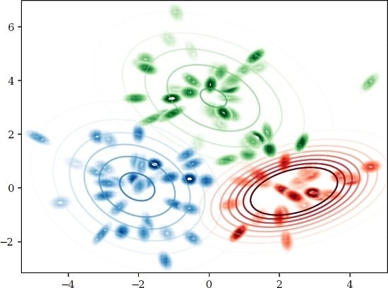
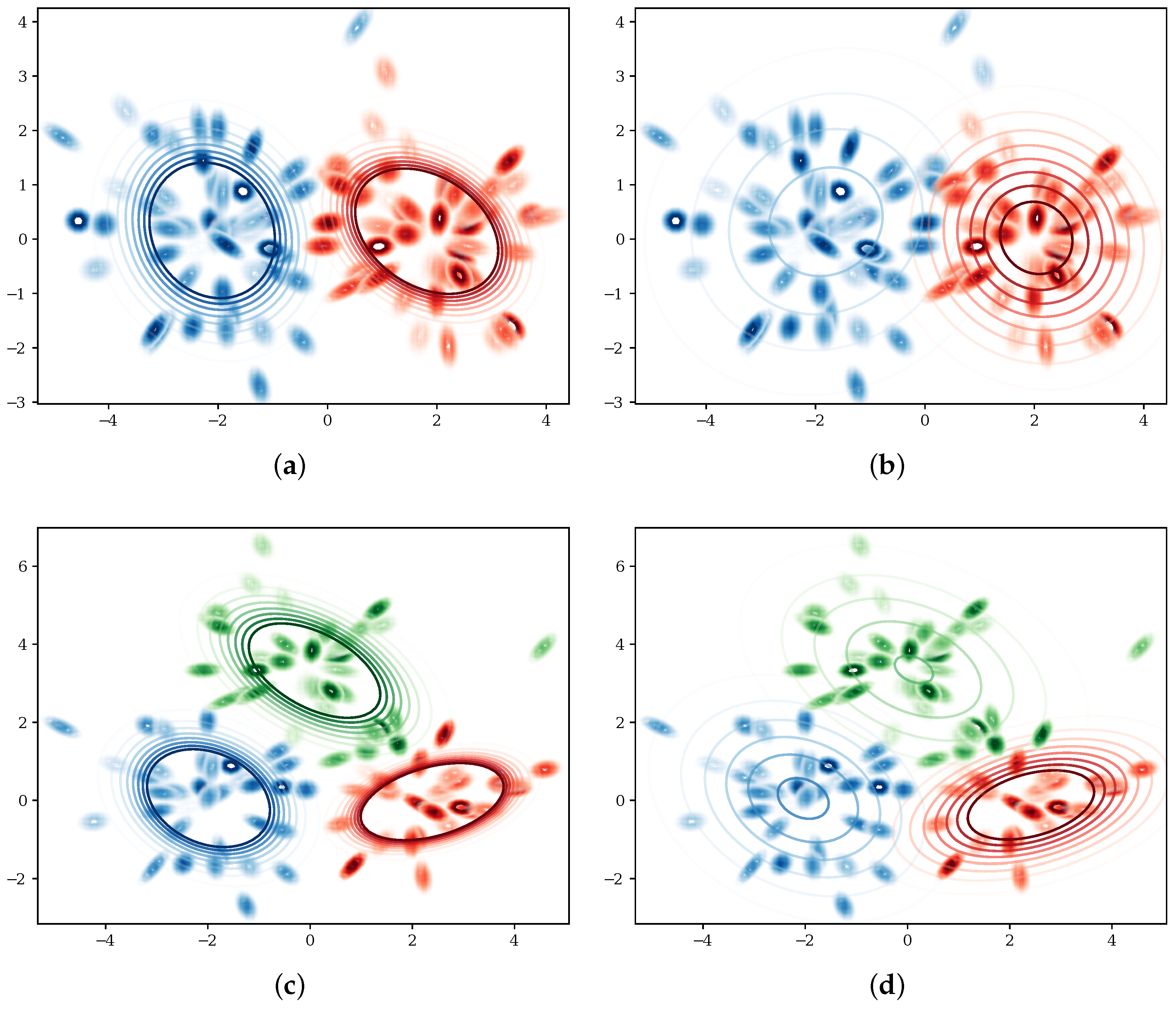
5. Hölder Centroids and Center-Based Clustering

We study the application of HPD and HD for clustering distributions [30], specially clustering Gaussian distributions [31,32,33], which have been used in sound processing [31], sensor network [32], statistical debugging [32], quadratic invariants of switched systems [34], etc. Other potential applications of HD may include nonnegative matrix factorization [35], and clustering von Mises–Fisher [36,37] (log-normalizer expressed using Bessel functions).

5.1. Hölder Centroids

We study center-based clustering of a finite set of distributions belonging to the same exponential family. By a slight abuse of notation, we shall write $D_{\alpha ,\sigma ,\tau }^{\mathtt{H}}(\theta :{\theta }^{\prime })$ instead of $D_{\alpha ,\sigma ,\tau }^{\mathtt{H}}(p_{\theta }:p_{{\theta }^{\prime }})$. Given a list of distributions belonging to the same conic exponential family with natural parameters $\{{\theta }_1,\cdots ,{\theta }_n\}$ and their associated positive weights $\{w_1,\cdots ,w_n\}$ with ${\sum }_{i=1}^n{w}_i=1$, consider their centroids based on HPD and HD as follows:

$$\begin{array}{cc}\hfill C_{\alpha }(\{{\theta }_i,w_i\})& =\underset{C}{\arg \min }{\displaystyle \sum _{i=1}^n}{w}_i{D}_{\alpha ,1,1}^{\mathtt{H}}({\theta }_i:C),\hfill \end{array}$$

(73)

$$\begin{array}{cc}\hfill C_{\alpha ,\gamma }(\{{\theta }_i,w_i\})& =\underset{C}{\arg \min }{\displaystyle \sum _{i=1}^n}{w}_i{D}_{\alpha ,\gamma }^{\mathtt{H}}({\theta }_i:C).\hfill \end{array}$$

(74)

By an abuse of notation, C denotes both the HPD centroid and HD centroid. When the context is clear, the parameters in parentheses can be omitted so that these centroids are simply denoted as $C_{\alpha }$ and $C_{\alpha ,\gamma }$. Both of them are defined as the right-sided centroids. The corresponding left-handed centroids are obtained according to reference duality, i.e.,

$$\begin{array}{cc}\hfill C_{\overline{\alpha }}& =\underset{C}{\arg \min }{\displaystyle \sum _{i=1}^n}{w}_i{D}_{\alpha ,1,1}^{\mathtt{H}}(C:{\theta }_i),\hfill \end{array}$$

(75)

$$\begin{array}{cc}\hfill C_{\overline{\alpha },\gamma }& =\underset{C}{\arg \min }{\displaystyle \sum _{i=1}^n}{w}_i{D}_{\alpha ,\gamma }^{\mathtt{H}}(C:{\theta }_i).\hfill \end{array}$$

(76)

By Lemma 1, these centroids can be obtained for distributions belonging to the same exponential family as follows:

$$\begin{array}{cc}\hfill C_{\alpha }& =\underset{C}{\arg \min }\left[\frac{1}{\beta }F(\beta C)-{\displaystyle \sum _{i=1}^n}{w}_{i}F({\theta }_i+C)\right],\hfill \end{array}$$

(77)

$$\begin{array}{cc}\hfill C_{\alpha ,\gamma }& =\underset{C}{\arg \min }\left[\frac{1}{\beta }F(\gamma C)-{\displaystyle \sum _{i=1}^n}{w}_{i}F\left(\frac{\gamma }{\alpha }{\theta }_i+\frac{\gamma }{\beta }C\right)\right].\hfill \end{array}$$

(78)

Let $\gamma =\alpha$; we get:

$$C_{\alpha ,\alpha }(\{{\theta }_i,w_i\})=\underset{C}{\arg \min }\left[\frac{1}{\beta }F(\alpha C)-{\displaystyle \sum _{i=1}^n}{w}_{i}F\left({\theta }_i+\frac{\alpha }{\beta }C\right)\right]=\frac{\beta }{\alpha }{C}_{\alpha }=\frac{1}{\alpha -1}{C}_{\alpha }(\{{\theta }_i,w_i\}),$$

(79)

meaning that the HPD centroid is just a special case of HD centroid up to a scaling transformation in the natural parameters space. Let $\gamma =\beta$; we get:

$$C_{\alpha ,\beta }(\{{\theta }_i,w_i\})={\arg \min }_C\left[\frac{1}{\beta }F(\beta C)-{\sum }_{i=1}^n{w}_{i}F\left(\frac{\beta }{\alpha }{\theta }_i+C\right)\right]=C_{\alpha }\left(\left\{\frac{\beta }{\alpha }{\theta }_i,w_i\right\}\right)=C_{\alpha }\left(\left\{\frac{1}{\alpha -1}{\theta }_i,w_i\right\}\right).$$

(80)

Let us consider the general HD centroid $C_{\alpha ,\gamma }$. Since F is convex, the minimization energy is the sum of a convex function $\frac{1}{\beta }F(\gamma C)$ with a concave function $-{\sum }_{i=1}^n{w}_{i}F\left(\frac{\gamma }{\alpha }{\theta }_i+\frac{\gamma }{\beta }C\right)$. We can therefore use the concave-convex procedure (CCCP) [8] that optimizes the difference of convex programs (DCPs): We start with $C_{\alpha ,\gamma }^0={\sum }_{i=1}^n{w}_i{\theta }_i$ (the barycenter, belonging to Θ) and then update:

$$C_{\alpha ,\gamma }^{t+1}=\frac{1}{\gamma }{(\nabla F)}^{-1}\left(\sum _{i=1}^n{w}_i\nabla F\left(\frac{\gamma }{\alpha }{\theta }_i+\frac{\gamma }{\beta }{C}_{\alpha ,\gamma }^t\right)\right)$$

(81)

for $t=0,1,\cdots$ until convergence. This can be done by noting that $\eta =\nabla F(\theta )$ are the dual parameters that are also known as the expectation parameters (or moment parameters). Therefore, $\nabla F$ and ${(\nabla F)}^{-1}$ can be computed through Legendre transformations between the natural parameter space and the dual parameter space.

This iterative optimization is guaranteed to converge to a local minimum, with a main advantage of bypassing the learning rate parameter of gradient descent algorithms. Since F is strictly convex, $\nabla F$ is monotonous, and the rhs expression can be interpreted as a multi-dimensional quasi-arithmetic mean. In fact, it is a barycenter on unnormalized weights scaled by $\beta =\overline{\alpha }$.

For exponential families, the symmetric HPD centroid is:

$$O_{\alpha }=\underset{O}{\arg \min }\sum _{i=1}^n{w}_i{S}_{\alpha ,1,1}^{\mathtt{H}}({\theta }_i:O)=\underset{O}{\arg \min }\left[\frac{1}{2\alpha }F(\alpha O)+\frac{1}{2\beta }F(\beta O)-\sum _{i=1}^n{w}_{i}F({\theta }_i+O)\right].$$

(82)

In this case, the CCCP update rule is not in closed form because we cannot easily inverse the sum of gradients (but when $\alpha =\beta$, the two terms collapse, so the CS centroid can be calculated using CCCP). Nevertheless, we can implement the reciprocal operation numerically. Interestingly, the symmetric HD centroid can be solved by CCCP! It amounts to solving:

$$\begin{array}{ccc}\hfill O_{\alpha ,\gamma }& =& \underset{O}{\arg \min }{\displaystyle \sum _{i=1}^n}{w}_i{S}_{\alpha ,\gamma }^{\mathtt{H}}({\theta }_i:O)\hfill \\ & =& \underset{O}{\arg \min }\left[F(\gamma O)-{\displaystyle \sum _{i=1}^n}{w}_i\left(F\left(\frac{\gamma }{\alpha }{\theta }_i+\frac{\gamma }{\beta }O\right)+F\left(\frac{\gamma }{\beta }{\theta }_i+\frac{\gamma }{\alpha }O\right)\right)\right].\hfill \end{array}$$

(83)

One can apply CCCP to iteratively update the centroid based on:

$$O_{\alpha ,\gamma }^{t+1}=\frac{1}{\gamma }{(\nabla F)}^{-1}\left[{\displaystyle \sum _{i=1}^n}{w}_i\left(\frac{1}{\beta }\nabla F\left(\frac{\gamma }{\alpha }{\theta }_i+\frac{\gamma }{\beta }{O}_{\alpha ,\gamma }^t\right)+\frac{1}{\alpha }\nabla F\left(\frac{\gamma }{\beta }{\theta }_i+\frac{\gamma }{\alpha }{O}_{\alpha ,\gamma }^t\right)\right)\right].$$

(84)

Notice the similarity with the updating procedure of $C_{\alpha ,\gamma }^t$.

Once the centroid, say $O_{\alpha ,\gamma }$, has been computed, we calculate the associated Hölder information:

$$\sum _{i=1}^n{w}_i{S}_{\alpha ,\gamma }^{\mathtt{H}}({\theta }_i:O_{\alpha ,\gamma }),$$

(85)

which generalizes the notion of variance and Bregman information [5] to the case of Hölder distances.

5.2. Clustering Based on Symmetric Hölder Divergences

Given a set of fixed densities $\{p_1,\cdots ,p_n\}$, we can perform variational k-means [6] with respect to the Hölder divergence to minimize the cost function:

$$E(O_1,\cdots ,O_L,l_1,\cdots ,l_n)=\sum _{i=1}^n{S}_{\alpha ,\gamma }^{\mathtt{H}}(p_i:O_{l_i}),$$

(86)

where $O_1,\cdots ,O_L$ are the cluster centers and $l_i\in \{1,\cdots ,L\}$ is the cluster label of $p_i$. The algorithm is given by Algorithm 1. Notice that one does not need to wait for the CCCP iterations to converge. It only has to improve the cost function E before updating the assignment. We have implemented the algorithm based on the symmetric HD. One can easily modify it based on HPD and other variants.

Algorithm 1: Hölder variational k-means.

We made a toy dataset generator, which can randomly generate n 2D Gaussians that have an underlying structure of two or three clusters. In the first cluster, the mean of each Gaussian $G(\mu ,\Sigma )$ has the prior distribution $\mu \sim G((-2,0),I)$; the covariance matrix is obtained by first generating ${\sigma }_1\sim \mathrm{\Gamma }(7,0.01)$, ${\sigma }_2\sim \mathrm{\Gamma }(7,0.003)$, where Γ means a gamma distribution with prescribed shape and scale, then rotating the covariance matrix $\mathrm{diag}({\sigma }_1,{\sigma }_2)$ so that the resulting Gaussian has a “radial direction” with respect to the center $(-2,0)$. The second and third clusters are similar to the first cluster with the only difference being that their μ’s are centered around $(2,0)$ and $(0,2\sqrt{3})$, respectively. See Figure 4 for an intuitive presentation of the toy dataset.

To reduce the number of parameters that has to be tuned, we only investigate the case $\alpha =\gamma$. If we choose $\alpha =\gamma =2$, then $S_{\alpha ,\gamma }^{\mathtt{H}}$ becomes the CS divergence, and Algorithm 1 reduces to traditional CS clustering. From Figure 4, we can observe that the clustering result does vary with the settings of α and γ. We performed clustering experiments on two different settings of the number of clusters and two different settings of the sample size.

Table 1. Clustering accuracy of the 2D Gaussian dataset (based on 1000 independent runs). CS, Cauchy–Schwarz. Bold numbers indicate the best obtained performance.

k (#Clusters)	n (#Samples)	$\mathit{\alpha }=\mathit{\gamma }=\mathbf{1.1}$	$\mathit{\alpha }=\mathit{\gamma }=\mathbf{1.5}$	$\mathit{\alpha }=\mathit{\gamma }=\mathbf{2}$ (CS)	$\mathit{\alpha }=\mathit{\gamma }=\mathbf{10}$
2	50	$\mathbf{94.5}\%\pm \mathbf{10.5}\%$	$89.9\%\pm 13.2\%$	$89.4\%\pm 13.5\%$	$88.9\%\pm 14.0\%$
	100	$\mathbf{96.9}\%\pm \mathbf{6.8}\%$	$94.3\%\pm 9.9\%$	$93.8\%\pm 10.6\%$	$93.1\%\pm 11.6\%$
3	50	$\mathbf{84.6}\%\pm \mathbf{15.5}\%$	$79.3\%\pm 14.8\%$	$79.0\%\pm 14.7\%$	$78.7\%\pm 14.5\%$
	100	$\mathbf{89.6}\%\pm \mathbf{13.8}\%$	$83.9\%\pm 14.6\%$	$83.1\%\pm 14.5\%$	$82.8\%\pm 14.4\%$

shows the clustering accuracy measured by the percentage of “correctly-clustered” Gaussians, i.e., the output label by clustering algorithms that coincides with the true label corresponding to the data generating process. The large variance of the clustering accuracy is because different runs are based on different random datasets using the same generator. We see that the symmetric Hölder divergence can give significantly better clustering results as compared to CS clustering. Intuitively, the symmetric Hölder centroid with α and γ close to one has a smaller variance (see Figure 4); therefore, it can better capture the clustering structure. This hints that one should consider the general Hölder divergence to replace CS in similar clustering applications [22,38]. Although one faces the problem of tuning the parameter α and γ, Hölder divergences can potentially give better results. This is expected because CS is just one particular case of the class of Hölder divergences.

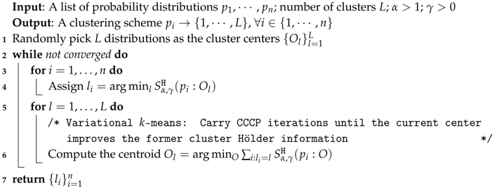
6. Conclusions and Perspectives

We introduced the notion of pseudo-divergences that generalizes the concept of divergences in information geometry [3] that are smooth non-metric statistical distances that are not required to obey the law of the indiscernibles. Pseudo-divergences can be built from inequalities by considering the inequality difference gap or its log-ratio gap. We then defined two classes of statistical measures based on Hölder’s ordinary and reverse inequalities: the tri-parametric family of Hölder pseudo-divergences and the bi-parametric family of Hölder divergences. By construction, the Hölder divergences are proper divergences between probability densities. Both statistical Hölder distance families are projective divergences that do not require distributions to be normalized and admit closed-form expressions when considering exponential families with conic or affine natural parameter space (like multinomials or multivariate normals). Those two families of distances can be symmetrized and encompass both the Cauchy–Schwarz divergence and the family of skew Bhattacharyya divergences. Since the Cauchy–Schwarz divergence is often used in distribution clustering applications [22], we carried out preliminary experiments demonstrating experimentally that the symmetrized Hölder divergences improved over the Cauchy–Schwarz divergence for a toy dataset of Gaussians. We briefly touched upon the use of these novel divergences in statistical estimation theory. These projective Hölder (pseudo-)divergences are different from the recently introduced compositive scored-induced Hölder divergences [17,18] that are not projective divergences and do not admit closed-form expressions for exponential families in general.

We elicited the special role of escort distributions [3] for Hölder divergences in our framework: Escort distributions transform distributions to allow one:

• To reveal that Hölder pseudo-divergences on escort distributions amount to skew Bhattacharyya divergences [8],
• To transform the improper Hölder pseudo-divergences into proper Hölder divergences, and vice versa.

It is interesting to consider other potential applications of Hölder divergences and compare their efficiency against the reference Cauchy–Schwarz divergence: For example, HD t-SNE (Stochastic Neighbor Embedding) compared to CS t-SNE [39], HD vector quantization (VQ) compared to CS VQ [40], HD saliency vs. CS saliency detection in images [41], etc.

Let us conclude with a perspective note on pseudo-divergences, statistical estimators and manifold learning. Proper divergences have been widely used in statistical estimators to build families of estimators [42,43]. Similarly, given a prescribed density $p_0(x)$, a pseudo-divergence yields a corresponding estimator by minimizing $D(p_0:q)$ with respect to $q(x)$. However, in this case, the resulting $q(x)$ is potentially biased and is not guaranteed to recover the optimal input $p_0(x)$. Furthermore, the minimizer of $D(p_0:q)$ may not be unique, i.e., there could be more than one probability density $q(x)$ yielding $D(p_0:q)=0$.

How can pseudo-divergences be useful? We have the following two simple arguments:

• In an estimation scenario, we can usually pre-compute $p_1(x)\ne p_0(x)$ according to $D(p_1:p_0)=0$. Then, the estimation $q(x)=arg{min}_{q}D(p_1:q)$ will automatically target at $p_0(x)$. We call this technique “pre-aim.”
  For example, given positive measure $p(x)$, we first find $p_0(x)$ to satisfy $D_{\alpha ,1,1}^{\mathtt{H}}(p_0:p)=0$. We have $p_0(x)=p{(x)}^{\frac{1}{\alpha -1}}$ that satisfies this condition. Then, a proper divergence between $p(x)$ and $q(x)$ can be obtained by aiming $q(x)$ towards $p_0(x)$. For conjugate exponents α and β,

  $$\begin{array}{cc}\hfill D_{\alpha ,1,1}^{\mathtt{H}}(p_0:q)& =-log\frac{{\int }_{\mathcal{X}}{p}_0(x)q(x)\mathrm{d}x}{{\left({\int }_{\mathcal{X}}{p}_0{(x)}^{\alpha }\mathrm{d}x\right)}^{1/\alpha }{\left({\int }_{\mathcal{X}}q{(x)}^{\beta }\mathrm{d}x\right)}^{1/\beta }}\hfill \\ & =-log\frac{{\int }_{\mathcal{X}}p{(x)}^{\frac{1}{\alpha -1}}q(x)\mathrm{d}x}{{\left({\int }_{\mathcal{X}}p{(x)}^{\frac{\alpha }{\alpha -1}}\mathrm{d}x\right)}^{1/\alpha }{\left({\int }_{\mathcal{X}}q{(x)}^{\beta }\mathrm{d}x\right)}^{1/\beta }}\hfill \\ & =-log\frac{{\int }_{\mathcal{X}}p{(x)}^{\frac{\beta }{\alpha }}q(x)\mathrm{d}x}{{\left({\int }_{\mathcal{X}}p{(x)}^{\beta }\mathrm{d}x\right)}^{1/\alpha }{\left({\int }_{\mathcal{X}}q{(x)}^{\beta }\mathrm{d}x\right)}^{1/\beta }}=D_{\alpha ,\beta }^{\mathtt{H}}(p:q).\hfill \end{array}$$

  (87)
  This means that the pre-aim technique of HPD is equivalent to HD $D_{\alpha ,\gamma }^{\mathtt{H}}$ when we set $\gamma =\beta$.
  As an alternative implementation of pre-aim, since $D_{\alpha ,1,1}^{\mathtt{H}}(p:p^{\alpha -1})=0$, a proper divergence between $p(x)$ and $q(x)$ can be constructed by measuring:

  $$D_{\alpha ,1,1}^{\mathtt{H}}(q:p^{\alpha -1})=-log\frac{{\int }_{\mathcal{X}}p{(x)}^{\frac{\alpha }{\beta }}q(x)\mathrm{d}x}{{\left({\int }_{\mathcal{X}}q{(x)}^{\alpha }\mathrm{d}x\right)}^{1/\alpha }{\left({\int }_{\mathcal{X}}p{(x)}^{\alpha }\mathrm{d}x\right)}^{1/\beta }}=D_{\beta ,\alpha }^{\mathtt{H}}(p:q),$$

  (88)

  turning out again to belong to the class of HD.
  In practice, HD as a bi-parametric family may be less used than HPD with pre-aim because of the difficulty in choosing the parameter γ and because that HD has a slightly more complicated expression. The family of HD connecting CS divergence with skew Bhattacharyya divergence [8] is nevertheless of theoretical importance.
• In manifold learning [44,45,46,47], it is an essential topic to align two category distributions $p_0(x)$ and $q(x)$ corresponding respectively to the input and output [47], both for learning and for performance evaluation. In this case, the dimensionality of the statistical manifold that encompasses $p_0(x)$ and $q(x)$ is so high that to preserve monotonically $p_0(x)$ in the resulting $q(x)$ is already a difficult non-linear optimization and could be sufficient for the application, while preserving perfectly the input $p_0(x)$ is not so meaningful because of the input noise. It is then much easier to define pseudo-divergences using inequalities which do not necessarily need to be proper with potentially more choices. On the other hand, projective divergences including Hölder divergences introduced in this work are more meaningful in manifold learning than KL divergence (which is widely used) because they give scale invariance of the probability densities, meaning that one can define positive similarities then directly align these similarities, which is guaranteed to be equivalent to aligning the corresponding distributions. This could potentially give unified perspectives in between the two approaches of similarity-based manifold learning [46] and the probabilistic approach [44].

Hölder-type inequalities have been generalized to sets [48] instead of pairs of objects and to positive functional spaces, as well [49]. We also note that some divergences like Csiszár f -divergences enjoy themselves Hölder-type inequalities [50].

We expect that these two novel parametric Hölder classes of statistical divergences and pseudo-divergences open up new insights and applications in statistics and information sciences. Furthermore, the framework to build divergences or pseudo-divergences from proper or improper biparametric inequalities [1] offers novel classes of divergences to study.

Reproducible source code is available online [51].

References

1. Mitrinovic, D.S.; Pecaric, J.; Fink, A.M. Classical and New Inequalities in Analysis; Springer Science & Business Media: New York, NY, USA, 2013; Volume 61. [Google Scholar]
2. Budka, M.; Gabrys, B.; Musial, K. On accuracy of PDF divergence estimators and their applicability to representative data sampling. Entropy 2011, 13, 1229–1266. [Google Scholar] [CrossRef]
3. Amari, S.I. Information Geometry and Its Applications; Applied Mathematical Sciences series; Springer: Tokyo, Japan, 2016. [Google Scholar]
4. Rao, C.R. Information and accuracy attainable in the estimation of statistical parameters. Bull. Calcutta Math. Soc. 1945, 37, 81–91. [Google Scholar]
5. Banerjee, A.; Merugu, S.; Dhillon, I.S.; Ghosh, J. Clustering with Bregman divergences. J. Mach. Learn. Res. 2005, 6, 1705–1749. [Google Scholar]
6. Nielsen, F.; Nock, R. Total Jensen divergences: Definition, properties and clustering. In Proceedings of the 2015 IEEE International Conference on Acoustics, Speech and Signal Processing (ICASSP), South Brisbane, Australia, 19–24 April 2015; pp. 2016–2020.
7. Burbea, J.; Rao, C. On the convexity of some divergence measures based on entropy functions. IEEE Trans. Inf. Theory 1982, 28, 489–495. [Google Scholar] [CrossRef]
8. Nielsen, F.; Boltz, S. The Burbea-Rao and Bhattacharyya centroids. IEEE Trans. Inf. Theory 2011, 57, 5455–5466. [Google Scholar] [CrossRef]
9. Gneiting, T.; Raftery, A.E. Strictly proper scoring rules, prediction, and estimation. J. Am. Stat. Assoc. 2007, 102, 359–378. [Google Scholar] [CrossRef]
10. Cover, T.M.; Thomas, J.A. Elements of Information Theory; John Wiley & Sons: Hoboken, NJ, USA, 2012. [Google Scholar]
11. Fujisawa, H.; Eguchi, S. Robust parameter estimation with a small bias against heavy contamination. J. Multivar. Anal. 2008, 99, 2053–2081. [Google Scholar] [CrossRef]
12. Nielsen, F.; Nock, R. Patch Matching with Polynomial Exponential Families and Projective Divergences. In Proceedings of the 9th International Conference on Similarity Search and Applications, Tokyo, Japan, 24–26 October 2016; pp. 109–116.
13. Zhang, J. Divergence function, duality, and convex analysis. Neural Comput. 2004, 16, 159–195. [Google Scholar] [CrossRef] [PubMed]
14. Zhang, J. Nonparametric information geometry: From divergence function to referential-representational biduality on statistical manifolds. Entropy 2013, 15, 5384–5418. [Google Scholar] [CrossRef]
15. Nielsen, F.; Nock, R. A closed-form expression for the Sharma–Mittal entropy of exponential families. J. Phys. A Math. Theor. 2011, 45, 032003. [Google Scholar] [CrossRef]
16. De Souza, D.C.; Vigelis, R.F.; Cavalcante, C.C. Geometry Induced by a Generalization of Rényi Divergence. Entropy 2016, 18, 407. [Google Scholar] [CrossRef]
17. Kanamori, T.; Fujisawa, H. Affine invariant divergences associated with proper composite scoring rules and their applications. Bernoulli 2014, 20, 2278–2304. [Google Scholar] [CrossRef]
18. Kanamori, T. Scale-invariant divergences for density functions. Entropy 2014, 16, 2611–2628. [Google Scholar] [CrossRef]
19. Nielsen, F.; Garcia, V. Statistical exponential families: A digest with flash cards. arXiv, 2009; arXiv:0911.4863. [Google Scholar]
20. Rogers, L.J. An extension of a certain theorem in inequalities. Messenger Math. 1888, 17, 145–150. [Google Scholar]
21. Holder, O.L. Über einen Mittelwertssatz. Nachr. Akad. Wiss. Gottingen Math. Phys. Kl. 1889, 44, 38–47. [Google Scholar]
22. Hasanbelliu, E.; Giraldo, L.S.; Principe, J.C. Information theoretic shape matching. IEEE Trans. Pattern Anal. Mach. Intell. 2014, 36, 2436–2451. [Google Scholar] [CrossRef] [PubMed]
23. Nielsen, F. Closed-form information-theoretic divergences for statistical mixtures. In Proceedings of the 21st International Conference on Pattern Recognition (ICPR), Tsukuba, Japan, 11–15 November 2012; pp. 1723–1726.
24. Zhang, J. Reference duality and representation duality in information geometry. Am. Inst. Phys. Conf. Ser. 2015, 1641, 130–146. [Google Scholar]
25. Bhattacharyya, A. On a measure of divergence between two statistical populations defined by their probability distributions. Bull. Calcutta Math. Soc. 1943, 35, 99–109. [Google Scholar]
26. Srivastava, A.; Jermyn, I.; Joshi, S. Riemannian analysis of probability density functions with applications in vision. In Proceedings of the 2007 IEEE Conference on Computer Vision and Pattern Recognition, Minneapolis, MN, USA, 17–22 June 2007; pp. 1–8.
27. Nielsen, F.; Nock, R. On the Chi Square and Higher-Order Chi Distances for Approximating f-Divergences. IEEE Signal Process. Lett. 2014, 1, 10–13. [Google Scholar] [CrossRef]
28. Nielsen, F.; Nock, R. Skew Jensen-Bregman Voronoi diagrams. In Transactions on Computational Science XIV; Springer: New York, NY, USA, 2011; pp. 102–128. [Google Scholar]
29. Nielsen, F.; Sun, K. Guaranteed Bounds on Information-Theoretic Measures of Univariate Mixtures Using Piecewise Log-Sum-Exp Inequalities. Entropy 2016, 18, 442. [Google Scholar] [CrossRef]
30. Notsu, A.; Komori, O.; Eguchi, S. Spontaneous clustering via minimum gamma-divergence. Neural Comput. 2014, 26, 421–448. [Google Scholar] [CrossRef] [PubMed]
31. Rigazio, L.; Tsakam, B.; Junqua, J.C. An optimal Bhattacharyya centroid algorithm for Gaussian clustering with applications in automatic speech recognition. In Proceedings of the 2000 IEEE International Conference on Acoustics, Speech, and Signal Processing, Istanbul, Turkey, 5–9 June 2000; Volume 3, pp. 1599–1602.
32. Davis, J.V.; Dhillon, I.S. Differential Entropic Clustering of Multivariate Gaussians. In Proceedings of the Advances in Neural Information Processing Systems, Vancouver, BC, Canada, 7–10 December 2006; pp. 337–344.
33. Nielsen, F.; Nock, R. Clustering multivariate normal distributions. In Emerging Trends in Visual Computing; Springer: New York, NY, USA, 2009; pp. 164–174. [Google Scholar]
34. Allamigeon, X.; Gaubert, S.; Goubault, E.; Putot, S.; Stott, N. A scalable algebraic method to infer quadratic invariants of switched systems. In Proceedings of the 12th International Conference on Embedded Software, Amsterdam, The Netherlands, 4–9 October 2015; pp. 75–84.
35. Sun, D.L.; Févotte, C. Alternating direction method of multipliers for non-negative matrix factorization with the beta-divergence. In Proceedings of the 2014 IEEE International Conference on Acoustics, Speech and Signal Processing (ICASSP), Florence, Italy, 4–9 May 2014; pp. 6201–6205.
36. Banerjee, A.; Dhillon, I.S.; Ghosh, J.; Sra, S. Clustering on the unit hypersphere using von Mises-Fisher distributions. J. Mach. Learn. Res. 2005, 6, 1345–1382. [Google Scholar]
37. Gopal, S.; Yang, Y. Von Mises-Fisher Clustering Models. J. Mach. Learn. Res. 2014, 32, 154–162. [Google Scholar]
38. Rami, H.; Belmerhnia, L.; Drissi El Maliani, A.; El Hassouni, M. Texture Retrieval Using Mixtures of Generalized Gaussian Distribution and Cauchy-Schwarz Divergence in Wavelet Domain. Image Commun. 2016, 42, 45–58. [Google Scholar] [CrossRef]
39. Bunte, K.; Haase, S.; Biehl, M.; Villmann, T. Stochastic neighbor embedding (SNE) for dimension reduction and visualization using arbitrary divergences. Neurocomputing 2012, 90, 23–45. [Google Scholar] [CrossRef]
40. Villmann, T.; Haase, S. Divergence-based vector quantization. Neural Comput. 2011, 23, 1343–1392. [Google Scholar] [CrossRef] [PubMed]
41. Huang, J.B.; Ahuja, N. Saliency detection via divergence analysis: A unified perspective. In Proceedings of the 2012 21st International Conference on Pattern Recognition (ICPR), Tsukuba, Japan, 11–15 November 2012; pp. 2748–2751.
42. Pardo, L. Statistical Inference Based on Divergence Measures; CRC Press: Abingdon, UK, 2005. [Google Scholar]
43. Basu, A.; Shioya, H.; Park, C. Statistical Inference: The Minimum Distance Approach; CRC Press: Abingdon, UK, 2011. [Google Scholar]
44. Hinton, G.E.; Roweis, S.T. Stochastic Neighbor Embedding. In Advances in Neural Information Processing Systems 15 (NIPS); MIT Press: Vancouver, BC, Canada, 2002; pp. 833–840. [Google Scholar]
45. Maaten, L.V.D.; Hinton, G. Visualizing data using t-SNE. J. Mach. Learn. Res. 2008, 9, 2579–2605. [Google Scholar]
46. Carreira-Perpiñán, M.Á. The Elastic Embedding Algorithm for Dimensionality Reduction. In Proceedings of the International Conference on Machine Learning, Haifa, Israel, 21–25 June 2010; pp. 167–174.
47. Sun, K.; Marchand-Maillet, S. An Information Geometry of Statistical Manifold Learning. In Proceedings of the International Conference on Machine Learning, Beijing, China, 21–26 June 2014; pp. 1–9.
48. Cheung, W.S. Generalizations of Hölder’s inequality. Int. J. Math. Math. Sci. 2001, 26, 7–10. [Google Scholar] [CrossRef]
49. Hazewinkel, M. Encyclopedia of Mathematics; Kluwer Academic Publishers: Dordrecht, The Netherlands, 2001. [Google Scholar]
50. Chen, G.S.; Shi, X.J. Generalizations of Hölder inequalities for Csiszár’s f -divergence. J. Inequal. Appl. 2013, 2013, 151. [Google Scholar] [CrossRef]
51. Nielsen, F.; Sun, K.; Marchand-Maillet, S. On Hölder Projective Divergences. 2017. Available online: https://www.lix.polytechnique.fr/~nielsen/HPD/ (accessed on 16 March 2017).
52. Boyd, S.; Vandenberghe, L. Convex Optimization; Cambridge University Press: Cambridge, UK, 2004. [Google Scholar]
Figure 1. Hölder proper divergence (bi-parametric) and Hölder improper pseudo-divergence (tri-parametric) encompass Cauchy–Schwarz divergence and skew Bhattacharyya divergence.
Entropy 19 00122 g001
Figure 2. First row: the Hölder pseudo divergence (HPD) D α , 1 , 1 H ( p r : p ) for α { 4 / 3 , 2 , 4 } , KL divergence and reverse KL divergence. Remaining rows: the HD D α , γ H ( p r : p ) for α { 4 / 3 , 1.5 , 2 , 4 , 10 } (from top to bottom) and γ { 0.5 , 1 , 2 , 5 , 10 } (from left to right). The reference distribution p r is presented as “★”. The minimizer of D α , 1 , 1 H ( p r : p ) , if different from p r , is presented as “•”. Notice that D 2 , 2 H = D 2 , 1 , 1 H . (a) Reference categorical distribution p r = ( 1 / 3 , 1 / 3 , 1 / 3 ) ; (b) reference categorical distribution p r = ( 1 / 2 , 1 / 3 , 1 / 6 ) .
Entropy 19 00122 g002aEntropy 19 00122 g002b
Figure 3. First row: D α , 1 , 1 H ( p r : p ) , where p r is the standard Gaussian distribution and α { 4 / 3 , 2 , 4 } compared to the KL divergence. The rest of the rows: D α , γ H ( p r : p ) for α { 4 / 3 , 1.5 , 2 , 4 , 10 } (from top to bottom) and γ { 0.5 , 1 , 2 , 5 , 10 } (from left to right). Notice that D 2 , 2 H = D 2 , 1 , 1 H . The coordinate system is formed by μ (mean) and σ (standard deviation).
Entropy 19 00122 g003
Figure 4. Variational k-means clustering results on a toy dataset consisting of a set of 2D Gaussians organized into two or three clusters. The cluster centroids are represented by contour plots using the same density levels. (a) α = γ = 1.1 (Hölder clustering); (b) α = γ = 2 (Cauchy–Schwarz clustering); (c) α = γ = 1.1 (Hölder clustering); (d) α = γ = 2 (Cauchy–Schwarz clustering).
Entropy 19 00122 g004