Article

Permutation Entropy: Too Complex a Measure for EEG Time Series?

1
Department of Anaesthesiology, Klinikum rechts der Isar der Technischen Universität München (MRI TUM), 81675 Munich, Germany
2
Institute of Geomatics Engineering, University of Applied Sciences and Arts Northwestern Switzerland, 4132 Muttenz, Switzerland
*
Author to whom correspondence should be addressed.
Entropy 2017, 19(12), 692; https://doi.org/10.3390/e19120692
Submission received: 16 November 2017 / Revised: 11 December 2017 / Accepted: 13 December 2017 / Published: 16 December 2017
(This article belongs to the Special Issue Permutation Entropy & Its Interdisciplinary Applications)

Abstract

:
Permutation entropy (PeEn) is a complexity measure that originated from dynamical systems theory. Specifically engineered to be robustly applicable to real-world data, the quantity has since been utilised for a multitude of time series analysis tasks. In electroencephalogram (EEG) analysis, value changes of PeEn correlate with clinical observations, among them the onset of epileptic seizures or the loss of consciousness induced by anaesthetic agents. Regarding this field of application, the present work suggests a relation between PeEn-based complexity estimation and spectral methods of EEG analysis: for ordinal patterns of three consecutive samples, the PeEn of an epoch of EEG appears to approximate the centroid of its weighted power spectrum. To substantiate this proposition, a systematic approach based on redundancy reduction is introduced and applied to sleep and epileptic seizure EEG. The interrelation demonstrated may aid the interpretation of PeEn in EEG, and may increase its comparability with other techniques of EEG analysis.

1. Introduction

Electroencephalography (EEG) is a neurophysiological technique widely used in research and medical diagnostics. Regardless of its broad spectrum of applications, a common denominator of working with EEG is the assessment of motifs/patterns/features in the signals, and to relate them to observations from other modalities. Analyses are either performed by visual inspection or supported by computer-based parameter extraction. Ultimately, the purpose of EEG analysis is the inference on cortical state changes.
EEG signals are varying electrical potentials that are (in most cases) non-invasively measured across the scalp. These voltage fluctuations represent a very low-dimensional projection of the underlying cerebral processes, and their relation to higher cortical functions is not fully understood. Most techniques of quantitative EEG analysis are therefore intrinsically empirical. Be it the classic frequency band-related measures or more recent additions to the set of analysis tools: the mechanistic background of the vast majority of EEG parameters is not entirely known. In this inherently probabilistic framework, any given signal property that correlates with behavioural observations constitutes a parameter worth considering for EEG analysis.
One quantity that is receiving increasing attention in the field is permutation entropy (PeEn). Introduced by Christoph Bandt and Bernd Pompe as a complexity measure for time series, PeEn is the Shannon entropy of a sequence of ordinal patterns—the latter being discrete symbols that encode how consecutive time series entries relate to one another in terms of position and value [1]. PeEn has been successfully used for EEG analyses in sleep scoring, general anaesthesia monitoring and research on disorders of the central nervous system, most notably epilepsy. Comprehensive overviews regarding the manifold applications of PeEn can be found in [2,3].
New applications of PeEn in EEG processing, and especially ways of extending the method are constantly reported on. For instance, “weighted” [4], “multiscale” [5], “multivariate multi-scale” [6], and “amplitude-aware” [7] variants of PeEn have so far been proposed. As literature suggests, the quantity may well be relevant to any research field that benefits from a widely accepted measure of the complexity of EEG.
Considering the great interest taken in PeEn, and given its virtually universal applicability in EEG analysis, a particular set of questions is surprisingly seldom addressed: what are the dynamic signal characteristics of EEG that PeEn responds to? Can the parameters pattern order and time delay be selected on a phenomenological basis? How should the abstract notion of complexity be interpreted in EEG?
From the outcome-oriented perspective, these may be minor issues. Nevertheless, a careful examination of PeEn in EEG might foster our general understanding of this class of electrophysiological signals. The present work takes a step in this direction, pioneering the following approach: (1) instead of extending PeEn, try to simplify it without compromising its suitability for EEG analysis; and (2) if successful, examine whether the result can more easily be interpreted than the initial chaos-theoretic complexity measure.
Credit for inspiring this idea is due to Bandt [8], who recently questioned the usage of terms like “complexity”, “chaos” and “disorder” in the EEG context and suggested that the PeEn of an epoch of EEG is equivalent to its distance from white noise—a simplification that immediately increases interpretability. In the following article, we shall advance this strategy, systematically deriving an intuitive explanation for the behaviour of PeEn in EEG.

2. An Overview of Permutation Entropy

Both the terminology and mathematical formulation regarding PeEn may vary between authors. To avoid ambiguity, it seems reasonable to shortly recapitulate the basic principles underlying the quantity—using the definitions, notations and nomenclature this work will adhere to.

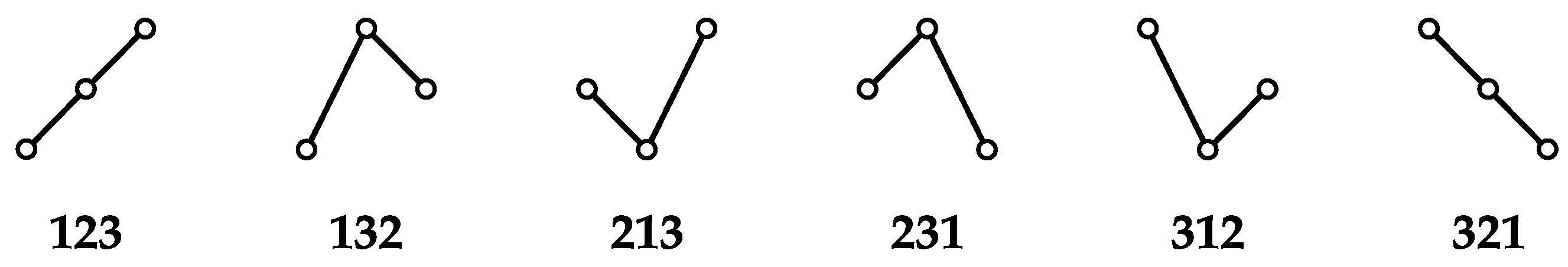
2.1. Sequences of Ordinal Patterns

The ordinal pattern of an m-tuple of real numbers ( x 1 , x 2 , , x m ) describes how its elements relate to one another in terms of position and value. For instance, the ordinal pattern of the tuple ( 17 , 7 , 8 ) is fully specified by: “There are three elements, the first is the greatest, the second is the least.”
Apart from didactic purposes, formal representations of ordinal patterns are usually preferred. Let us hereto agree upon the following simple notation: each element x i of an m-tuple ( x 1 , x 2 , , x m ) shall be assigned a distinct index k i { 1 , 2 , , m } , whereby the greatest element is assigned the index m, the second-greatest is assigned the index m 1 , and so forth. The ordinal pattern of the aforementioned tuple ( 17 , 7 , 8 ) thus corresponds to the indices ( k 1 , k 2 , k 3 ) = ( 3 , 1 , 2 ) . We shall simply write  312 when referring to this specific pattern.
Only tuples of pairwise distinct elements can have an unambiguous ordinal pattern. Let us neglect this latent ambiguity, limiting our considerations to tuples ( x 1 , x 2 , , x m ) with x i = x j if and only if i = j . For any such tuple, each permutation of its set of values { x i } results in a different ordinal pattern. Consequently, a set of m ! ordinal patterns Ω m = { Π 1 , Π 2 , , Π m ! } exists for tuples of length m. The parameter m 2 is called the order of the ordinal pattern.
Consider, for example, the tuple ( x 1 , x 2 , x 3 ) with x 1 x 2 x 3 . Its m ! = 6 possible ordinal patterns of order m = 3 shall be denoted Ω 3 = { 123 , 132 , 213 , 231 , 312 , 321 } . Figure 1 displays the shapes of these ordinal patterns.
Any sequence of real numbers ( x 1 , x 2 , , x n ) can be mapped onto a sequence of ordinal patterns. Given the order m, the particular pattern π t at time index t is obtained from the m-tuple of values
( x t , x t + τ , x t + 2 τ , , x t + ( m 1 ) τ ) π t Ω m .
This encoding is frequently called the symbolisation technique and yields an ordinal pattern sequence of the form
( π 1 , π 2 , , π k ) with k = n ( m 1 ) τ ,
where k is the number of patterns obtainable from a sequence of n samples. The parameter τ 1 represents the distance between samples compared and is usually named the time delay.

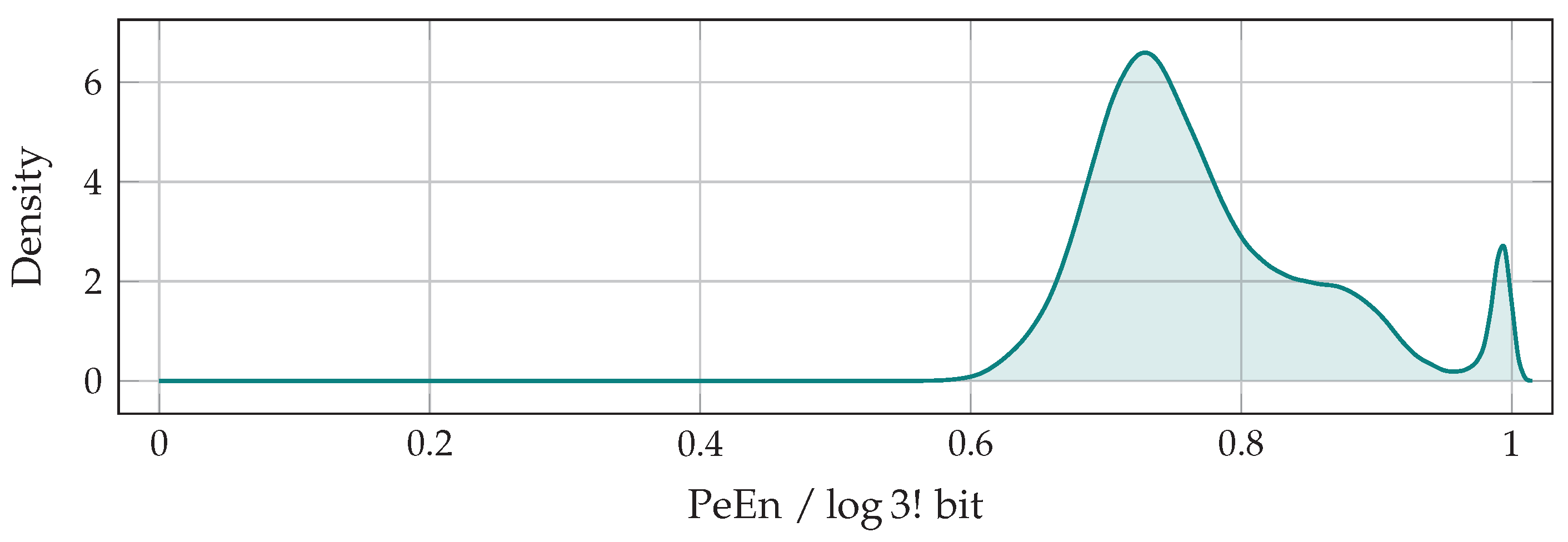
2.2. Estimating the Permutation Entropy of EEG

PeEn of order m and time delay τ is the Shannon entropy [9] of a discrete probability distribution of m !  ordinal patterns. In EEG analysis, the probability distribution vector
p = p 1 p 2 p m ! T and p 1 = 1
is obtained by first mapping a sequence of EEG samples ( x 1 , x 2 , , x n ) onto its corresponding sequence of ordinal patterns ( π 1 , π 2 , , π k ) in terms of Equations (1) and (2). The probability distribution p is then estimated by counting pattern occurrences. For a sequence of k elements, the probability p i of the pattern Π i Ω m is hence
p i = 1 k t = 1 k π t = Π i for 1 i m ! = | Ω m | .
The operator · represents the Iverson bracket [10], a convenient means of notating anonymous indicator functions. Shannon entropy is then computed from the probability distribution p according to the fundamental formula
H ( p ) = i = 1 m ! p i log 1 p i .
For any p i = 0 , the corresponding summand is replaced by the value of its limit towards zero,
lim p i 0 p i log 1 p i = 0 .
PeEn thus converges for any given ordinal pattern distribution. The base of the logarithm can be chosen arbitrarily and determines the unit of measure. Entropy values reported in this work were divided by log m ! for normalisation—they are dimensionless quantities on the interval  [ 0 , 1 ] .

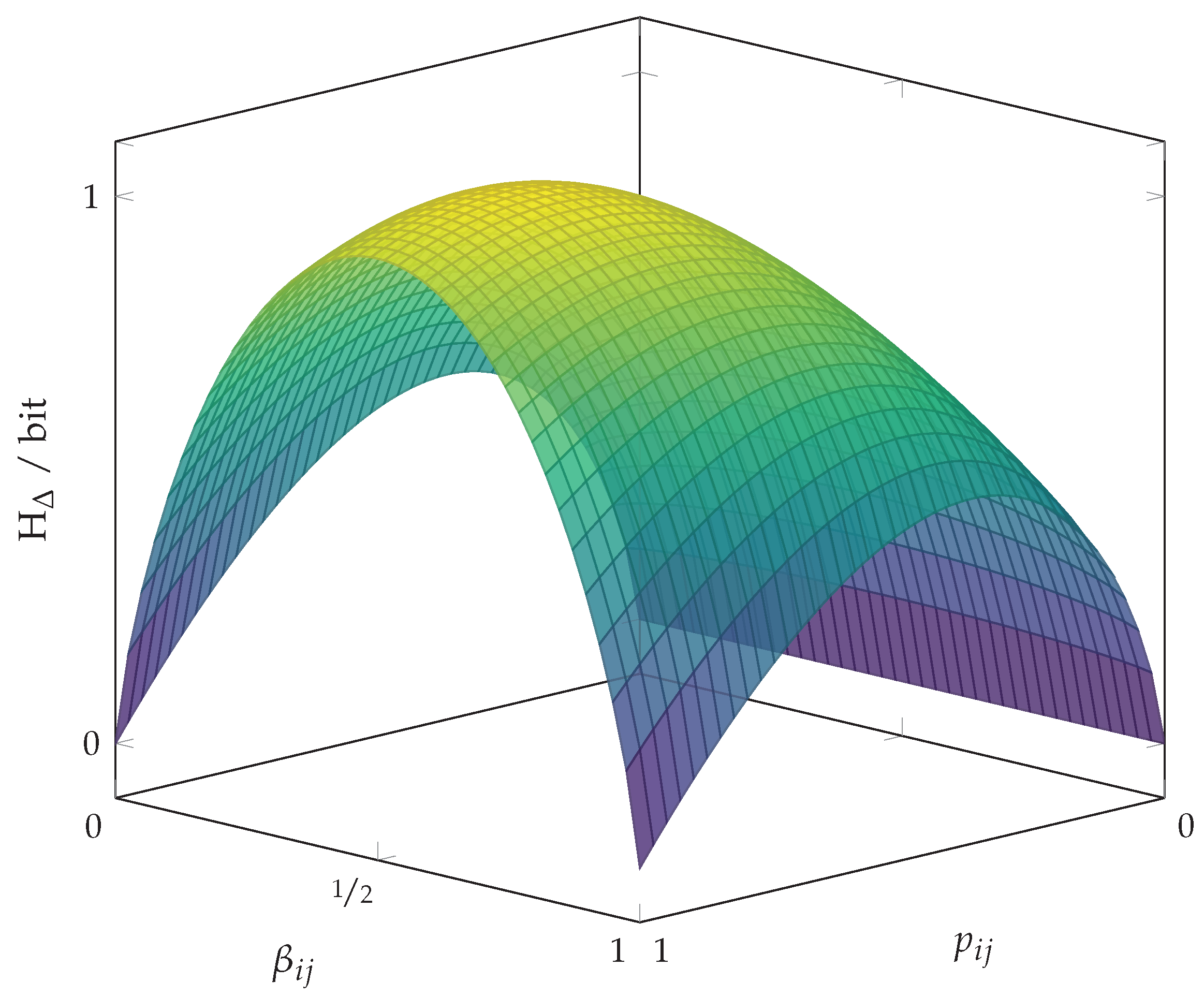
3. Shannon Entropy and Pairwise Probability Balances

No matter the unit of measure: the absolute value of PeEn as obtained from a single epoch of EEG is insignificant. Conversely, the quantity is highly relevant for EEG analysis when comparing entropies across multiple EEG epochs. Considerable contrast in value can then be observed (and be correlated with behavioural observations as is common practice). Let us call these decisive inter-epoch fluctuations the dynamics of PeEn. Their relation with the signal characteristics of EEG are the main topic of the article at hand. To approach the subject, we shall consider some properties of Shannon entropy and derive implications for the dynamics of PeEn therefrom.

Pairwise Probability Balances

From a model-free perspective, Shannon entropy can be interpreted as a statistical parameter on a discrete probability distribution
p = p 1 p 2 p n T and p 1 = 1 .
One of its core properties is that it increases with any pairwise modification of p towards the uniform distribution [9]. To utilise this behaviour, let us partition the n elements of p into a set of n 2 probability pairs
X = ( p i , p j ) ( i , j ) 1 , , n × 1 , , n ,
and let us further define for each such pair ( p i , p j ) a probability balance coefficient
β i j = p i / ( p i + p j ) for p i + p j > 0 , 1 / 2 for p i + p j = 0 .
It then holds that β i j = 1 / 2 if and only if p i = p j . In analogy to the steady continuation of Shannon entropy as per Equation (6), this justifies the stipulation β i j = 1 / 2 for p i + p j = 0 . Moreover, it holds that
β i j + β j i = 1 .
Using its balance coefficient β i j , the contribution of a particular probability p i to the overall value of Shannon entropy can be expressed as
p i log 1 p i = p i log 1 p i + p j + p i log p i + p j p i = p i log 1 p i + p j + p i log 1 β i j .
The summed contribution of a probability pair ( p i , p j ) then is
p i log 1 p i + p j log 1 p j = p i log 1 p i + p j + p i log 1 β i j + p j log 1 p i + p j + p j log 1 β j i = ( p i + p j ) log 1 p i + p j + β i j log 1 β i j + ( 1 β i j ) log 1 1 β i j = ( p i + p j ) log 1 p i + p j + H b ( β i j ) .
The right-hand side of this equation is an affine transformation of the binary entropy function
H b ( x ) = x log 1 x + ( 1 x ) log 1 1 x .
Introducing p i j = p i + p j , Equation (12) can be reformulated as the bivariate function
H Δ ( p i j , β i j ) = p i j log 1 p i j + p i j H b ( β i j ) ,
which behaves as depicted in Figure 2. In particular, if we fix the summed probability p i j at a constant value, H Δ is a concave function on the domain 0 β i j 1 . This function is symmetrical with regard to its maximum at β i j = 1 / 2 , where p i = p j . Thus, if we reallocate among a pair ( p i , p j ) their summed probability p i j such that p i and p j approach their average (while p i j remains constant), β i j approaches  1 / 2 and Shannon entropy increases. The same principle applies to any pair of probabilities drifting apart, where the entropy decreases. Two well-known corner cases of this generic property are that (1) Shannon entropy is maximal for the uniform distribution, while (2) it is zero if all but one p i are zero [9].
For a probability distribution p of n elements, a quadratic matrix of n 2 balance coefficients
β 11 β 1 n β n 1 β n n
can be created. We limit our considerations to the entries above its main diagonal, namely the subset
B = β i j | 1 i < j n such that | B | = n 2 = n 2 + n 2 .
The remaining coefficients, β i j with i j , are easily obtained via the property of symmetry as given by Equation (10).
In conjunction with the relation p 1 = 1 , the coefficients β i j B constitute a system of | B | + 1 linear equations in the probabilities  p . Its augmented system matrix is
1 1 1 1 1 1 β 12 1 β 12 0 0 0 0 β 13 1 0 β 13 0 0 0 β 14 1 0 0 β 14 0 0 0 0 0 0 β n 1 , n 0 .
By Gaussian elimination, one confirms this system to be overdetermined but consistent. Any probability distribution vector p is hence unambiguously determined by its corresponding set of balance coefficients β i j B . The same holds true for the value of Shannon entropy H ( p ) . Consequently, the dynamics of PeEn can be studied by analysing variations within the probability balances β i j B .

4. Complexity and Pseudo-Complexity

PeEn depends on a set of parameters and surrounding conditions. Besides the order m and time delay  τ , also the sampling rate  f s , the window length n as well as any filters applied to the EEG may affect the results. Those are a lot of parameters to decide upon, especially when considering the empirical nature of ordinal pattern-based EEG analysis. Existing guidelines on parameter selection are essentially based on computational or statistical feasibility concerns [3], and are rather not motivated by (electro-)physiological considerations. Therefore, any parametrisation of PeEn reported suitable for EEG analysis must be regarded as the result of extensive experimentation.
With that in mind, it is remarkable that independent groups have successfully used the six ordinal patterns of order m = 3 for EEG encoding [11]. Most likely by experimental optimisation, investigators ended up using the lowest-possible order that still accounts for more than just the patterns “the signal increases”  ( 12 ) versus “the signal decreases”  ( 21 ) . Paradoxically, if six ordinal patterns suffice for the analysis, most of what makes PeEn a complexity measure can apparently be omitted.
Accepting this immanent contradiction, one may raise the following questions: can the number of ordinal patterns be even further reduced without impairing the dynamics of PeEn? If so, do the remaining patterns permit a more tangible interpretation of this EEG analysis technique?

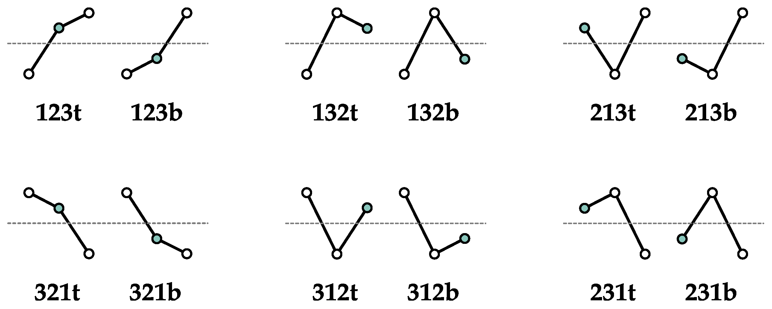
4.1. A New Class of Ordinal Patterns?

Regarding these questions, variegating the pattern order m obviously does not permit any further investigation. A finer-grained approach is necessary and shall here be introduced. It is based on the idea that any pattern pair may be the redundant bifurcation of a less specialised, yet more decisive kind of motif.
By way of illustration, let us define an augmented class of ordinal patterns of order m = 3 . For any tuple of distinct values ( x 1 , x 2 , x 3 ) , our extra-ordinal patterns shall not only describe how its elements relate to one another, but additionally encode the value of the Boolean expression
( x hi x mid ) ( x mid x lo ) .
Figuratively, we assess if the centroid of a pattern lies above or below its equatorial axis. This is visualised in Figure 3.
Consequently, we shall call the respective pattern either top-heavy or bottom-heavy. As an example, the tuple ( 23 , 11 , 14 ) features the bottom-heavy pattern 312 b , while the tuple ( 28 , 6 , 17 ) maps onto a top-heavy 312 t . Both patterns are derivates of the same (conventional) ordinal pattern 312 , though, and it holds for their probabilities that p 312 = p 312 t + p 312 b . Generally, a pair of extra-ordinal patterns  Π t i  and  Π b i exists for each ordinal pattern Π i , and their probabilities relate to each other as in
p i = p t i + p b i .
In practice, calculating this extra-ordinary permutation entropy (XPeEn) only marginally differs from the standard approach: probability distribution estimates for 2 × m ! = 12 distinct patterns are to be obtained.

4.2. Pseudo-Complexity in Ordinal Pattern Analysis

Apart from nomenclature, XPeEn is theoretically a reasonable extension. Using conventional PeEn of order m = 3 , we implicitly agree to distinguish two upward-peak patterns ( 132 and 231 ) as well as two downward-peak patterns ( 213 and 312 ). By implication, the additional distinction between top-heavy and bottom-heavy patterns is then equally justified. Both kinds of partitions stem from the same principle, and the degree of granularity that better matches the signal characteristics of EEG is not evident: ultimately, the relations between ordinal patterns and EEG are not understood.
Understood are, however, the properties of Shannon entropy. According to Equation (14), and in conjunction with Equation (19), it holds for any pair of extra-ordinal patterns Π t i  and  Π b i that their summed contribution to XPeEn is
H Δ ( p i , β i ) = p t i log 1 p t i + p b i log 1 p b i = p i H b ( β i ) + p i log 1 p i ,
where β i is the probability balance coefficient
β i = p t i p t i + p b i = p t i p i .
By estimating the variance of a particular β i from a suitably large collection of EEG epochs, we can thus quantify the impact its corresponding pattern pair Π t i  and  Π b i has on the dynamics of XPeEn. As an example as intuitive as unlikely, imagine that the variance of some balance coefficient β i is found to be zero, such that β i and H b ( β i ) remain constant for any epoch of EEG. Equation (20) then implies that Π t i and Π b i can merely contribute to the dynamics (= value changes) of XPeEn via the sum of their probabilities p i , which is the probability of the conventional ordinal pattern Π i . In this case, the distinction between Π t i  and  Π b i is redundant in the first place: without impairing the dynamics of XPeEn, the respective extra-ordinal patterns Π t i  and  Π b i can be merged into their common ancestor, the traditional ordinal pattern Π i .
More realistically, any balance coefficient will most likely feature some variance. Nevertheless, estimating the variances of all balance coefficients β i j B as defined by Equation (16), we can rank the corresponding pattern pairs by their relative contribution to the overall dynamics of XPeEn. Thus, we can separate decisive pattern pairs from redundant ones—and tell apart the complexity of the data from the pseudo-complexity of the method.
Admittedly, if the lengths of the EEG epochs analysed suffice for accurate probability estimation, it is not necessarily detrimental to use more ordinal patterns than the underlying signal characteristics demand for. However, doing so conveys the impression of a more intricate phenomenon than there might actually be, and could hence promote the misinterpretation of analysis results.

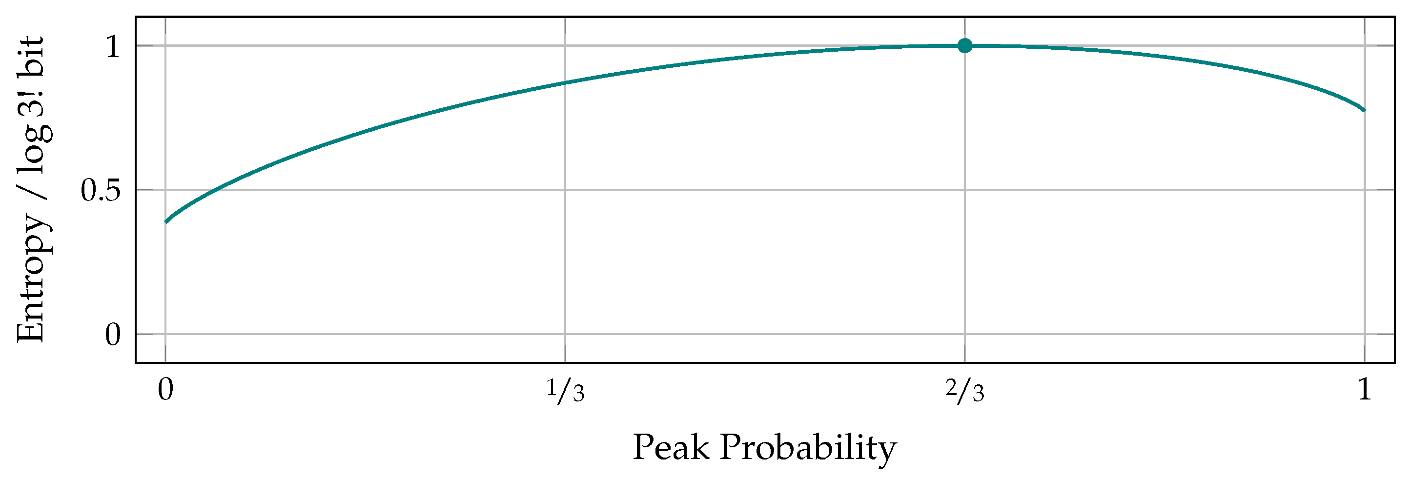
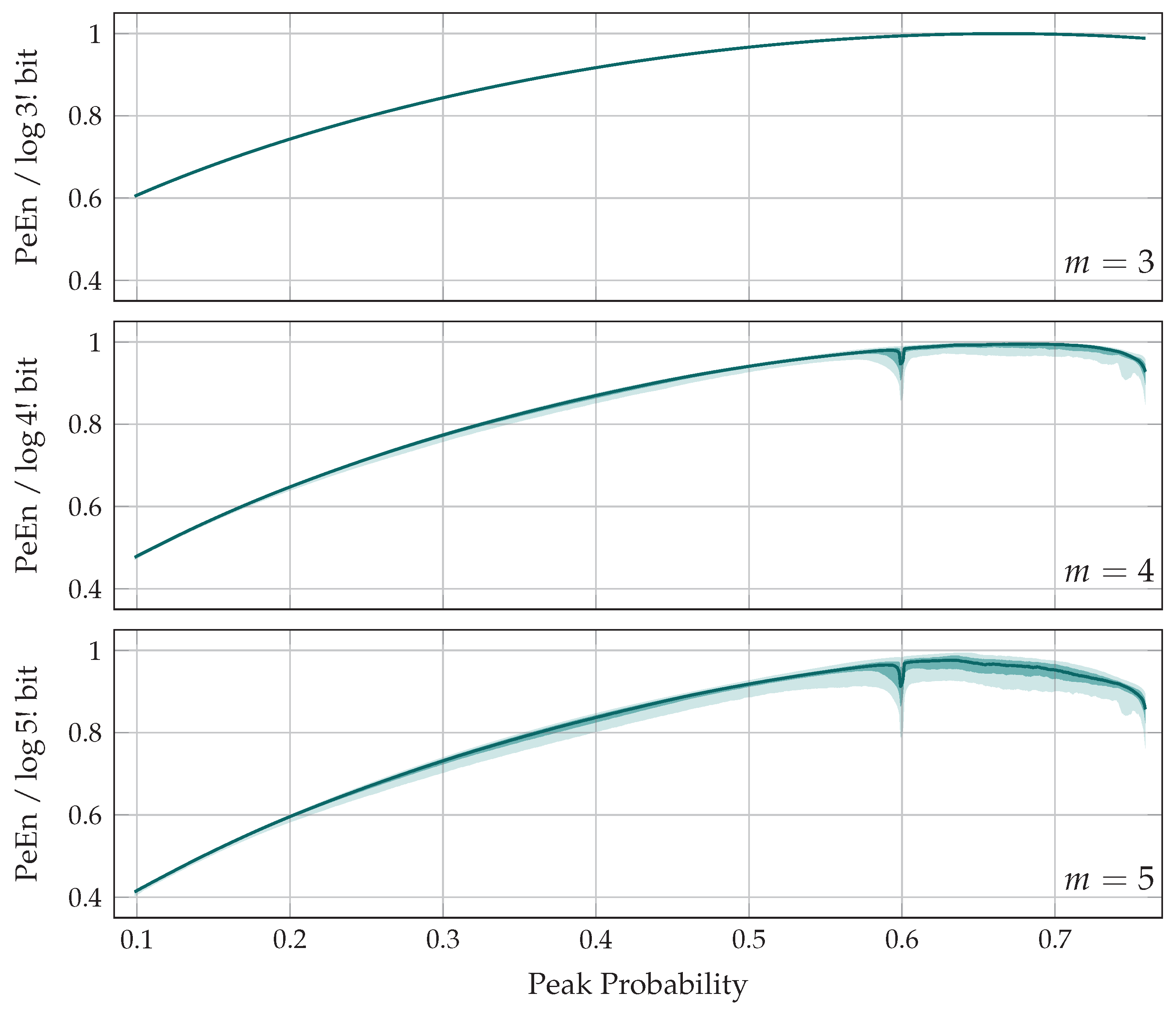
5. The Entropy of Peaks

The principle just demonstrated is directly transferable to actual PeEn. To this end, let us choose the six ordinal patterns of order m = 3 as a starting point. In addition, let us limit our considerations to the time delay τ = 1 for now—arbitrary time delays will be discussed near the end of the manuscript. We are thus looking at probability distributions of the form
p = p 123 p 132 p 213 p 231 p 312 p 321 T
and at their corresponding balance coefficients in terms of Equations (9) and (15),
β 123 / 123 β 123 / 132 β 123 / 213 β 123 / 231 β 123 / 312 β 123 / 321 β 132 / 123 β 132 / 132 β 132 / 213 β 132 / 231 β 132 / 312 β 132 / 321 β 213 / 123 β 213 / 132 β 213 / 213 β 213 / 231 β 213 / 312 β 213 / 321 β 231 / 123 β 231 / 132 β 231 / 213 β 231 / 231 β 231 / 312 β 231 / 321 β 312 / 123 β 312 / 132 β 312 / 213 β 312 / 231 β 312 / 312 β 312 / 321 β 321 / 123 β 321 / 132 β 321 / 213 β 321 / 231 β 321 / 312 β 321 / 321 .
Due to the symmetry relation of Equation (10), it suffices to consider the matrix entries above the main diagonal, that is, the coefficients β i j with 1 i < j 6 . We shall aggregate those 15 elements into a vector of balance coefficients
β = β 123 / 132 β 123 / 213 β 123 / 231 β 231 / 312 β 231 / 321 β 312 / 321 T .
Henceforth, we will use linear indexing, that is, the notation β i with 1 i 15 , when referring to the individual elements of the vector β .

5.1. An Open-Source, Open-Data Approach

The statistics of balance coefficients in EEG have to be assessed empirically, that is, from a suitably large collection of data. The analyses presented here were carried out on the CAP Sleep Database [12], a set of 108 polysomnographic recordings conducted at the Ospedale Maggiore di Parma, and kindly dedicated to the public domain. Sleep EEG data are particularly suitable for the task at hand: PeEn reportedly varies for different stages of natural sleep [8,13], and polysomnographic recordings usually encompass hours of contiguous data per subject. In addition, a multitude of pathologies justify polysomnographic clarification, which increases the heterogeneity of the data—another plus for our use case.
To aid reproducibility, using a dataset available to all of the scientific community was considered obligatory. The choice for the CAP Sleep Database was motivated by Bandt’s recent publication on PeEn [8]. The dataset is hosted by PhysioNet [14] and provided free of charge. Once more in the interest of reproducible science [15], the free and open-source numerical computation software GNU Octave 4.2 was utilised for all data analyses. The code is available in the supplementaries—and was tested compatible with MATLAB R2015b (MATLAB is a registered trademark of: The MathWorks, Inc., Natick, MA, USA).

5.2. EEG Segmentation and Processing

The CAP Sleep Database is a collection of 108 files stored in European Data Format (EDF) [16]. Four of them had to be rejected due to apparent inconsistencies in their file headers. From the remaining polysomnograms, all channels containing EEG were selected, irrespective of electrode location and referencing. These signals were converted to a common sampling rate of 200   Hz . No additional preprocessing nor any artefact correction were applied. The resampled EEG traces were then split into non-overlapping epochs of 20   s  duration each. To avoid biasing the ordinal pattern distributions, epochs containing ties (= triples of values that violate the constraint x 1 x 2 x 3 ) were discarded. The procedure yielded N cap = 1.6 × 10 6 individual segments—more than a year of (single-channel) EEG data.
Using the order  m = 3 and time delay  τ = 1 , epochs were then mapped onto sequences of ordinal patterns according to Equations (1) and (2). For each of the resulting N cap pattern sequences, its distribution vector
p i = p 123 i p 132 i p 213 i p 231 i p 312 i p 321 i T
was estimated in terms of Equation (4), and PeEn calculated as per Equation (5). Dividing by log m ! , results were normalised to the interval [ 0 , 1 ] . As is to be expected for sleep EEG, the data feature a wide range of PeEn values. Figure 4 depicts a density estimate of the non-trivially distributed entropy vector
h cap = h 1 h 2 h N cap T .

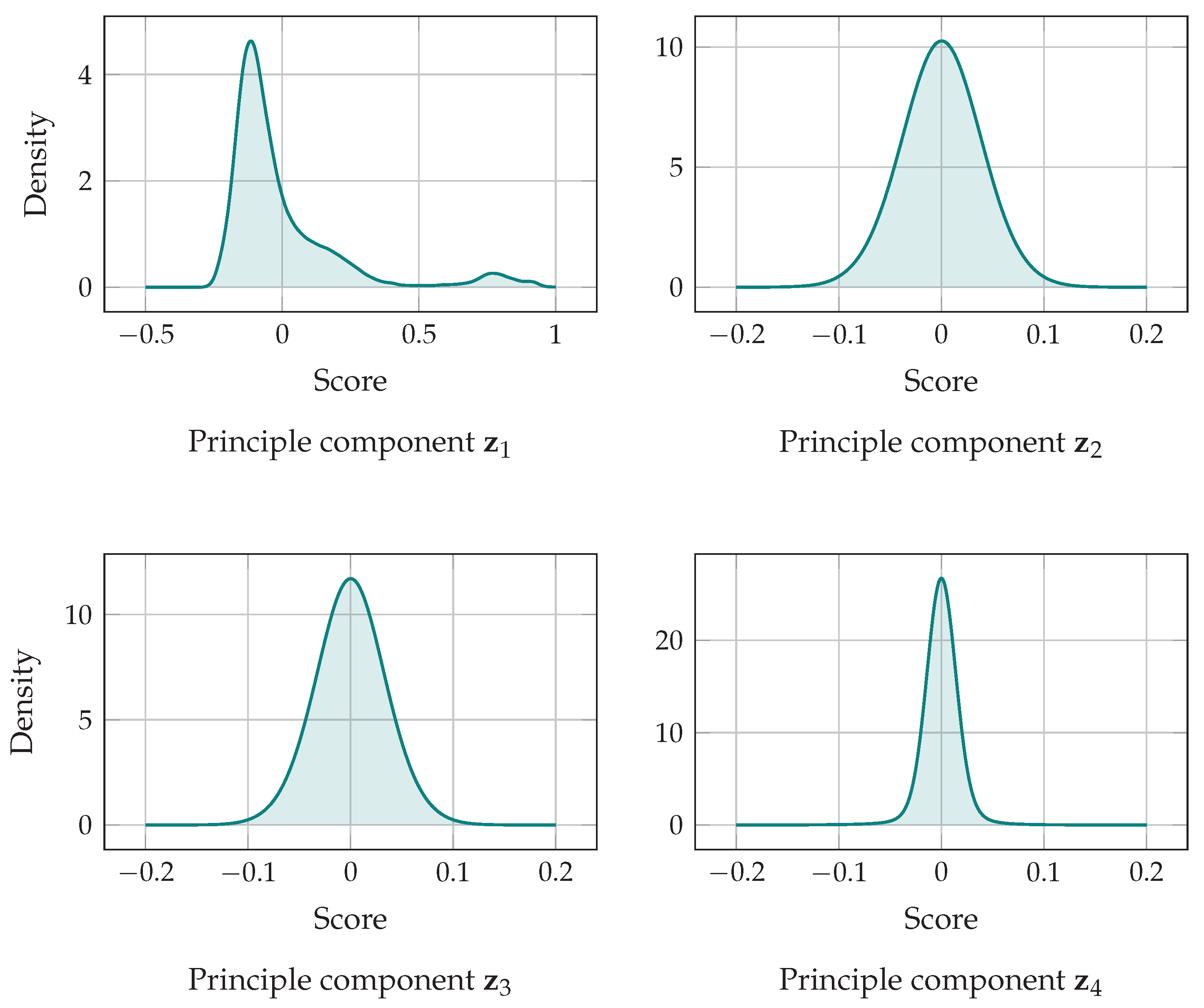
5.3. The Principle Components of Probability Balances

Furthermore, a vector of balance coefficients β i as per Equation (24) was computed for each ordinal pattern distribution p i . These vectors were concatenated to form the N cap × 15 data matrix
B = β 1 β 2 β N cap T .
Interpreting each vector β i (each row in B ) as one point in a 15-dimensional feature space, principle component analysis (PCA) was then carried out on the data matrix. This method constitutes a perfect match for the problem at hand, given that probability balance coefficients shall be ranked by their contribution to the overall variance in the data matrix B . Let us notate PCA in terms of computing the set of eigenpairs
( λ i , w i ) | 1 i 15
to the 15 × 15 covariance matrix  Σ B of the data matrix  B . The eigenvectors w i are then the loading vectors of the PCA and map B onto its principle components z i = B w i . Each principle component z i is a linear combination of the balance coefficients β i and explains a fraction of the variance in the dataset B , whereby it holds that λ i = Var ( z i ) . As is common practice, principle components shall be enumerated such that λ 1 λ 2 λ 15 . By convention, the first principle component z 1 then contributes most to the variance in B . For the actual CAP dataset, PCA revealed that
1 λ 0 i = 1 4 λ i > 0.999 with λ 0 = i = 1 15 λ i .
Thus, more than 99.9 % of variance in B are due to the principle components z 1 , z 2 , z 3 and z 4 (see Table 1). Further considerations were hence limited to the first four principle components. Their density estimates, as shown in Figure 5, are highly instructive.
The density of z 1 resembles the PeEn distribution depicted in Figure 4, suggesting some correlation between z 1 and the entropy values h cap . In contrast, the density estimates of z 2 , z 3 and z 4 seem to be normally distributed around zero—they appear to be random noise.
Testing for monotonic correlation between the PeEn values h cap and the principle components z 1 , z 2 , z 3 and z 4 , respectively, Spearman correlation coefficients as reported in Table 1 were obtained. Consistent with the graphical representations of Figure 4 and Figure 5, the first principle component z 1 is almost perfectly correlated with PeEn, while z 2 , z 3 and z 4 clearly contain uncorrelated noise. Moreover, z 1 alone explains more than 94 % of the variance in B . It is therefore safe to assume that the dynamics of PeEn are exclusively driven by z 1 .

5.4. Eliminating Pseudo-Complexity

The nature of the first principle component’s loading vector w 1 is the pivotal result of the manuscript at hand. According to the data presented in Table 2, it holds in very good approximation that
z 1 w 1 , 1 = β T w 1 w 1 , 1 β 123 / 132 β 123 / 213 β 123 / 231 β 123 / 312 β 132 / 321 β 213 / 321 β 231 / 321 β 312 / 321 T 1 1 1 1 1 1 1 1 = β 123 / 132 β 123 / 213 β 123 / 231 β 123 / 312 β 321 / 132 β 321 / 213 β 321 / 231 β 321 / 312 T 1 1 1 1 1 1 1 1 .
Here, the property of symmetry as per Equation (10) and a division by w 1 , 1 were applied to aid interpretability.
This is a bubble of pseudo-complexity bursting: while we were trying to isolate some pattern pairs that are irrelevant for the dynamics of PeEn in EEG, Equation (30) implies that the balances β i among all pattern pairs
Ω = ( 123 , 321 ) , ( 132 , 213 ) , ( 132 , 231 ) , ( 132 , 312 ) , ( 213 , 231 ) , ( 213 , 312 ) , ( 231 , 312 )
contribute virtually nothing to the variance in z 1 , and are thus negligible in good approximation. Those are the balances between any two peak patterns, as well as the balance β 123 / 321 between the all-rising and all-falling pattern.
Furthermore, estimating from data matrix B the mean, median and mode of each balance coefficient, results as presented in Table 2 were obtained. In particular, it holds true for all pattern pairs in Ω that
E [ β i ] Md [ β i ] Mo [ β i ] 1 / 2 ,
which strongly suggests that their respective balance coefficients are symmetrically distributed around  1 / 2 . Under this premise, and in conjunction with the definition as per Equation (9),
E [ p 123 ] E [ p 321 ] as well as E [ p 132 ] E [ p 213 ] E [ p 231 ] E [ p 312 ]
immediately follow. Moreover, and again due to the linear combination of Equation (30), the balance coefficients for the pattern pairs
Ω = { ( 123 , 132 ) , ( 123 , 213 ) , ( 123 , 231 ) , ( 123 , 312 ) , ( 321 , 132 ) , ( 321 , 213 ) , ( 321 , 231 ) , ( 321 , 312 ) }
contribute almost equally to the variance in B . These are the balances between any peak pattern and either the all-rising or all-falling pattern. Defining the peak probability p ^ such that
p ^ = p 132 + p 213 + p 231 + p 312 and 1 p ^ = p 123 + p 321 ,
and using the relations given in Equation (33), each of these balance coefficients can be approximated by
β = ( 1 p ^ ) / 2 ( 1 p ^ ) / 2 + p ^ / 4 = 2 ( p ^ 1 ) p ^ 2 .
The linear combination given by Equation (30) can therefore be reduced to the expression
z 1 w 1 , 1 8 β = 16 ( p ^ 1 ) p ^ 2 .
Let us assume that equality holds in the above relation, such that all variance within the decisive principle component z 1 is exclusively induced by the peak probability p ^ . Without compromising the dynamics of PeEn, all four peak patterns 132 , 213 , 231 and 312 can then be merged into just one ordinal pattern—the peak pattern. Likewise, the all-rising and all-falling patterns 123 and 321 can be unified, yielding a single edge pattern. On this basis, PeEn of order m = 3 and time delay τ = 1 can be replaced by a much simpler entropy of peaks function
H ( p ^ ) = p ^ log 4 p ^ + ( 1 p ^ ) log 2 1 p ^ = H b ( p ^ ) + p ^ log 2 + log 2 .
This function is concave with its maximum at p ^ = 2 / 3 , where p i = 1 / 6 for all i. The latter is consistent with Shannon entropy being maximal for the uniform distribution. The graph of H ( p ^ ) is depicted in Figure 6.
For the purpose of validation, H ( p ^ ) was calculated for all EEG epochs obtained from the CAP Sleep Database. Using the same overall approach as described in Section 5.2, but now computing the entropy of peaks according to Equations (35) and (38), a vector of N cap results h ^ cap was obtained. Comparison with the conventionally obtained PeEn values h cap yielded a Pearson correlation coefficient of r ( h cap , h ^ cap ) = 0.99998 and a mean relative error of
η ¯ ( h cap , h ^ cap ) = 1 N cap i = 1 N cap | h i h ^ i | h i = 0.03 % .
Thus, the ordinal patterns obtained from the CAP Sleep Database can essentially be replaced by binary symbols that encode the disjoint properties “three consecutive values form a peak” and “three consecutive values form an edge”.

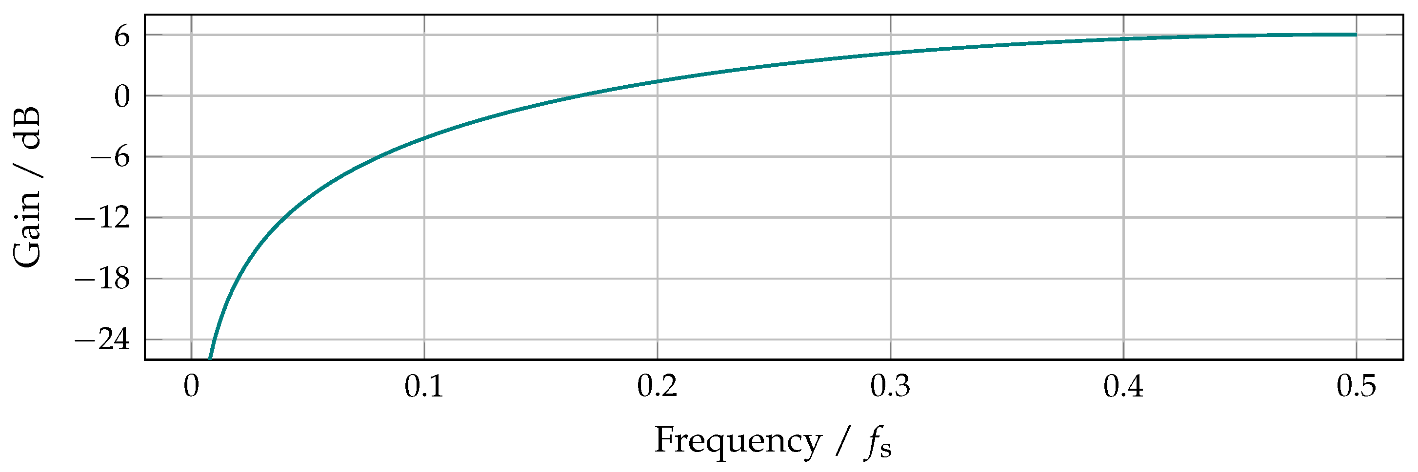
6. Linearising Permutation Entropy

At this point, we have substantiated the working hypothesis that, for EEG analysis, PeEn of order m = 3 may be a function of the peak probability p ^ only. This probability can be estimated from an epoch of n EEG samples ( x 1 , x 2 , , x n ) by computing
p ^ = n ^ n with n ^ = k = 2 n 1 x k x k 1 0 x k + 1 x k 0 ,
where the number of peaks n ^ is expressed using Iverson bracket notation [10]. Let us look in more detail at the properties of the decisive peak pattern.

6.1. Signal Peaks and Spectral Bandwidth

In mathematical terms, a peak is a local extremum. Any real-valued, twice differentiable function s has a peak at t k if it holds that s ( t k ) = 0 and s ( t k ) 0 . In other words, a peak in s is a zero crossing in its first derivative s . Now, consider a real-valued function s, periodic in T = 1 / f 0 and band limited to frequencies including N f 0 , which is
s ( t ) = k = 0 N a k sin ( 2 π k f 0 t + ϕ k ) with a k R .
Its first derivative is again a real-valued function, periodic in T and band limited to N f 0 , namely
s ( t ) = k = 0 N 2 π a k k f 0 cos ( 2 π k f 0 t + ϕ k ) = k = 0 N b k sin ( 2 π k f 0 t + ϑ k ) .
Being the N-th partial sum of a Fourier series, the function can alternatively be represented using complex exponentials,
s ( t ) = k = N N c k e j 2 π k f 0 t with j = 1 and c k C .
This expression constitutes a trigonometric polynomial of order N and therefore has exactly 2 N roots per period [17]. As for any real-valued polynomial, its zeroes
Z = t k | s ( t k ) = 0 , k 1 , 2 , , 2 N
are not necessarily distinct, and are either real or occur in complex conjugate pairs. Let us focus on the subset of zero crossings exclusively, which is
Z ø = t k R | s ( t k ) 0 Z .
With Z ø being a subset of Z, it obviously holds that | Z ø | 2 N . Furthermore, the number of peaks n ^ in the function s equals the number of zero crossings | Z ø | in its first derivative s . It therefore holds that
n ^ = | Z ø | 2 f max f 0 with f max = N f 0 .
Sampling one full cycle of the function s at a sampling rate of f s = n f 0 , we obtain a sequence of n values ( x 1 , x 2 , , x n ) . We can then express the maximum number of peaks per period by
n ^ 2 n f max f s with f max f s 2 .
Consequently, it holds for the peak probability p ^ that
p ^ = n ^ n 2 f max f s .
From a practical point of view, this relation is not limited to periodic signals. To assess f max in any signal segment, Fourier transform needs to be applied, which by definition constitutes a periodic continuation of the analysis window. Thus, the inequality given by Equation (48) provides an upper bound on the number of peaks in any band limited signal.
This bound may be naïvely conservative, but it is easily derived and suffices our purpose: let us reconsider the entropy of peaks function H ( p ^ ) as defined by Equation (38), which increases monotonically on the interval 0 p ^ 2 / 3 . In combination with Equation (48), this means that PeEn is monotonic with p ^ for EEG epochs band limited such that
f max f s 3 .
As stated earlier, the absolute value of PeEn obtained from a single EEG epoch is insignificant. It is the contrast in value across distinct epochs—its dynamics—that renders PeEn a valuable tool for EEG analysis. However, this contrast persists for any parameter that grows monotonically with PeEn. Therefore, the following constitutes an astounding, yet sensible proposition: given an epoch of EEG, digitised at sampling rate f s and band limited such that f max f s / 3 , PeEn of order m = 3 and time delay τ = 1 can be substituted by the peak probability p ^ , that is, the number of peaks per unit time.

6.2. Counting the Zigzags of EEG

For an experimental validation of the above, further EEG analyses were performed. To rule out possible peculiarities of the CAP Sleep Database (or sleep EEG in general), the data corpus was expanded by a set of EEG signals from a considerably different clinical setting. The CHB-MIT Scalp EEG Database is a collection of EEG recordings obtained from 22 paediatric patients, all suffering from epileptic seizures [18]. Acquired at Boston Children’s Hospital, the data were generously put into the public domain and are available from PhysioNet [14]. In strict analogy to the procedure described in Section 5.2, a total of N mit = 4.1 × 10 6 EEG epochs of 20   s  duration were obtained from this dataset—another two and a half years of (single-channel) EEG data. For each of these epochs, PeEn of order  m = 3 and time delay τ = 1 was computed according to Equations (1)–(6), yielding a vector of results  h mit .
From each EEG epoch of the CAP and CHB-MIT datasets, a peak probability p ^ as per Equation (40) was also obtained. Results were aggregated to form the respective vectors p ^ cap and p ^ mit . For both datasets, individual Spearman correlation coefficients between peak probabilities  p ^ and PeEn values  h were then computed for (1) the subset of EEG epochs with p ^ 2 / 3 , (2) the subset of EEG epochs with p ^ 2 / 3 , and (3) the entire set of epochs. Results are listed in Table 3.
The above results clearly support the hypothesis that PeEn of order m = 3 and time delay τ = 1 increases monotonically with the peak probability for p ^ 2 / 3 . The correlation is inverted for peak probabilities exceeding this bound. Both results are in line with the function graph of Figure 6. When testing on the full set of peak probabilities, strong positive correlation is maintained: epochs for which p ^ > 2 / 3 holds are too seldom to make a difference. This directly relates to the bandwidth constraint of Equation (49). Given our chosen sampling rate f s = 200   Hz , the peak probability cannot increase beyond p ^ = 2 / 3 for any EEG epoch band limited to frequencies below f max 66.7   Hz .
Not only is the relative bandwidth f max f s / 3 rarely exceeded in the datasets considered here, but the same presumably holds true for the vast majority of EEG in general. Sampling rates below 100   Hz are quite uncommon for EEG, while spectral content above 30   Hz is often regarded as insignificant (and actively suppressed using low-pass filtering). Moreover, an investigator actually interested in gamma-band oscillations will choose a considerably higher sampling rate. It is therefore likely that the decrease in PeEn for peak probabilities  p ^ > 2 / 3 is not a part of the actual effect, but a rarely observed flaw of the analysis technique. In essence, utilising PeEn of order m = 3 and time delay τ = 1 for EEG analysis may constitute an involved way of counting zigzags.

7. Permutation Entropy as a Spectral Estimator

While counting signal peaks may seem a trivial procedure at first glance, a profound mathematical theory supports this approach to signal analysis. It was formulated by Benjamin Kedem in the 1980s and is centred around the notion of higher order crossings. Only a humble outline of his framework—and one limited to aspects that aid the interpretation of PeEn—shall here be provided. For a large-scale, yet low-threshold introduction to the theory of higher order crossings, the reader is referred to Kedem’s comprehensive article “Spectral Analysis and Discrimination by Zero-Crossings” [19], which served as the primary source for the section to follow.

7.1. Zero Crossings and the Dominant Frequency Principle

Signal analysis by means of higher order crossings is a generalisation of the more commonly known zero crossing rate—a classic method of fundamental frequency estimation [20]. Self-descriptively, the zero crossing rate  r ø of a signal is its average number of x-intercepts per unit time. It is obtained from a discrete sequence of samples ( x 1 , x 2 , , x n ) by means of
r ø = n ø n 1 with n ø = i = 2 n x i 0 x i 1 0 .
Kedem refined the meaning of this quantity, demonstrating that the zero crossing rate of a discrete-time signal constitutes an approximation of the centroid of its power spectrum
c S = 1 m S 0 f S ( f ) d f with m S = 0 S ( f ) d f .
Here, S ( f ) denotes the power spectral density of the signal and m S is its (single-sided) spectral mass. Intuitively, if S ( f ) contains a predominant frequency f c , the spectral centroid c S will gravitate towards this particular frequency. The more S ( f c ) outweighs the rest of the spectrum, the shorter the distance between c S and f c will be. Kedem termed this the “dominant frequency principle”. Regarding its relation with the zero crossing rate, he further deduced that
r ø = n ø N 1 2 c S .
Maintaining the interdisciplinary scope of the article, we do not discuss the mathematical derivation of this relation—it can be found in [19]. Instead, a very conclusive example from the same publication shall be reproduced. Let our signal be the sinusoidal function s ( t ) = A sin ( 2 π f c t + φ ) , which has the power spectrum
S ( f ) = A 2 / 4 for f = ± f c , 0 otherwise .
With f c being the only frequency in the spectrum, it is obviously the dominant frequency. Calculating the spectral centroid of the signal, we see that the equality c S = f c holds true in this case. Hence, this example is a showcase for the dominant frequency principle. Moreover, and just as comprehensible, the relation
r ø = 2 f c = 2 c S
also applies: any sinusoidal signal has exactly two zero crossings per cycle.

7.2. Kedem’s Higher Order Crossings

Within the framework of higher order crossings, the peak probability p ^ of our simplified PeEn is closely related to the zero crossing rate r ø . Let ( x 1 , x 2 , , x n ) be a sequence of values sampled from a continuous-time EEG signal s ( t ) at discrete time steps t = i / f s = i T s . Estimating the peak probability p ^ of that sequence as per Equation (40) is equivalent to obtaining the zero crossing rate r ø of the difference sequence
( x 2 , x 3 , , x n ) ,
whereby the difference operator ∇ is defined such that
x i = x i x i 1 = s ( i T s ) s ( i T s T s ) .
In terms of Kedem’s theory, the generalised zero crossings obtained by applying the ∇-operator k times recursively are called: higher order crossings of the D k + 1 type. Thus, actual zero crossings are higher order crossings of the D 1 type, while the peak patterns considered in this manuscript are of type  D 2 .
Kedem’s approach is highly convenient in that the ∇-operator consitutes a linear time-invariant system with the power transfer function
| H ( f ) | 2 = | ( 1 e j 2 π f T s ) | 2 = 2 2 cos ( 2 π f T s ) .
This system acts as a high-pass filter in the digital domain. Its frequency response is depicted in Figure 7. In practical terms, the filter compresses the spectral mass, effectively shifting its centroid further to the right with each recurrent application of the ∇-operator.

7.3. The Spectral Estimation Hypothesis

We have now discussed all aspects necessary to propose an explanation for PeEn of order m = 3 and time delay τ = 1 in EEG. Let us summarise: due to their specific distribution in EEG, it may suffice to distinguish two kinds of ordinal patterns—peaks and edges. Their respective probabilities are p ^ and 1 p ^ . The peak probability p ^ is the zero crossing rate r ø of a high-pass filtered version of the signal, whereas the zero crossing rate r ø is an estimate of its power spectral centroid. For EEG epochs with p ^ 2 / 3 , the peak probability p ^ and PeEn are monotone and can therefore be used interchangeably in comparative analyses.
On that basis, it is a rational hypothesis that applying PeEn of order m = 3 and time delay τ = 1 to EEG epochs with peak probability p ^ 2 / 3 effectively means: high-pass filtering the signal according to Equation (57) and estimating the centroid of the resulting weighted power spectrum. Both steps are standard procedures of linear signal processing, possibly rendering this EEG parameter a spectral estimator in disguise.

8. Higher Pattern Orders and Time Delays

Throughout the manuscript, considerations and propositions were repeatedly limited to the pattern order m = 3 and the time delay τ = 1 . Regarding the latter, a general discussion was postponed for reasons of simplicity only. It will be presented in the following section. Conversely, formulating a universal interpretation for pattern orders m > 3 is a subject still under investigation—and hopefully one to be reported on in the future. For the time being, the reader is invited to consider the following preliminary results.

8.1. Prospects for Patterns of Higher Order

An ordinal pattern of order m = 3 is either a peak or an edge. For higher orders, there is no such simple duality. In the general case, an ordinal pattern of order m can contain up to m 2 peaks, while the peaks of consecutive ordinal patterns may overlap. Moreover, the marginal probability relation of Equation (33) does not translate to the “sub-patterns” of order m = 3 that form a pattern of higher order. Conditional probabilities have to be considered instead.
Despite such intricacies, the principle behaviour of PeEn does apparently not change when increasing the order m within statistically reasonable limits. Calculating PeEn of orders m { 3 , 4 , 5 } for all EEG epochs obtained from the CAP and CHB-MIT datasets, results as depicted in Figure 8 were obtained. Strong monotonic correlation between PeEn and the peak probability p ^ is maintained for higher pattern orders. This hints at a possible generalisation of our spectral estimation hypothesis.

8.2. Sampling, Resampling and Aliasing

In comparison to higher pattern orders m, interpreting arbitrary time delays  τ is straightforward. Under the premise that PeEn acts as a spectral estimator in EEG analysis, the principles of linear systems theory fully apply. Using time delays τ > 1 is then a means of downsampling (and thus, of band limiting), but also constitutes a violation of the Nyquist–Shannon sampling theorem. Let us substantiate.
The Nyquist–Shannon sampling theorem [21] states that any time-discrete representation of an analogue signal is implicitly band limited to frequencies below and including half its sampling rate f s . Due to this fundamental constraint of digital signal processing, an analogue low-pass filter is commonly applied during signal acquisition. This filter prevents distortions known as aliasing—spectral content beyond the Nyquist frequency f s / 2 folding back into the usable frequency range as given by the mapping
f f s 2 | ( f mod f s ) f s 2 | with f 0 .
This relation describes a triangle waveform with its extrema at multiples of f s / 2 . Its graph is displayed in Figure 9.
The same constraint applies to sampling rate conversion in the digital domain. Correctly reducing the sampling rate f s of a digital signal by a factor r therefore involves two steps: limit the bandwidth to f s / 2 r , then omit all but every r-th sample. If the band limiting is skipped, downsampling is prone to aliasing. Any spectral content exceeding f s / 2 r is not compatible with the targeted sampling rate f s / r and folds back into the representable frequency range, corrupting the resulting signal.

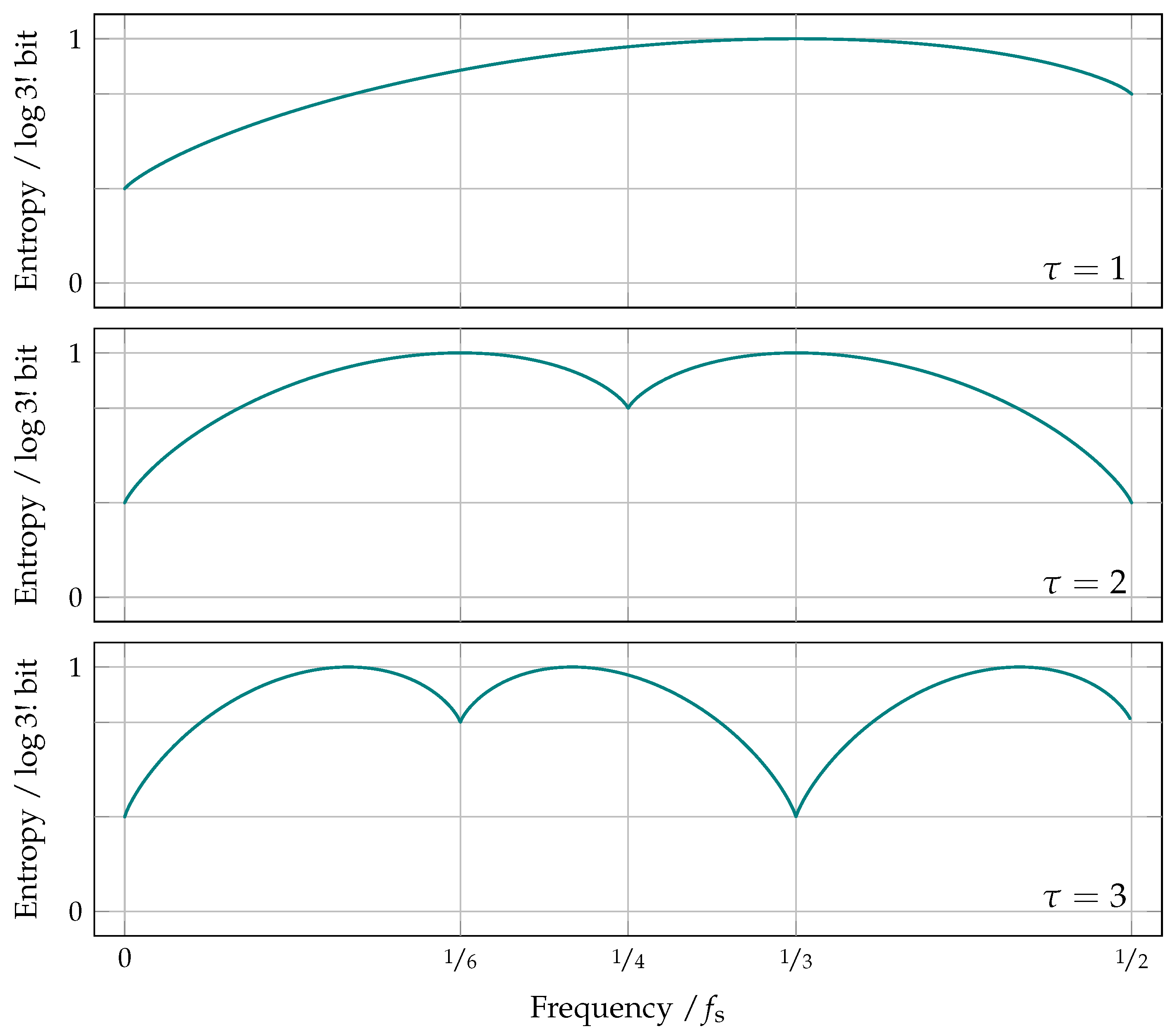
8.3. The Time Delay as a Downsampling Factor

Let us look again at what is called the symbolisation technique. Given a sequence of samples ( x 1 , x 2 , , x n ) , its ordinal pattern π t of order m and time delay  τ at time index t is obtained from the m-tuple of values
( x t , x t + τ , x t + 2 τ , , x t + ( m 1 ) τ ) .
To estimate the ordinal pattern distribution of the sequence, we determine π t for 1 t n τ ( m 1 ) and count the number of occurrences of each pattern Π i Ω m . This is the method described by Equations (1)–(4).
For  τ > 1 , consider an alternative, yet entirely equivalent estimation algorithm: first, partition the sequence of samples ( x 1 , x 2 , , x n ) into τ sub-sequences of the form
λ { 1 , 2 , , τ } : ( x λ , x λ + τ , x λ + 2 τ , , x λ + k τ ) whereby k = n λ τ + 1 .
Next, estimate from each of the τ sub-sequences its ordinal pattern distribution p λ , now using the time delay τ = 1 . The ordinal pattern distribution p of the initial sequence can then be obtained by cumulation, that is
p = λ = 1 τ p λ = p 1 + p 2 + + p τ .
Observe that generating a sub-sequence as per Equation (60) is identical to downsampling the sequence ( x 1 , x 2 , , x n ) by a factor τ (whereby the index λ merely specifies which sample to keep per block of τ consecutive samples). This circumstance is both the explanation and the fundamental problem of using τ > 1 for ordinal pattern encoding: we implicitly—but no less effectively—downsample the signal without any anti-aliasing measures taken. Inevitably, all spectral content exceeding f s / 2 τ folds back into the representable frequency range. Therefore, calculating PeEn from EEG using τ > 1 is equivalent to computing PeEn for the time delay τ = 1 from a set of τ downsampled (and therefore band limited), yet nonlinearly distorted versions of the actual signal.
Notice that this is not a conceptual flaw of PeEn. One has to keep in mind that the quantity was developed as a complexity measure for time series. Working with less generic data, additional constraints and requirements may arise. In particular, while any digital signal can be described as a time series, not all time series are digital signals in terms of linear systems theory. Only if the requirements of the sampling theorem are adhered to can a discrete sequence of voltage measurements be a valid representation of analogue EEG.

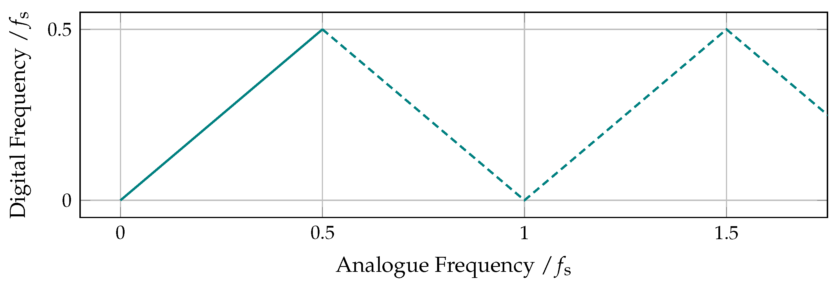
8.4. Frequency Aliasing in Permutation Entropy

Computing the entropy of peaks H ( p ^ ) as per Equation (38) from sinusoidal signals of varying frequency  f c f s / 2 , the aliasing introduced by using time delays τ > 1 is easily observed. In accordance with the frequency mapping of Equation (58), and depending on the effective sampling rate f s / τ , the signal that is actually fed into the estimator is a sinusoidal wave of frequency
f c ˜ = f s 2 τ | ( f c mod f s τ ) f s 2 τ | .
Given that any sinusoidal signal has exactly two peaks per cycle, it further holds that p ^ = 2 f c ˜ . In conjunction with Equation (38), the relation
H ( p ^ ) = H ( 2 f c ˜ ) = H b ( 2 f c ˜ ) + 2 f c ˜ log 2 + log 2
is obtained. Variegating the time delay τ , the periodic foldback effect manifests in the graphs of this family of functions. This is depicted and further discussed in Figure 10.
The presented approach is based on the work of Erik Olofsen, Jamie Sleigh and Albert Dahan. To experimentally investigate the frequency dependence of PeEn, the authors calculated PeEn of order m = 3 and time delays τ 2 for sinusoidal signals of increasing frequency [22]. Our here proposed spectral estimation hypothesis conclusively explains the authors’ observations, including the discontinuous frequency dependence for τ = 2 .

8.5. Anti-Aliased Permutation Entropy

Using time delays τ > 1 for EEG encoding may cause unintended signal distortions. Nevertheless, a multitude of applications in EEG analysis depend on higher time delays [11]. In practice, the impact of aliasing may be less detrimental than the graphs of Figure 10 suggest: EEG is anything but sinusoidal, and while PeEn literally locks onto a single sine wave, the discrepancy will be more subtle for actual EEG. In addition, EEG is commonly oversampled ( f s 2 f max ), which further mitigates the issue (see Section 6).
Nothing is lost by resolving a source of inaccuracy, though. This is easily achieved by means of sample rate conversion. A possible procedure is as follows: instead of using τ > 1 for PeEn calculation, correctly convert the EEG to a new sampling rate f s = f s / τ and compute PeEn therefrom, now choosing τ = 1 for the time delay. An apparent disadvantage of this approach is that it reduces the number of ordinal patterns available for probability estimation by a factor τ . However, the sampling theorem implicitly assures that a single rate-reduced sequence suffices to fully describe the band limited EEG—including its signal peaks. Nothing is gained by counting each peak τ times.
In the anti-aliased case, a very tangible interpretation of the time delay  τ immediately follows: PeEn effectively splits the signal’s single-sided frequency spectrum into τ  spectral bands of equal width, then exclusively responds to the content of the lowest band. Given our spectral estimation hypothesis, PeEn of order m = 3 and time delay τ 1 thus approximates the weighted power spectral centroid of the EEG’s frequency band ranging from 0 to  f s / 2 τ . For applications depending on τ > 1 , it may hence be worthwhile to further investigate the influence of anti-aliasing. This could be a chance of concisely relating PeEn-based techniques with classic band-spectral methods of EEG analysis.

9. Conclusions

EEG has long become an indispensable tool in research and medical diagnostics, even more so as the progress in digital technology has revolutionised our general approach towards data—biomedical data being no exception.

9.1. There Are Only So Many Signal Characteristics

When analysing EEG, one has to accept its predominantly probabilistic nature. Any signal property that statistically correlates with some behavioural observation is a perfectly valid signal property because, ultimately, none of them are fully explainable mechanistically. While a plethora of EEG analysis techniques are available, the application of a new or more sophisticated method does not necessarily yield new information: analysing the EEG data considered for this manuscript, (1) PeEn of order m = 3 and time delay τ = 1 ; (2) the power spectral centroid of the signal’s first derivative; and (3) Kedem’s higher order crossings of the D 2 type can all be used interchangeably.
The signal property apparently underlying all three methods has been known and used for more than 50 years now. In 1964, Neil Burch and colleagues reported on transferring the EEG analysis method of counting “baseline crossing[s]” from analogue circuitry to a digital computer [23]. The authors explicitly pointed out the “well-known accentuation of the higher frequency component in the derivatives”. Back then, the procedure was called period analysis.

9.2. Next Steps in Ordinal Pattern-Based EEG Analysis

It cannot be over-emphasized that EEG analysis is mostly empirical—including the results of this manuscript. What applies for the CAP and CHB-MIT databases does not necessarily hold true for EEG in general. Hence, the work presented does neither falsify the existence of complexity in EEG, nor its observability using PeEn. Still, it demonstrates that PeEn-based EEG processing does not exclusively relate to this phenomenon.
This article thus extends the framework of ordinal pattern-based EEG processing. For a given analysis task, concurrently computing both PeEn and the peak probability  p ^ provides a means of rejecting the null hypothesis of PeEn acting as a spectral estimator. This may enable the investigator to narrow down on cases that truly demand for complexity considerations, while otherwise resorting to a simpler and time-tested analysis technique. To this end, the peak probability  p ^ as specified by Equation (40) integrates seamlessly into the framework of ordinal pattern analysis. A convenient side effect: if for a particular analysis task PeEn is found to be replaceable by p ^ , the issue of pattern order selection does not arise.
In closing, adding the peak probability parameter to your codebase is straightforward. The expression
y = mean ( abs ( diff ( diff ( x ) > = 0 ) ) ) ;
suffices to have the quantity available within a GNU Octave or MATLAB environment. An extended version that supports sliding window analysis is provided in the supplementaries (see the zztop.m function). While not extensively optimised, its execution speed should meet the requirements of major analysis campaigns: the main challenge in data analysis today is not computational feasibility, but the interpretation of the manifold results obtainable.

Supplementary Materials

The GNU Octave/MATLAB code used is available online at www.mdpi.com/1099-4300/19/12/692/s1 and www.github.com/seb-berger/zztop.

Acknowledgments

All authors thank the anonymous reviewers for their constructive suggestions. Sebastian Berger thanks Kristine Kellermann, Andrii Kravtsiv, Andreas Ranft and Claudia Scheffzük for valuable exchange. This work was in part supported by the Bundesministerium für Bildung und Forschung (BMBF, VIP03V0502). This work was supported by the Deutsche Forschungsgemeinschaft (DFG) and the Technische Universität München (TUM) in the framework of the Open Access Publishing Program.

Author Contributions

Sebastian Berger conceived the approach and performed the analyses; Denis Jordan supervised the analysis process; all authors interpreted and discussed intermediate and final results; Sebastian Berger prepared the manuscript; Gerhard Schneider, Eberhard F. Kochs and Denis Jordan revised the manuscript; all authors have read and approved the final version of the manuscript.

Conflicts of Interest

The authors declare no conflict of interest.

References

  1. Bandt, C.; Pompe, B. Permutation Entropy: A Natural Complexity Measure for Time Series. Phys. Rev. Lett. 2002, 88, 174102. [Google Scholar] [CrossRef] [PubMed]
  2. Zanin, M.; Zunino, L.; Rosso, O.A.; Papo, D. Permutation Entropy and Its Main Biomedical and Econophysics Applications: A Review. Entropy 2012, 14, 1553–1577. [Google Scholar] [CrossRef]
  3. Amigó, J.M.; Keller, K.; Unakafova, V.A. Ordinal symbolic analysis and its application to biomedical recordings. Phil. Trans. R. Soc. A 2014, 373, 20140091. [Google Scholar] [CrossRef] [PubMed]
  4. Fadlallah, B.; Chen, B.; Keil, A.; Príncipe, J. Weighted-permutation entropy: A complexity measure for time series incorporating amplitude information. Phys. Rev. E 2013, 87, 022911. [Google Scholar] [CrossRef] [PubMed]
  5. Li, D.; Li, X.; Liang, Z.; Voss, L.J.; Sleigh, J.W. Multiscale permutation entropy analysis of EEG recordings during sevoflurane anesthesia. J. Neural Eng. 2010, 7, 046010. [Google Scholar] [CrossRef] [PubMed]
  6. Morabito, F.C.; Labate, D.; La Foresta, F.; Bramanti, A.; Morabito, G.; Palamara, I. Multivariate Multi-Scale Permutation Entropy for Complexity Analysis of Alzheimer’s Disease EEG. Entropy 2012, 14, 1186–1202. [Google Scholar] [CrossRef]
  7. Azami, H.; Escudero, J. Amplitude-aware Permutation Entropy: Illustration in Spike Detection and Signal Segmentation. Comput. Methods Progr. Biomed. 2016, 128, 40–51. [Google Scholar] [CrossRef] [PubMed]
  8. Bandt, C. A New Kind of Permutation Entropy Used to Classify Sleep Stages from Invisible EEG Microstructure. Entropy 2017, 19, 197. [Google Scholar] [CrossRef]
  9. Shannon, C.E. A Mathematical Theory of Communication. Bell Syst. Tech. J. 1948, 27, 379–423. [Google Scholar] [CrossRef]
  10. Iverson, K.E. A Programming Language. In Proceedings of the Spring Joint Computer Conference, AIEE-IRE ’62 (Spring), San Francisco, CA, USA, 1–3 May 1962; ACM: New York, NY, USA, 1962; pp. 345–351. [Google Scholar]
  11. Riedl, M.; Müller, A.; Wessel, N. Practical considerations of permutation entropy. Eur. Phys. J. Spec. Top. 2013, 222, 249–262. [Google Scholar] [CrossRef]
  12. Terzano, M.G.; Parrino, L.; Sherieri, A.; Chervin, R.; Chokroverty, S.; Guilleminault, C.; Hirshkowitz, M.; Mahowald, M.; Moldofsky, H.; Rosa, A.; et al. Atlas, rules, and recording techniques for the scoring of cyclic alternating pattern (CAP) in human sleep. Sleep Med. 2001, 2, 537–553. [Google Scholar] [CrossRef]
  13. Nicolaou, N.; Georgiou, J. The Use of Permutation Entropy to Characterize Sleep Electroencephalograms. Clin. EEG Neurosci. 2011, 42, 24–28. [Google Scholar] [CrossRef] [PubMed]
  14. Goldberger, A.L.; Amaral, L.A.N.; Glass, L.; Hausdorff, J.M.; Ivanov, P.C.; Mark, R.G.; Mietus, J.E.; Moody, G.B.; Peng, C.K.; Stanley, H.E. PhysioBank, PhysioToolkit, and PhysioNet: Components of a New Research Resource for Complex Physiologic Signals. Circulation 2000, 101, e215–e220. [Google Scholar] [CrossRef] [PubMed]
  15. Eaton, J.W. GNU Octave and reproducible research. J. Process Control 2012, 22, 1433–1438. [Google Scholar] [CrossRef]
  16. Kemp, B.; Värri, A.; Rosa, A.C.; Nielsen, K.D.; Gade, J. A simple format for exchange of digitized polygraphic recordings. Electroenceph. Clin. Neurophysiol. 1992, 82, 391–393. [Google Scholar] [CrossRef]
  17. Requicha, A.A.G. The Zeros of Entire Functions: Theory and Engineering Applications. Proc. IEEE 1980, 68, 308–328. [Google Scholar] [CrossRef]
  18. Shoeb, A.H. Application of Machine Learning to Epileptic Seizure Onset Detection and Treatment. Ph.D. Thesis, Massachusetts Institute of Technology, Cambridge, MA, USA, 2009. [Google Scholar]
  19. Kedem, B. Spectral Analysis and Discrimination by Zero-Crossings. Proc. IEEE 1986, 74, 1477–1493. [Google Scholar] [CrossRef]
  20. Rice, S.O. Statistical Properties of a Sine Wave Plus Random Noise. Bell Syst. Tech. J. 1948, 27, 109–157. [Google Scholar] [CrossRef]
  21. Shannon, C. Communication in the Presence of Noise. Proc. IRE 1949, 37, 10–21. [Google Scholar] [CrossRef]
  22. Olofsen, E.; Sleigh, J.W.; Dahan, A. Permutation entropy of the electroencephalogram: A measure of anaesthetic drug effect. Br. J. Anaesth. 2008, 101, 810–821. [Google Scholar] [CrossRef] [PubMed]
  23. Burch, N.R.; Nettleton, W.J.; Sweeney, J.; Edwards, R.J. Period analysis of the electroencephalogram on a general-purpose digital computer. Ann. N. Y. Acad. Sci. 1964, 115, 827–843. [Google Scholar] [CrossRef] [PubMed]
Figure 1. A schematical representation of the six ordinal patterns of order m = 3 .
Entropy 19 00692 g001
Figure 2. The graph of H Δ as specified by Equation (14), calculated using the binary logarithm. The function is symmetrical to the plane β i j = 1 / 2 , where it is maximal with regard to β i j for any constant p i j . H Δ is then an affine transformation of the binary entropy function H b . It is the binary entropy function for p i j = 1 .
Entropy 19 00692 g002
Figure 3. The twelve extra-ordinal patterns of order m = 3 . Highlighted samples are pivotal in that they render a pattern top-heavy ( t ) or bottom-heavy ( b ). Each pattern pair Π t i and Π b i descends from a common ordinal pattern Π i .
Entropy 19 00692 g003
Figure 4. Kernel density estimate (Gaussian, bandwidth σ = 5 × 10 3 ) for the N cap = 1.6 × 10 6 PeEn values obtained from the CAP Sleep Database.
Entropy 19 00692 g004
Figure 5. Kernel density estimates (Gaussian, bandwidth σ = 1 × 10 2 ) for the principle components z 1 , z 2 , z 3 and z 4 of the data matrix B .
Entropy 19 00692 g005
Figure 6. The entropy of peaks function H ( p ^ ) of Equation (38), divided by log 3 ! for normalisation. The maximum is taken on for p ^ = 2 / 3 , where H ( p ^ ) = 1 .
Entropy 19 00692 g006
Figure 7. Power transfer function | H ( f ) | 2 of the ∇-operator for frequencies including the Nyquist rate.
Entropy 19 00692 g007
Figure 8. Solid curves represent the median of permutation entropy (PeEn), plotted with regard to the peak probability. Where graphically representable, inner shaded bands correspond to the 25th–75th, outer shaded bands to the 5th–95th percentiles. Peak probabilities occurring less than 100 times were discarded and missing values linearly interpolated. A moving average filter of bandwidth 2.5 × 10 3 was applied for data smoothing.
Entropy 19 00692 g008
Figure 9. The aliasing relation as specified by Equation (58). Any spectral content exceeding the Nyquist rate f ny = f s / 2 is periodically folded back into the representable frequency range.
Entropy 19 00692 g009
Figure 10. The entropy of peaks function H ( p ^ ) calculated from a sine wave of increasing frequency. For the time delay τ = 1 , the function behaves as discussed for Figure 6. When using time delays τ > 1 , aliasing is provoked for frequencies exceeding f s / 2 τ . Those frequencies periodically fold back into the representable spectrum, which leads to symmetries in PeEn.
Entropy 19 00692 g010
Table 1. Eigenvalues and explained variations (normalised eigenvalues) of the first four principle components, as well as their Spearman correlation coefficients with the permutation entropy (PeEn) vector h cap .
Component z i Eigenvalue λ i Explained Variation λ i / λ 0 Spearman Correlation ρ ( h cap , z i )
z 1 5.0 × 10 2 94.4 % 0.99996
z 2 1.5 × 10 3 2.8 % 0.006
z 3 1.2 × 10 3 2.2 % 0.008
z 4 2.5 × 10 4 0.5 % 0.02
Table 2. The principle component z 1 = β T w 1 is a (trivially simple) linear combination of a subset of balance coefficients. In addition, all balance coefficients not included in z 1 (listed in the lower part of the table) appear to be symmetrically distributed around 1 / 2 .
Index i Balance β i WeightMean E [ β i ] Media Md [ β i ] Mode Mo [ β i ]
w 1 , i w 1 , i / w 1 , 1
1 β 123 / 132 0.353 1.000 0.8588 0.8842 0.9000
2 β 123 / 213 0.354 1.002 0.8586 0.8842 0.9000
3 β 123 / 231 0.353 0.999 0.8588 0.8842 0.9000
4 β 123 / 312 0.352 0.997 0.8590 0.8842 0.9000
9 β 132 / 321 0.354 1.003 0.1415 0.1157 0.0909
12 β 213 / 321 0.355 1.005 0.1417 0.1158 0.0909
14 β 231 / 321 0.354 1.002 0.1414 0.1158 0.1111
15 β 312 / 321 0.353 1.000 0.1412 0.1158 0.0909
5 β 123 / 321 0.002 0.005 0.5004 0.5004 0.5000
6 β 132 / 213 0.001 0.003 0.4997 0.5000 0.5000
7 β 132 / 231 0.001 0.001 0.5001 0.5000 0.5000
8 β 132 / 312 0.001 0.004 0.5004 0.5000 0.5000
10 β 213 / 231 0.001 0.004 0.5004 0.5000 0.5000
11 β 213 / 312 0.002 0.007 0.5007 0.5008 0.5000
13 β 231 / 312 0.001 0.003 0.5003 0.5000 0.5000
Table 3. Spearman correlation coefficients between PeEn values h and peak probabilities p ^ for the electroencephalographic data from the CAP Sleep Database and the CHB-MIT Scalp EEG Database. Quantities subscripted “high” and “low” correspond to results obtained from those subsets of signal epochs for which p ^ 2 / 3 or p ^ 2 / 3 hold, respectively.
DatabaseNumber of EpochsSpearman Correlation
N N low N high ρ ( h , p ^ ) ρ low ( h , p ^ ) ρ high ( h , p ^ )
CAP 1.6 × 10 6 1.6 × 10 6 6.0 × 10 2 0.99998 0.99998 0.923
CHB-MIT 4.1 × 10 6 4.0 × 10 6 1.1 × 10 5 0.99937 0.99993 0.963

