Information Theory to Probe Intrapartum Fetal Heart Rate Dynamics


Abstract
1. Introduction
2. Datasets: Intrapartum Fetal Heart Rate Times Series and Labor Stages
3. Methods
3.1. Information Theory Features
3.1.1. Shannon and Rényi Entropies
3.1.2. Entropy Rates
3.1.3. Mutual Information
3.2. Features from Complexity Theory
3.2.1. Approximate Entropy
3.2.2. Sample Entropy
3.2.3. Estimation
3.3. Connecting Complexity Theory and Information Theory
3.3.1. Limit of Large Datasets and Vanishing : Exact Relation
3.3.2. New Features
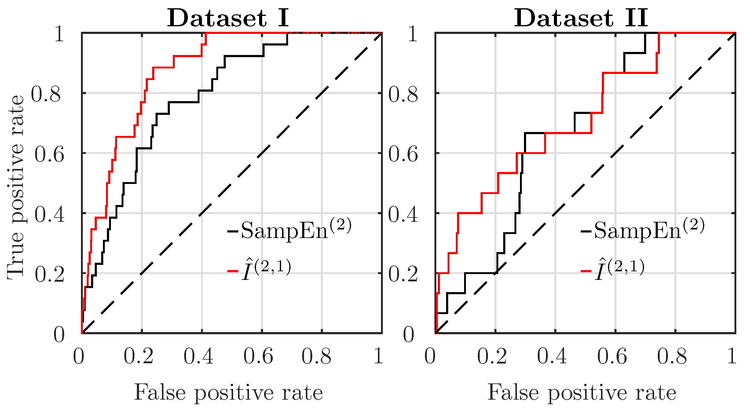
4. Results: Acidosis Detection Performance
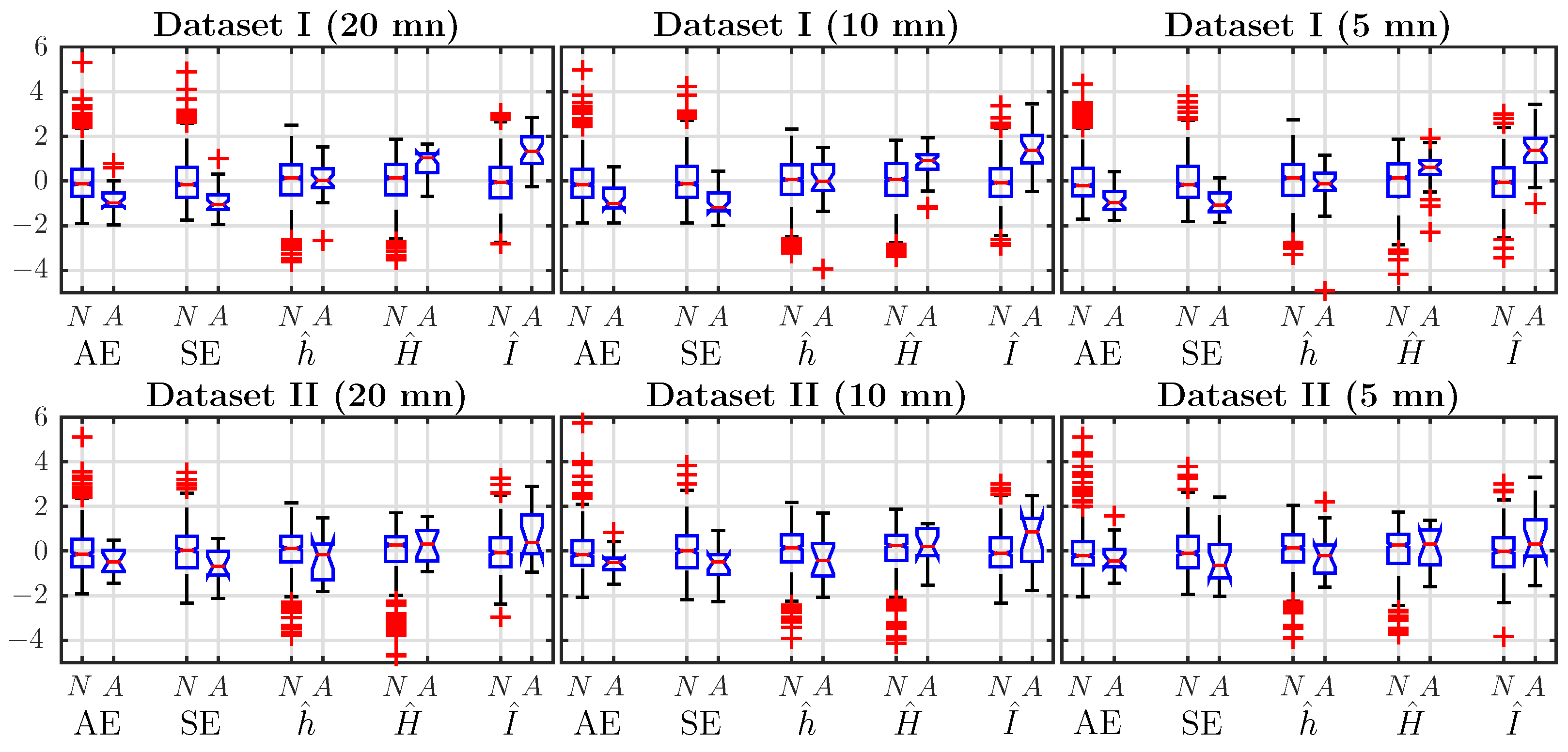
4.1. Comparison of Features’ Performance, Using a Single Time Window, Just Before Delivery
4.2. Effect of Window Size on Performance
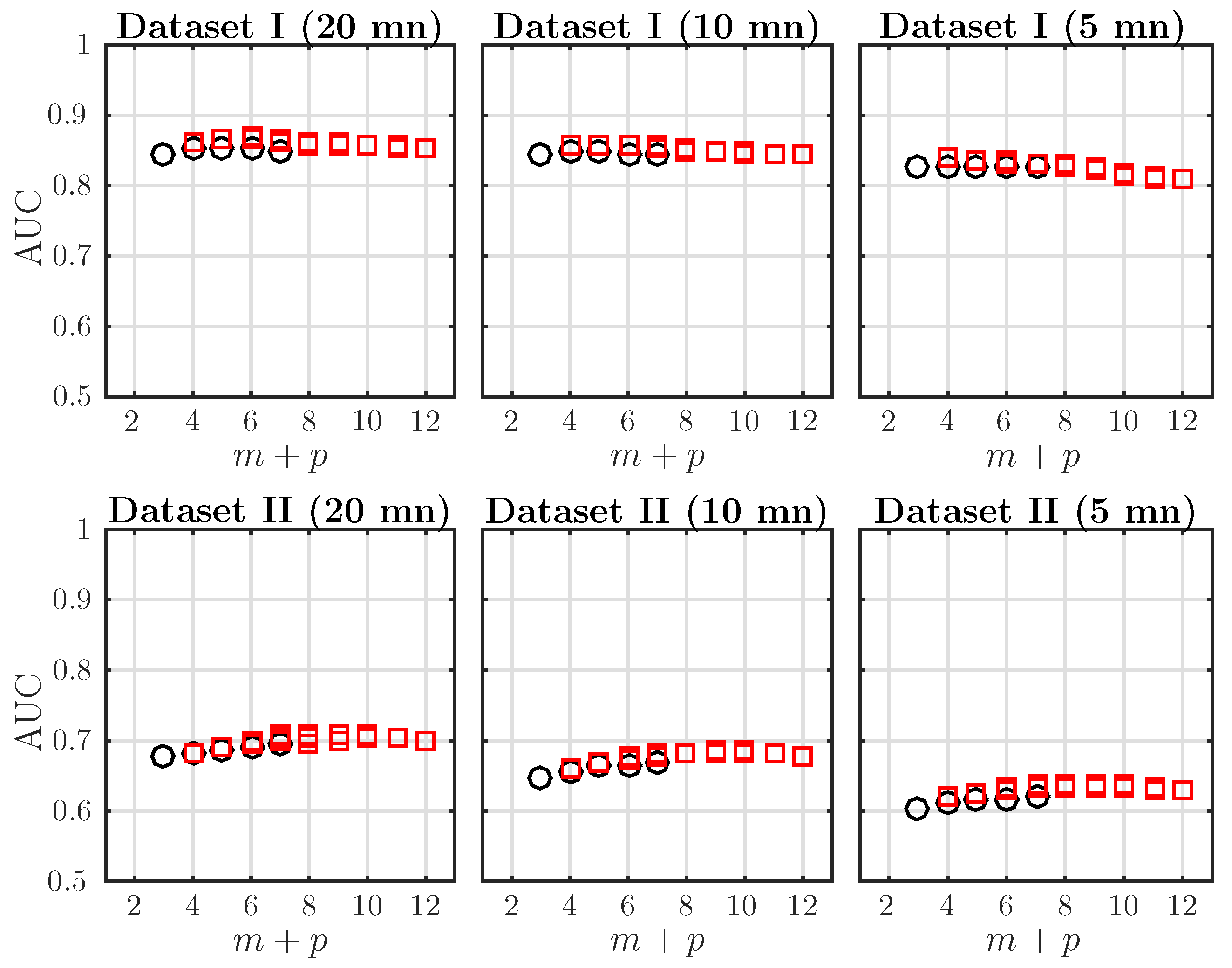
4.3. Effect of the Embedding Dimensions on the (Fetal Acidosis Detection) Performance of AMI
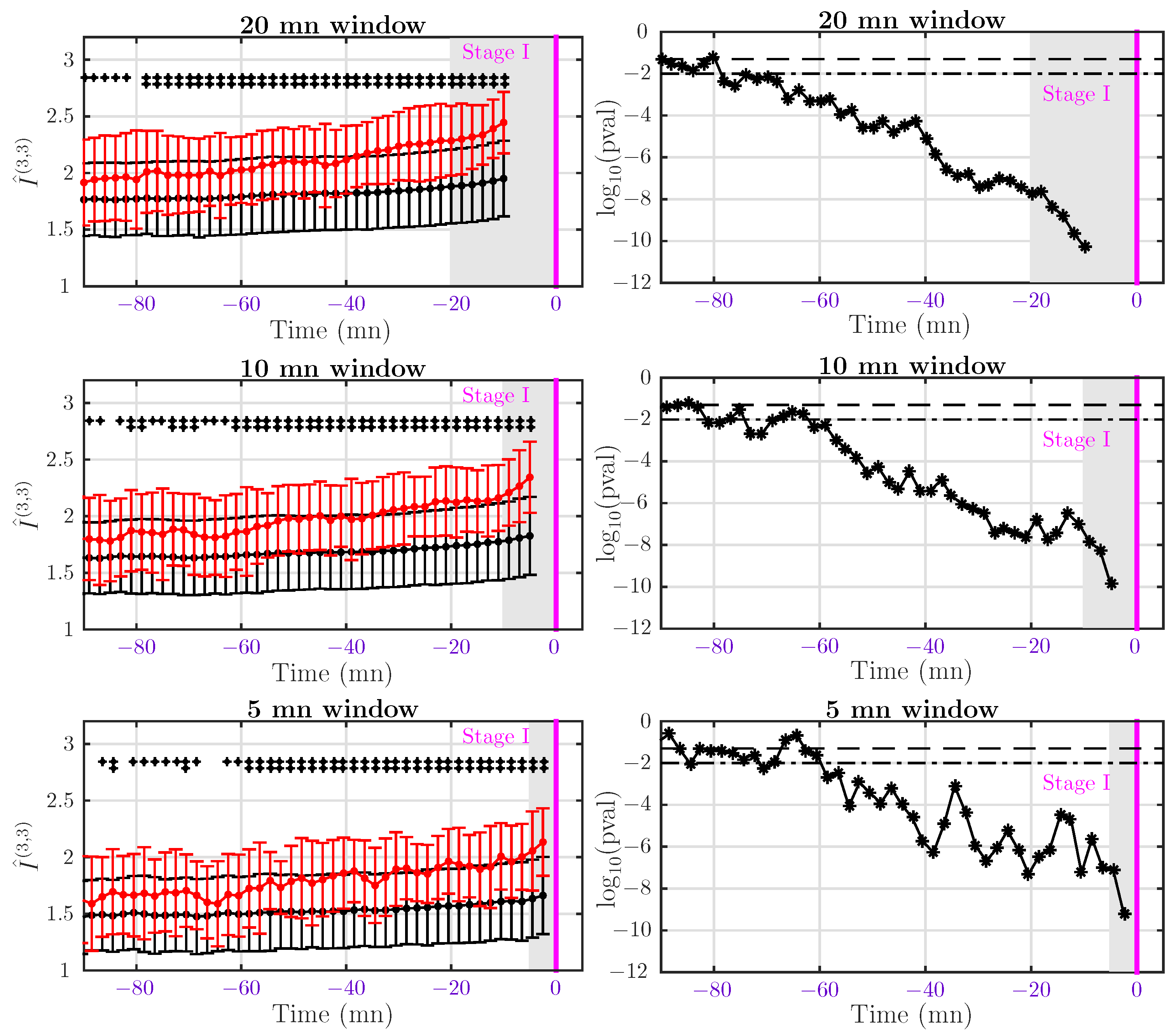
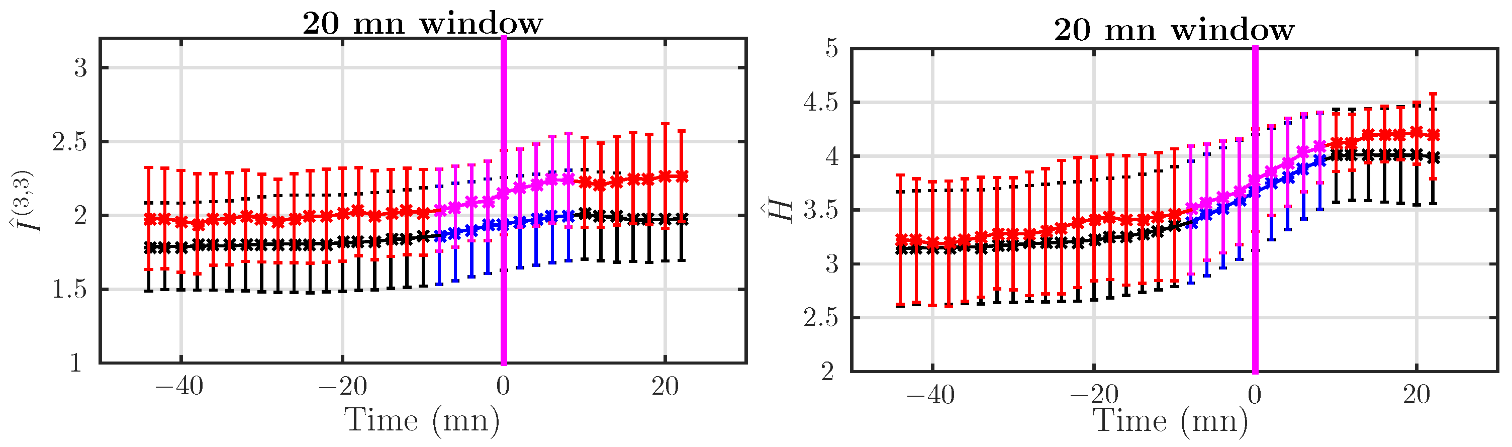
4.4. Dynamical Analysis
4.4.1. Dataset I: Rapid Delivery
4.4.2. Dataset II: Delivery after Pushing More Than 15 mn
5. Discussion, Conclusions and Perspectives
5.1. Acidosis Detection in the First Stage
5.2. Acidosis Detection in Second Stage
5.3. Probing the Dynamics
Acknowledgments
Author Contributions
Conflicts of Interest
References
- Chandraharan, E.; Arulkumaran, S. Prevention of birth asphyxia: Responding appropriately to cardiotocograph (CTG) traces. Best Pract. Res. Clin. Obstet. Gynaecol. 2007, 21, 609–624. [Google Scholar] [CrossRef] [PubMed]
- Ayres-de-Campos, D.; Spong, C.Y.; Chandraharan, E.; The FIGO Intrapartum Fetal Monitoring Expert Consensus Panel. FIGO consensus guidelines on intrapartum fetal monitoring: Cardiotocography. Int. J. Gynaecol. Obstet. 2015, 131, 13–24. [Google Scholar] [CrossRef] [PubMed]
- Rooth, G.; Huch, A.; Huch, R. Guidelines for the Use of Fetal Monitoring. Int. J. Gynaecol. Obstet. 1987, 25, 159–167. [Google Scholar]
- Hruban, L.; Spilka, J.; Chudáček, V.; Janků, P.; Huptych, M.; Burša, M.; Hudec, A.; Kacerovský, M.; Koucký, M.; Procházka, M.; et al. Agreement on intrapartum cardiotocogram recordings between expert obstetricians. J. Eval. Clin. Pract. 2015, 21, 694–702. [Google Scholar] [CrossRef] [PubMed]
- Alfirevic, Z.; Devane, D.; Gyte, G.M. Continuous cardiotocography (CTG) as a form of electronic fetal monitoring (EFM) for fetal assessment during labor. Cochrane Database Syst. Rev. 2006, 3. [Google Scholar] [CrossRef]
- Spilka, J.; Chudáček, V.; Koucký, M.; Lhotská, L.; Huptych, M.; Janků, P.; Georgoulas, G.; Stylios, C. Using nonlinear features for fetal heart rate classification. Biomed. Signal Process. Control 2012, 7, 350–357. [Google Scholar] [CrossRef]
- Haritopoulos, M.; Illanes, A.; Nandi, A. Survey on Cardiotocography Feature Extraction Algorithms for Fetal Welfare Assessment. In XIV Mediterranean Conference on Medical and Biological Engineering and Computing (MEDICON); Kyriacou, E., Christofides, S., Pattichis, C.S., Eds.; Springer International Publishing: Cham, Switzerland, 2016; pp. 1193–1198. [Google Scholar]
- Akselrod, S.; Gordon, D.; Ubel, F.A.; Shannon, D.C.; Berger, A.C.; Cohen, R.J. Power spectrum analysis of heart rate fluctuation: A quantitative probe of beat-to-beat cardiovascular control. Science 1981, 213, 220–222. [Google Scholar] [CrossRef] [PubMed]
- Gonçalves, H.; Rocha, A.P.; de Campos, D.A.; Bernardes, J. Linear and nonlinear fetal heart rate analysis of normal and acidemic fetuses in the minutes preceding delivery. Med. Biol. Eng. Comput. 2006, 44, 847–855. [Google Scholar] [CrossRef] [PubMed]
- Van Laar, J.; Porath, M.; Peters, C.; Oei, S. Spectral analysis of fetal heart rate variability for fetal surveillance: Review of the literature. Acta Obstet. Gynecol. Scand. 2008, 87, 300–306. [Google Scholar] [CrossRef] [PubMed]
- Siira, S.M.; Ojala, T.H.; Vahlberg, T.J.; Rosén, K.G.; Ekholm, E.M. Do spectral bands of fetal heart rate variability associate with concomitant fetal scalp pH? Early Hum. Dev. 2013, 89, 739–742. [Google Scholar] [CrossRef] [PubMed]
- Francis, D.P.; Willson, K.; Georgiadou, P.; Wensel, R.; Davies, L.; Coats, A.; Piepoli, M. Physiological basis of fractal complexity properties of heart rate variability in man. J. Physiol. 2002, 542, 619–629. [Google Scholar] [CrossRef] [PubMed]
- Doret, M.; Helgason, H.; Abry, P.; Gonçalvés, P.; Gharib, C.; Gaucherand, P. Multifractal analysis of fetal heart rate variability in fetuses with and without severe acidosis during labor. Am. J. Perinatol. 2011, 28, 259–266. [Google Scholar] [CrossRef] [PubMed]
- Doret, M.; Spilka, J.; Chudáček, V.; Gonçalves, P.; Abry, P. Fractal Analysis and Hurst Parameter for intrapartum fetal heart rate variability analysis: A versatile alternative to Frequency bands and LF/HF ratio. PLoS ONE 2015, 10, e0136661. [Google Scholar] [CrossRef] [PubMed]
- Echeverria, J.C.; Hayes-Gill, B.R.; Crowe, J.A.; Woolfson, M.S.; Croaker, G.D.H. Detrended fluctuation analysis: A suitable method for studying fetal heart rate variability? Physiol. Meas. 2004, 25, 763–774. [Google Scholar] [CrossRef] [PubMed]
- Chudáček, V.; Anden, J.; Mallat, S.; Abry, P.; Doret, M. Scattering Transform for Intrapartum Fetal Heart Rate Variability Fractal Analysis: A Case-Control Study. IEEE Trans. Biomed. Eng. 2014, 61, 1100–1108. [Google Scholar] [CrossRef] [PubMed]
- Magenes, G.; Signorini, M.G.; Arduini, D. Classification of cardiotocographic records by neural networks. Proc. IEEE-INNS-ENNS Int. Jt. Conf. Neural Netw. 2000, 3, 637–641. [Google Scholar]
- Pincus, S.M.; Viscarello, R.R. Approximate entropy: A regularity measure for fetal heart rate analysis. Obstet. Gynecol. 1992, 79, 249–255. [Google Scholar] [PubMed]
- Pincus, S. Approximate entropy (ApEn) as a complexity measure. Chaos 1995, 5, 110–117. [Google Scholar] [CrossRef] [PubMed]
- Lake, D.E.; Richman, J.S.; Griffin, M.P.; Moorman, J.R. Sample entropy analysis of neonatal heart rate variability. Am. J. Physiol. Regul. Integr. Comp. Physiol. 2002, 283, R789–R797. [Google Scholar] [CrossRef] [PubMed]
- Georgieva, A.; Payne, S.J.; Moulden, M.; Redman, C.W.G. Artificial neural networks applied to fetal monitoring in labor. Neural Comput. Appl. 2013, 22, 85–93. [Google Scholar] [CrossRef]
- Czabanski, R.; Jezewski, J.; Matonia, A.; Jezewski, M. Computerized analysis of fetal heart rate signals as the predictor of neonatal acidemia. Expert Syst. Appl. 2012, 39, 11846–11860. [Google Scholar] [CrossRef]
- Warrick, P.; Hamilton, E.; Precup, D.; Kearney, R. Classification of normal and hypoxic fetuses from systems modeling of intrapartum cardiotocography. IEEE Trans. Biomed. Eng. 2010, 57, 771–779. [Google Scholar] [CrossRef] [PubMed]
- Spilka, J.; Frecon, J.; Leonarduzzi, R.; Pustelnik, N.; Abry, P.; Doret, M. Sparse Support Vector Machine for Intrapartum Fetal Heart Rate Classification. IEEE J. Biomed. Health Inf. 2016, 21, 1–8. [Google Scholar] [CrossRef] [PubMed]
- Dawes, G.; Moulden, M.; Sheil, O.; Redman, C. Approximate entropy, a statistic of regularity, applied to fetal heart rate data before and during labor. Obstet. Gynecol. 1992, 80, 763–768. [Google Scholar] [PubMed]
- Richman, J.S.; Moorman, J.R. Physiological time-series analysis using approximate entropy and sample entropy. Am. J. Physiol. Heart Circ. Physiol. 2000, 278, H2039–H2049. [Google Scholar] [PubMed]
- Grünwald, P.; Vitányistard, P. Kolmogorov complexity and information theory. With an interpretation in terms of questions and answers. J. Log. Lang. Inf. 2003, 12, 497–529. [Google Scholar] [CrossRef]
- Lake, D.E. Renyi entropy measures of heart rate Gaussianity. IEEE Trans. Biomed. Eng. 2006, 53, 21–27. [Google Scholar] [CrossRef] [PubMed]
- Grassberger, P.; Procaccia, I. Estimation of the Kolmogorov-entropy from a Chaotic Signal. Phys. Rev. A 1983, 28, 2591–2593. [Google Scholar] [CrossRef]
- Kozachenko, L.F.; Leonenko, N.N. Sample Estimate of the Entropy of a Random Vector. Probl. Inf. Transm. 1987, 23, 95–101. [Google Scholar]
- Porta, A.; Bari, V.; Bassani, T.; Marchi, A.; Tassin, S.; Canesi, M.; Barbic, F.; Furlan, R. Entropy-based complexity of the cardiovascular control in Parkinson disease: Comparison between binning and k-nearest-neighbor approaches. In Proceedings of the IEEE Engineering in Medicine and Biology Society (EMBC), Osaka, Japan, 3–7 July 2013; pp. 5045–5048. [Google Scholar]
- Spilka, J.; Roux, S.; Garnier, N.; Abry, P.; Goncalves, P.; Doret, M. Nearest-neighbor based wavelet entropy rate measures for intrapartum fetal heart rate variability. In Proceedings of the IEEE Engineering in Medicine and Biology Society (EMBC), Chicago, IL, USA, 26–30 August 2014; pp. 2813–2816. [Google Scholar]
- Xiong, W.; Faes, L.; Ivanov, P.C. Entropy measures, entropy estimators, and their performance in quantifying complex dynamics: Effects of artifacts, nonstationarity, and long-range correlations. Phys. Rev. E 2017, 95, 062114. [Google Scholar] [CrossRef] [PubMed]
- Costa, A.; Ayres-de Campos, D.; Costa, F.; Santos, C.; Bernardes, J. Prediction of neonatal acidemia by computer analysis of fetal heart rate and ST event signals. Am. J. Obstet. Gynecol. 2009, 201, 464.e1–464.e6. [Google Scholar] [CrossRef] [PubMed]
- Georgieva, A.; Papageorghiou, A.T.; Payne, S.J.; Moulden, M.; Redman, C.W.G. Phase-rectified signal averaging for intrapartum electronic fetal heart rate monitoring is related to acidaemia at birth. BJOG 2014, 121, 889–894. [Google Scholar] [CrossRef] [PubMed]
- Spilka, J.; Abry, P.; Goncalves, P.; Doret, M. Impacts of first and second labor stages on Hurst parameter based intrapartum fetal heart rate analysis. In Proceedings of the IEEE Computing in Cardiology Conference (CinC), Cambridge, MA, USA, 7–10 September 2014; pp. 777–780. [Google Scholar]
- Lim, J.; Kwon, J.Y.; Song, J.; Choi, H.; Shin, J.C.; Park, I.Y. Quantitative comparison of entropy analysis of fetal heart rate variability related to the different stages of labor. Early Hum. Dev. 2014, 90, 81–85. [Google Scholar] [CrossRef] [PubMed]
- Spilka, J.; Leonarduzzi, R.; Chudáček, V.; Abry, P.; Doret, M. Fetal Heart Rate Classification: First vs. Second Stage of Labor. In Proceedings of the 8th International Workshop on Biosignal Interpretation, Osaka, Japan, 1–3 November 2016. [Google Scholar]
- Granero-Belinchon, C.; Roux, S.; Garnier, N.; Abry, P.; Doret, M. Mutual information for intrapartum fetal heart rate analysis. In Proceedings of the IEEE Engineering in Medicine and Biology Society (EMBC), Seogwipo, South Korea, 11–15 July 2017. [Google Scholar]
- Costa, M.; Goldberger, A.L.; Peng, C.K. Multiscale entropy analysis of complex physiologic time series. Phys. Rev. Lett. 2002, 89, 068102. [Google Scholar] [CrossRef] [PubMed]
- Doret, M.; Massoud, M.; Constans, A.; Gaucherand, P. Use of peripartum ST analysis of fetal electrocardiogram without blood sampling: A large prospective cohort study. Eur. J. Obstet. Gynecol. Reprod. Biol. 2011, 156, 35–40. [Google Scholar] [CrossRef] [PubMed]
- Takens, F. Detecting strange attractors in turbulence. Dyn. Syst. Turbul. 1981, 4, 366–381. [Google Scholar]
- Shannon, C. A Mathematical Theory of Communication. Bell Syst. Tech. J. 1948, 27, 388–427. [Google Scholar] [CrossRef]
- Rényi, A. On measures of information and entropy. In Proceedings of the Fourth Berkeley Symposium on Mathematical Statistics and Probability, Berkeley, CA, USA, 20 June–30 July 1960; pp. 547–561. [Google Scholar]
- Kullback, S.; Leibler, R. On information and sufficiency. Ann. Math. Stat. 1951, 22, 79–86. [Google Scholar] [CrossRef]
- Gomez, C.; Lizier, J.; Schaum, M.; Wollstadt, P.; Grutzner, C.; Uhlhaas, P.; Freitag, C.; Schlitt, S.; Bolte, S.; Hornero, R.; et al. Reduced predictable information in brain signals in autism spectrum disorder. Front. Neuroinf. 2014, 8. [Google Scholar] [CrossRef] [PubMed]
- Faes, L.; Porta, A.; Nollo, G. Information Decomposition in Bivariate Systems: Theory and Application to Cardiorespiratory Dynamics. Entropy 2015, 17, 277–303. [Google Scholar] [CrossRef]
- Granero-Belinchon, C.; Roux, S.G.; Garnier, N.B. Scaling of information in turbulence. EPL 2016, 115, 58003. [Google Scholar] [CrossRef]
- Eckmann, J.P.; Ruelle, D. Ergodic-Theory of Chaos and Strange Attractors. Rev. Mod. Phys. 1985, 57, 617–656. [Google Scholar] [CrossRef]
- Pincus, S.M. Approximate Entropy as a Measure of System-complexity. Proc. Natl. Acad. Sci. USA 1991, 88, 2297–2301. [Google Scholar] [CrossRef] [PubMed]
- Krstacic, G.; Krstacic, A.; Martinis, M.; Vargovic, E.; Knezevic, A.; Smalcelj, A.; Jembrek-Gostovic, M.; Gamberger, D.; Smuc, T. Non-linear analysis of heart rate variability in patients with coronary heart disease. Comput. Cardiol. 2002, 29, 673–675. [Google Scholar]
- Richman, J.; Moorman, R. Time series analysis using approximate entropy and sample entropy. Biophys. J. 2000, 78, 218A. [Google Scholar]
- Lake, D. Improved entropy rate estimation in physiological data. In Proceedings of the IEEE Engineering in Medicine and Biology Society (EMBC), Boston, MA, USA, 30 August–3 September 2011; pp. 1463–1466. [Google Scholar]
- Jaynes, E.T. Information Theory and Statistical Mechanics. Phys. Rev. 1957, 106, 620–630. [Google Scholar] [CrossRef]
- Singh, H.; Misra, N.; Hnizdo, V.; Fedorowicz, A.; Demchuk, E. Nearest neighbor estimates of entropy. Am. J. Math. Manag. Sci. 2003, 23, 301–321. [Google Scholar] [CrossRef]
- Kraskov, A.; Stogbauer, H.; Grassberger, P. Estimating mutual information. Phys. Rev. E 2004, 69, 066138. [Google Scholar] [CrossRef] [PubMed]
- Gao, W.; Oh, S.; Viswanath, P. Demystifying Fixed k-Nearest Neighbor Information Estimators. In Proceedings of the IEEE Information Theory (ISIT), Aachen, Germany, 25–30 June 2017. [Google Scholar]
- Freeman, R. Problems with intrapartum fetal heart rate monitoring interpretation and patient management. Obstet. Gynecol. 2002, 100, 813–826. [Google Scholar] [PubMed]
- Signorini, M.; Magenes, G.; Cerutti, S.; Arduini, D. Linear and nonlinear parameters for the analysis of fetal heart rate signal from cardiotocographic recordings. IEEE Trans. Biomed. Eng. 2003, 50, 365–374. [Google Scholar] [CrossRef] [PubMed]
- Gonçalves, H.; Henriques-Coelho, T.; Bernardes, J.; Rocha, A.; Nogueira, A.; Leite-Moreira, A. Linear and nonlinear heart-rate analysis in a rat model of acute anoxia. Physiol. Meas. 2008, 29, 1133–1143. [Google Scholar] [CrossRef] [PubMed]


| Dataset I | Dataset II | |||
|---|---|---|---|---|
| AUC | p-Value | AUC | p-Value | |
| ApEn | 0.76 | 4.08 × 10⁻⁶ | 0.61 | 1.33 × 10⁻¹ |
| SampEn | 0.79 | 5.92 × 10⁻⁷ | 0.67 | 2.35 × 10⁻² ⋆ |
| 0.50 | 9.75 × 10⁻¹ | 0.39 | 1.36 × 10⁻¹ | |
| 0.76 | 8.36 × 10⁻⁶ | 0.56 | 4.23 × 10⁻¹ | |
| 0.84 | 2.00 × 10⁻⁹ | 0.68 | 1.69 × 10⁻² ⋆ | |
| SampEn | |||||||
|---|---|---|---|---|---|---|---|
| AUC | p-Value | AUC | p-Value | AUC | p-Value | ||
| Dataset I | 20 mn | 0.79 | 5.92 × 10⁻⁷ | 0.84 | 2.00 × 10⁻⁹ | 0.88 | 5.46 × 10⁻¹¹ |
| 10 mn | 0.76 | 1.22 × 10⁻⁷ | 0.84 | 2.22 × 10⁻⁹ | 0.87 | 1.40 × 10⁻¹⁰ | |
| 5 mn | 0.72 | 1.97 × 10⁻⁷ | 0.83 | 7.47 × 10⁻⁹ | 0.86 | 6.26 × 10⁻¹⁰ | |
| Dataset II | 20 mn | 0.67 | 2.35 × 10⁻² ⋆ | 0.68 | 1.69 × 10⁻² ⋆ | 0.71 | 5.36 × 10⁻³ |
| 10 mn | 0.62 | 1.56 × 10⁻² ⋆ | 0.64 | 5.87 × 10⁻² | 0.68 | 1.66 × 10⁻² ⋆ | |
| 5 mn | 0.62 | 5.16 × 10⁻² | 0.60 | 1.70 × 10⁻¹ | 0.64 | 7.29 × 10⁻² | |
© 2017 by the authors. Licensee MDPI, Basel, Switzerland. This article is an open access article distributed under the terms and conditions of the Creative Commons Attribution (CC BY) license (http://creativecommons.org/licenses/by/4.0/).
Share and Cite
Granero-Belinchon, C.; Roux, S.G.; Abry, P.; Doret, M.; Garnier, N.B. Information Theory to Probe Intrapartum Fetal Heart Rate Dynamics. Entropy 2017, 19, 640. https://doi.org/10.3390/e19120640
Granero-Belinchon C, Roux SG, Abry P, Doret M, Garnier NB. Information Theory to Probe Intrapartum Fetal Heart Rate Dynamics. Entropy. 2017; 19(12):640. https://doi.org/10.3390/e19120640
Chicago/Turabian StyleGranero-Belinchon, Carlos, Stéphane G. Roux, Patrice Abry, Muriel Doret, and Nicolas B. Garnier. 2017. "Information Theory to Probe Intrapartum Fetal Heart Rate Dynamics" Entropy 19, no. 12: 640. https://doi.org/10.3390/e19120640
APA StyleGranero-Belinchon, C., Roux, S. G., Abry, P., Doret, M., & Garnier, N. B. (2017). Information Theory to Probe Intrapartum Fetal Heart Rate Dynamics. Entropy, 19(12), 640. https://doi.org/10.3390/e19120640