Generalized Skew-Normal Negentropy and Its Application to Fish Condition Factor Time Series

Abstract

The problem of measuring the disparity of a particular probability density function from a normal one has been addressed in several recent studies. The most used technique to deal with the problem has been exact expressions using information measures over particular distributions. In this paper, we consider a class of asymmetric distributions with a normal kernel, called Generalized Skew-Normal (GSN) distributions. We measure the degrees of disparity of these distributions from the normal distribution by using exact expressions for the GSN negentropy in terms of cumulants. Specifically, we focus on skew-normal and modified skew-normal distributions. Then, we establish the Kullback–Leibler divergences between each GSN distribution and the normal one in terms of their negentropies to develop hypothesis testing for normality. Finally, we apply this result to condition factor time series of anchovies off northern Chile.

1. Introduction

Recent studies deal with the problem of measuring the disparity of a particular probability density function (pdf) from the normal one [1]. A typical technique to deal with the problem has been exact expressions using information measures over particular distributions. For example, Vidal et al. [2] measure the sensitivity of the skewness parameter using the $L_1$ distance between symmetric and asymmetric distributions. Stehlík [3] proved results on the decomposition of Kullback–Leibler (KL) divergences [4] in the gamma and normal family for divergence between the Maximum Likelihood Estimator (MLE) of the canonical parameter and the canonical parameter of the regular exponential family [5]. Contreras-Reyes and Arellano-Valle [6] considered Jeffrey’s (J) divergence [7] to compare the multivariate Skew-Normal (SN) from the normal distribution, and Gómez-Villegas et al. [8] assessed the effect of kurtosis deviations from normality on conditional distributions, such as the multivariate exponential power family. Main et al. [9] evaluated the local effect of asymmetry deviations from normality using the KL divergence measure of the SN distribution and then compared the local sensitivity with Mardia’s and Malkovich–Afifi’s skewness indexes. They also agree on the use of the SN model to regulate the asymmetry of an empirical distribution because it reflects the deviation in a tractable way. Dette et al. [10] characterizes the “disparity” between the skew-symmetric models and their symmetric counterparts in terms of the total variation distance, which is later used to construct priors. The paper provides additional insights, to those provided in Vidal et al. [2], on the interpretation of this distance and also discusses the usage of the KL divergence among several other distances.

Some recent applications of measuring the disparity of a particular pdf from the normal one using negentropy include those by Gao and Zhang [11] and Wang et al. [12], where the negentropy method has been successfully applied to seismic wavelet estimation. Pires and Ribeiro [13] considered the negentropy to measure the distance of non-Gaussian information from the normal one in independent components, with application to Northern Hemispheric winter monthly variability of a high-dimensional quasi-geostrophic atmospheric model. Furthermore, Pires and Hannachi [14] used a tensorial invariant approximation of the multivariate negentropy in terms of a linear combination of squared coskewness and cokurtosis. Then, the method was applied to global sea surface temperature anomalies, after data anomalies were tested through a non-Gaussian distribution.

In this paper, we develop a procedure, based on KL divergences, to test the significance of the skewness parameter in the Generalized Skew-Normal (GSN) distributions, a flexible class of distributions that includes the SN and normal ones as particular cases. We consider asymptotic expansions of moments and cumulants for the negentropy of two particular cases: the SN and Modified Skew-Normal (MSN) distributions. Given that SN distributions do not accomplish the regularity condition of Fisher Information Matrix (FIM) at $\eta =0$, normality is tested based on the MSN distribution [15]. This allows one to implement an asymptotic normality test for testing the significance of the skewness parameter. Numerical results are studied by: (a) comparing numerical integration methods with proposed asymptotic expansions; (b) comparing the asymptotic test with the likelihood ratio test and the asymptotic normality test given by Arrué et al. [15] ; and (c) applying the proposed test to condition factor time series of anchovy (Engraulis ringens).

This paper is organized as follows: information theoretic measures are described in Section 2. In Section 3, we provide an asymptotic expansion in terms of the corresponding cumulants for the GSN, SN and MSN negentropies. We also express the KL and J divergences among each GSN distribution and the normal one in terms of negentropies (as cumulants’ expansion series) to develop the hypothesis test about the significance of the skewness parameter together with a simulation study (Section 4). A simulation study is given in Section 5. In Section 6, the real data of the condition factor time series of anchovies off northern Chile illustrate the usefulness of the developed methodology. The discussion concludes the paper.

2. Shannon Entropy and Related Measures

The Shannon Entropy (SE) of a random variable Z with pdf f is given by:

$$\begin{array}{c}\hfill H\left(Z\right)=-E\{logf(Z\left)\right\}.\end{array}$$

(1)

The SE of a localization-scale random variable $X=\mu +\sigma Z$ does not depend on $\mu$ and is such that $H\left(X\right)=log\sigma +H\left(Z\right)$ (see, e.g., [16]). The SE could serve to define a measure of disparity from normality, the so-called negentropy [17], which is zero for a Gaussian variable and positive for any distribution. It is defined by:

$$\begin{array}{c}\hfill N\left(Z\right)=H\left(Z_0^{\prime }\right)-H\left(Z\right),\end{array}$$

(2)

where $Z_0^{\prime }$ is a normal random variable with the same mean and variance as those of Z. Equation (2) expresses the negentropy in terms of the standardized version of Z, say $Z^{*}$, as $N\left(Z\right)=H\left(Z_0\right)-H\left(Z^{*}\right)=N\left(Z^{*}\right)$; here, $Z^{*}$ has zero mean and unit variance. Thus, negentropy measures essentially the amount of information that departs from the normal entropy. Furthermore, clearly, the negentropy becomes the KL divergence (see Equation (3) below) between $Z^{*}$ and $Z_0$.

Given that the calculus of negentropy presents a computational challenge, where the integral involves the pdf of Z [16,18], different approximations of negentropy are used, such as cumulants’ expansion series [17,19]. Withers and Nadarajah [19] provided exact and explicit series expansions for the SE and negentropy of a standardized pdf f on $\mathbb{R}$, in terms of cumulants. Yet, they did not perform numerical studies that allow evaluation and comparison with other procedures in some specific families of distributions.

Other measures related to the SE are KL and J divergences. They measure the degree of divergence between the distributions of two random variables $Z_1$ and $Z_2$ with pdfs $f_1$ and $f_2$, respectively. The KL divergence of the pdf for $Z_1$ from the pdf for $Z_2$ is defined as:

$$K(Z_1,Z_2)=E\left[log\left\{\frac{f_1\left(Z_1\right)}{f_2\left(Z_1\right)}\right\}\right].$$

(3)

as indicated in the notation, the expectation is defined with respect to the pdf $f_1$ for $Z_1$. Since in general $K(Z_1,Z_2)$ differs from $K(Z_2,Z_1)$, the J divergence is considered as a symmetric version of the KL divergence, which is defined by:

$$J(Z_1,Z_2)=K(Z_1,Z_2)+K(Z_2,Z_1).$$

(4)

3. Generalized Skew-Normal Distributions

An attractive class of Skew-Symmetric (SS) distributions defined in terms of the pdf appears in Azzalini [20], Azzalini and Capitanio [21] and Gupta et al. [22]:

$$\begin{array}{c}\hfill f(z;\eta )=2f\left(z\right)G\left\{w\right(z;\eta \left)\right\},z\in \mathbb{R},\end{array}$$

(5)

where $\eta \in \mathbb{R}$ represents a skewness/shape parameter, f and G are the respective pdf and cumulative distribution function (cdf) of symmetrical continuous distributions and $w(z;\eta )$ is an odd function of z, with $w(0;\eta )=0$ for any fixed value of $\eta$. Furthermore, we assume that $w(z;{\eta }_0)=0$ for all z and some value ${\eta }_0$ of $\eta$ (typically ${\eta }_0=0$), so that $f(z;{\eta }_0)=f\left(z\right)$, thus recovering symmetry.

The notation $Z\sim SS(\eta ;f,G,w)$ expresses that random variable Z has a distribution with the pdf given by (5). If $f\left(z\right)=\varphi \left(z\right)$ represents the pdf of the standardized normal distribution, denoted by $N(0,1)$, then (5) becomes a family of skew-symmetric distributions generated by the normal kernel, the GSN family. In this case, $Z\sim GSN(\eta ;G,w)$ emerges. An important property of the GSN random variable Z is that all its moments are finite. In particular, it possesses the same even moments of $Z_0\sim N(0,1)$. For instance, $E\left(Z^2\right)=1$, and so, $Var\left(Z\right)=1-{\mu }_z^2$, where ${\mu }_z=E\left(Z\right)$. The most popular GSN distribution is Skew-Normal (SN) [23], for which $w(z;\eta )=\eta z$ and $G\left(z\right)=\mathsf{\Phi }\left(z\right)$ is the cdf of the standardized normal distribution. Therefore, $Z\sim SN\left(\eta \right)$ expresses that Z follows an SN distribution. The location-scale extension of the SS pdf in (5) follows by applying the Jacobian method to the linear random variable $X=\mu +\sigma Z$, where $\mu \in \mathbb{R}$ and $\sigma >0$. In this case, we state that X follows an SS distribution with location parameter $\mu$, scale parameter $\sigma$ and shape/skewness parameter $\eta$ and obtains $X\sim SS(\mu ,{\sigma }^2,\eta ;f,G,w)$. Furthermore, we write $X\sim GSN(\mu ,{\sigma }^2,\eta ;G,w)$ if $f=\varphi$, $X\sim GSN(\mu ,{\sigma }^2,\eta ;G)$ if $f=\varphi$ and $w(z;\eta )=\eta z$; and $X\sim SN(\mu ,{\sigma }^2,\eta )$ if $f=\varphi$, $w(z;\eta )=\eta z$ and $G=\mathsf{\Phi }$.

Two other members of the GSN family that have been studied recently are the Skew-Normal-Cauchy (SNC) distribution [24,25], which follows from (5) by taking $f\left(z\right)=\varphi \left(z\right)$, $w(z;\eta )=\eta z$ and $G\left(z\right)=1/2+(1/\pi )\arctan \left(z\right)$, and the Modified Skew-Normal (MSN) distribution [15], for which $f\left(z\right)=\varphi \left(z\right)$, $w(z;\eta )=\eta z/\sqrt{1+z^2}$ and $G\left(z\right)=\mathsf{\Phi }\left(z\right)$. Nadarajah and Kotz [24] recall that the SNC distribution appears to attain a higher degree of sharpness than the normal distribution, i.e., disparity exists from the common normal distribution produced by the skewness parameter $\eta$. A random variable Z with the SNC or MSN distribution is denoted, respectively, by $Z\sim SNC\left(\eta \right)$ or $Z\sim MSN\left(\eta \right)$ and by $X\sim SNC(\mu ,{\sigma }^2,\eta ;G)$ or $X\sim MSN(\mu ,{\sigma }^2,\eta ;G)$ for their respective location-scale extensions.

We consider the SE for the GSN subclass, i.e., the SE of $Z\sim GSN(\eta ;G,w)$. Thus, assuming a normal kernel in (5), we get the GSN-SE given by:

$$\begin{array}{c}\hfill H\left(Z\right)=H\left(Z_0\right)-E\left(log\left[2G\right\{w(Z;\eta )\left\}\right]\right),\end{array}$$

(6)

where $H\left(Z_0\right)=(1/2)log\left(2\pi e\right)$ is the SE of $Z_0$. It is assumed that a specific skewness value ${\eta }_0$ exists so that $w(z;{\eta }_0)=0$ and so that $G\left\{w(z;{\eta }_0)\right\}=1/2$, thus recovering symmetry at $\eta ={\eta }_0$. Therefore, at $\eta ={\eta }_0$, Z and $Z_0$ have the same distribution and thus the same SE.

Let ${\mu }_z=E\left(Z\right)$ and ${\sigma }_z^2=Var\left(Z\right)$ be the mean and variance of $Z\sim GSN(\eta ;G,w)$, respectively, which must constitute functions of the skewness parameter $\eta$. Since ${\sigma }_z^2=1-{\mu }_z^2$ and $H\left(Z_0^{\prime }\right)=log{\sigma }_z+H\left(Z_0\right)$, we get from (2) that the negentropy of Z becomes:

$$\begin{array}{c}\hfill N\left(Z\right)=\frac{1}{2}log(1-{\mu }_z^2)+E\left(log\left[2G\right\{w(Z;\eta )\left\}\right]\right).\end{array}$$

(7)

Since at $\eta ={\eta }_0$, we have by symmetry ${\mu }_z=0$ and $w(Z;{\eta }_0)=0$, so the negentropy in this case is null, as expected. Clearly, SE and negentropy depend on the choice of the functions $G(·)$ and $w(·;\eta )$. In this paper, we consider both families of GSN distributions for which ${\eta }_0=0$, with $w(z;0)=w(0;\eta )=0$ and $w(-z;\eta )=w(z;-\eta )$, thus following that $-Z\sim GSN(-\eta ;G,w)$ and recovering the normality at $\eta =0$. Examples of this type of functions are $w(z;\eta )=\eta u\left(z\right)$ and $w(z;\eta )=u\left(\eta z\right)$ for some odd function $u\left(z\right)$, with $u\left(0\right)=0$. In this case, recalling that $\eta Z\stackrel{d}{=}\tau Z_{\tau }$, where $Z_{\tau }\sim GSN(\tau ;G,w)$, $\tau =\left|\eta \right|$, and “$\stackrel{d}{=}$” denotes equality in the distribution, we obtain:

$$\begin{array}{c}\hfill E\left(log\left[2G\right\{w(Z;\eta )\left\}\right]\right)=E\left(log\left[2G\left\{w(Z_{\tau };\tau )\right\}\right]\right),\end{array}$$

(8)

thus $H\left(Z\right)=H\left(Z_{\tau }\right)$ and $N\left(Z\right)=N\left(Z_{\tau }\right)$. That is, the entropy and negentropy of $Z\sim SN\left(\eta \right)$ depend on the skewness parameter $\eta$ only through its absolute value $\tau =\left|\eta \right|$.

We have interest in both KL and J divergences for a GSN distribution with respect to the normal distribution. that is, assuming in (3) and (4) that $Z_1=Z\sim GSN(\eta ;G,w)$ and $Z_2=Z_0$. In this case, remembering that $\eta Z\stackrel{d}{=}\tau Z_{\tau }$, where $Z_{\tau }\sim GSN(\tau ;G,w)$ and $\tau =\left|\eta \right|$, we have $K(Z,Z_0)=K(Z_{\tau },Z_0)$ and $K(Z_0,Z)=K(Z_0,Z_{\tau })$, with:

$$K(Z_{\tau },Z_0)=E\left(log\left[2G\left\{w(Z_{\tau };\tau )\right\}\right]\right)\mathrm{and}K(Z_0,Z_{\tau })=-E\left(log\left[2G\left\{w(Z_0;\tau )\right\}\right]\right).$$

(9)

Therefore, $J(Z,Z_0)=J(Z_{\tau },Z_0)$, with:

$$J(Z_{\tau },Z_0)=E\left(log\left[2G\left\{w(Z_{\tau };\tau )\right\}\right]\right)-E\left(log\left[2G\left\{w(Z_0;\tau )\right\}\right]\right).$$

(10)

We also develop asymptotic expansions of the J divergence for the SN and MSN distributions from the normal distribution. To do this, we consider the following preliminary result, the proof of which stems from (9) and (10) by using the Taylor expansion of $\zeta (z;\tau )=log\left[2G\right\{w(z;\tau )\left\}\right]$ at $z=0$ and also because of the facts that (a) all moments of $Z_{\tau }\sim GSN(\tau ;G,w)$ are finite and (b) $Z_{\tau }$ and $Z_0$ contain the same even moments.

Lemma 1.

Consider the composite function $\zeta (z;\tau )=log\left[2G\right\{w(z;\tau )\left\}\right]$, $\tau >0$, by assuming that both functions $G\left(z\right)$ and $w(z;\tau )$ are infinitely differentiable; hence, also $\zeta (z;\tau )$ is infinitely differentiable at $z=0$. If $Z_{\tau }\sim GSN(\tau ;G,u)$, then:

$$\begin{array}{ccc}\hfill K(Z_{\tau },Z_0)& =& \sum _{k=1}^{\infty }\frac{{\zeta }^{\left(k\right)}(0;\tau )}{k!}E\left(Z_{\tau }^k\right),\hfill \\ \hfill J(Z_{\tau },Z_0)& =& \sum _{k=1}^{\infty }\frac{{\zeta }^{(2k-1)}(0;\tau )}{(2k-1)!}E\left(Z_{\tau }^{2k-1}\right),\hfill \end{array}$$

(11)

where ${\zeta }^{\left(k\right)}(z;\tau )$ is the k-th derivative of $\zeta (z;\tau )$. Moreover, from (11), the expressions (6) and (7) for the SE and negentropy of the GSN distributions have the forms:

$$\begin{array}{ccc}\hfill H\left(Z_{\tau }\right)& =& \frac{1}{2}log\left(2\pi e\right)-\sum _{k=1}^{\infty }\frac{{\zeta }^{\left(k\right)}(0;\tau )}{k!}E\left(Z_{\tau }^k\right),\hfill \\ \hfill N\left(Z_{\tau }\right)& =& \frac{1}{2}log(1-{\mu }_{\tau }^2)+\sum _{k=1}^{\infty }\frac{{\zeta }^{\left(k\right)}(0;\tau )}{k!}E\left(Z_{\tau }^k\right),\hfill \end{array}$$

respectively, where ${\mu }_{\tau }=E\left(Z_{\tau }\right)$.

Notice in Lemma 1 that the coefficient ${\zeta }^{\left(k\right)}(0;\tau )$ depends on the derivatives of $G\left(z\right)$ and $w(z;\tau )$ at $z=0$, which change for different GSN distributions. Moreover, since the expansion of $\zeta (z;\tau )$ emerges around $z=0$ by assuming a fixed $\tau$, the approximations may not be reasonable for some values of $\tau$.

3.1. Skew-Normal Distribution

If $Z\sim SN\left(\eta \right)$ or $Z\sim SN(0,1,\eta )$ represents an SN random variable, then its pdf is:

$$\begin{array}{c}\hfill f(z;\eta )=2\varphi \left(z\right)\mathsf{\Phi }\left(\eta z\right),z\in \mathbb{R}.\end{array}$$

Clearly, if $\eta ={\eta }_0=0$, then (12) reduces to the $N(0,1)$-pdf. The SN random variable Z can be conveniently represented as a linear combination of half-normal and normal variables through the following stochastic representation [26]:

$$Z\stackrel{d}{=}\delta |U_0|+\sqrt{1-{\delta }^2}U,$$

(12)

where $\delta =\eta /\sqrt{1+{\eta }^2}$, $U_0$ and U are independent and identically distributed with a unit normal distribution. In particular, since the half-normal random variable $|U_0|$ has mean $b=\sqrt{2/\pi }$ and variance one, it follows from (12) that the mean and variance of $Z_{\tau }$, $\tau =\left|\eta \right|$, are given by:

$$\begin{array}{c}\hfill E\left(Z_{\tau }\right)=b{\delta }_{\tau }\mathrm{and}\mathrm{Var}\left(Z_{\tau }\right)=1-{\left(b{\delta }_{\tau }\right)}^2,\end{array}$$

(13)

where ${\delta }_{\tau }=\tau /\sqrt{1+{\tau }^2}$.

In the SN case, $G\left(z\right)=\mathsf{\Phi }\left(z\right)$ and $w(z;\eta )=\eta z$, which are both infinitely differentiable functions at $z=0$. Consequently, the function $\zeta (z;\tau )={\zeta }_0\left(\tau z\right)=log\left\{2\mathsf{\Phi }\left(\tau z\right)\right\}$ is also infinitely differentiable at $z=0$, thus admitting a Taylor expansion about zero. Therefore, since ${\zeta }^{\left(k\right)}(z;\tau )={\tau }^k{\zeta }_k\left(\tau z\right)$, where ${\zeta }_k\left(x\right)$ is the k-th derivative of ${\zeta }_0\left(x\right)=log\left\{2\mathsf{\Phi }\left(x\right)\right\}$, the expansion (11) in Lemma 1 of $E\left\{\zeta (Z_{\tau };\tau )\right\}=E\left\{{\zeta }_0\left(\tau Z_{\tau }\right)\right\}$, $Z_{\tau }\sim SN\left(\tau \right)$, becomes:

$$E\left\{{\zeta }_0\left(\tau Z_{\tau }\right)\right\}=\sum _{k=1}^{\infty }\frac{{\tau }^k{\kappa }_k{\mu }_k}{k!},$$

(14)

where ${\kappa }_k={\zeta }_k\left(0\right)$ and ${\mu }_k=E\left(Z_{\tau }^k\right)$ (see Appendix A).

In summary, since the even moments of $Z_{\tau }\sim SN\left(\tau \right)$ are also the even moments of $Z_0$, Equation (14) can be rewritten as:

$$\begin{array}{ccc}\hfill E\left\{{\zeta }_0\left(\tau Z_{\tau }\right)\right\}& =& \underset{E\left\{{\zeta }_0\left(\tau Z_0\right)\right\}}{\underbrace{\sum _{k=1}^{\infty }\frac{{\tau }^{2k}{\kappa }_{2k}}{\left(2k\right)!}{\mu }_{2k}}}+\underset{J(Z_{\tau },Z_0)}{\underbrace{\sum _{k=1}^{\infty }\frac{{\tau }^{2k-1}{\kappa }_{2k-1}}{(2k-1)!}{\mu }_{2k-1}}}.\hfill \end{array}$$

Hence, considering also Equation (13), we can compute for the SN case the results for the KL and J divergences, SE and negentropy given in Lemma 1 using the following Proposition 1.

Proposition 1.

Let $Z_{\tau }\sim SN\left(\tau \right)$ and $Z_0\sim N(0,1)$. Then:

$$\begin{array}{ccc}\hfill K(Z_{\tau },Z_0)& =& \sum _{k=1}^{\infty }\frac{{\tau }^k{\kappa }_k{\mu }_k}{k!},\hfill \\ \hfill J(Z_{\tau },Z_0)& =& b\sum _{k=1}^{\infty }\frac{{\kappa }_{2k-1}{\delta }_{\tau }^{2k-1}}{(2k-1)!}\sum _{m=1}^k{a}_k\left(m\right){\tau }^{2m-1},\hfill \\ \hfill H\left(Z_{\tau }\right)& =& \frac{1}{2}log\left(2\pi e\right)-K(Z_{\tau },Z_0),\hfill \\ \hfill N\left(Z_{\tau }\right)& =& \frac{1}{2}log\{1-{\left(b{\delta }_{\tau }\right)}^2\}+K(Z_{\tau },Z_0),\hfill \end{array}$$

(15)

where the coefficients $a_k\left(m\right)$, $k=1,2,\dots$, are given in the Appendix A.

To gain a more complete analysis of the behavior of these series, we need appropriate forms for the calculation of the coefficients ${\kappa }_k={\zeta }_k\left(0\right)$, $k=1,2,\dots$ (see Appendix A).

3.2. Modified Skew-Normal Distribution

The pdf for a random variable Z with MSN distribution, denoted by $Z\sim MSN\left(\eta \right)$, is given by:

$$\begin{array}{c}\hfill f\left(z\right)=2\varphi \left(z\right)\mathsf{\Phi }\left\{\eta u\left(z\right)\right\},z\in \mathbb{R},\end{array}$$

where $u\left(z\right)=z/\sqrt{1+z^2}$. Similarly to the SN case, the MSN random variable $Z_{\tau }\sim MSN\left(\tau \right)$, $\tau =\left|\eta \right|$, has even moments equal to the corresponding even moments of the standardized normal random variable $Z_0$ [15], i.e., ${\mu }_{2k}=(2k-1)!!=\left(2k\right)!/(2^{k}k!)$ (for odd moments ${\mu }_{2k-1}\left(\tau \right)$, $k=1,2,\dots$, see Appendix A).

In the MSN case, $G\left(w\right)=\mathsf{\Phi }\left(w\right)$ and $w(z;\tau )=\tau u\left(z\right)=\tau z/\sqrt{1+z^2}$, both of which are infinitely differentiable at $z=0$. Thus, in Lemma 1, we have $\zeta (z;\tau )={\zeta }_0\left\{\tau u\left(z\right)\right\}$, where ${\zeta }_0\left(x\right)=log\left\{2\mathsf{\Phi }\left(x\right)\right\}$ is also infinitely differentiable at $z=0$. Thus, the series expansion of $E\left\{\zeta (Z_{\tau };\tau )\right\}=E\left[{\zeta }_0\left\{\tau u\left(Z_{\tau }\right)\right\}\right]$, $Z_{\tau }\sim MSN\left(\tau \right)$, can be obtained from (11) for which we need the derivatives of the composite function ${\zeta }_0\left\{\tau u\left(z\right)\right\}=log\left[2\mathsf{\Phi }\left\{\tau u\left(z\right)\right\}\right]$. Another way to obtain these derivatives is to define random variable $Z_{\tau }^{*}=u\left(Z_{\tau }\right)=Z_{\tau }/\sqrt{1+Z_{\tau }^2}$ and using (14) with $Z_{\tau }$ and ${\mu }_k=E\left(Z_{\tau }\right)$ replaced by $Z_{\tau }^{*}$ and ${\mu }_k^{*}=E\{{\left(Z_{\tau }^{*}\right)}^k\}$, respectively. Thus, we obtain the series expansion:

$$E\left\{{\zeta }_0\left(\tau Z_{\tau }^{*}\right)\right\}=\sum _{k=1}^{\infty }\frac{{\tau }^k{\kappa }_k}{k!}{\mu }_k^{*}.$$

From Lemma 1, the KL and J divergences, SE and negentropy for the MSN case can be computed using the following Proposition 2.

Proposition 2.

Let $Z_{\tau }\sim MSN\left(\tau \right)$ and $Z_0\sim N(0,1)$. Then:

$$\begin{array}{ccc}\hfill K(Z_{\tau },Z_0)& =& \sum _{k=1}^{\infty }\frac{{\tau }^k{\kappa }_k}{k!}{\mu }_k^{*},\hfill \\ \hfill J(Z_{\tau },Z_0)& =& \sum _{k=1}^{\infty }\frac{{\tau }^{2k-1}{\kappa }_{2k-1}}{(2k-1)!}{\mu }_{2k-1}^{*},\hfill \\ \hfill H\left(Z_{\tau }\right)& =& \frac{1}{2}log\left(2\pi e\right)-K(Z_{\tau },Z_0),\hfill \\ \hfill N\left(Z_{\tau }\right)& =& \frac{1}{2}log(1-{\left[b\{2{\xi }_1\left(\tau \right)-1\}\right]}^2)+K(Z_{\tau },Z_0).\hfill \end{array}$$

(16)

In order to compute the quantities given by Proposition 2, we need to calculate the new moments ${\mu }_k^{*}=E\{{\left(Z_{\tau }^{*}\right)}^k\}$, $k=1,2,...$. Since $Z_{\tau }^{*}=Z_{\tau }/\sqrt{1+Z_{\tau }^2}$ is a random variable limited to the interval $(-1,1)$, all its moments are finite. In particular, $Z_{\tau }^{*}$ clearly has the same even moments as $Z_0^{*}=Z_0/\sqrt{1+Z_0^2}$ Moreover, from the Jacobian method, the pdf of $Z_{\tau }^{*}$ becomes:

$$\begin{array}{c}\hfill f^{*}\left(u\right)=\frac{2}{{(1-u^2)}^{3/2}}\varphi \left(\frac{u}{\sqrt{1-u^2}}\right)\mathsf{\Phi }\left(\tau u\right),u\in (-1,1).\end{array}$$

Hence, the k-th moment of $Z_{\tau }^{*}$ is:

$${\mu }_k^{*}={\int }_{-1}^1{u}^k{f}^{*}\left(u\right)du,k=1,2,\dots ,$$

which must be computed numerically.

3.3. J Divergence between SN and MSN Distributions

In the previous sections, SN and MSN distributions were compared with the normal distribution by means of the J divergence measure. As a byproduct, we were also computing the J divergence between the SN and MSN distributions, both with the same skewness parameter. This allows measuring the distance between these distributions with different $w(z;\eta )$’s. For this, we consider in Equation (4) that $Z_1\sim SN\left(\tau \right)$ and $Z_2\sim MSN\left(\tau \right)$ and define the random variables $Z_i^{*}=Z_i/\sqrt{1+Z_i^2}$ for $i=0,1,2$, where $Z_0\sim N(0,1)$. Let ${\mu }_{i,k}=E\left(Z_i^k\right)$ and ${\mu }_{i,k}^{*}=E\{{\left(Z_i^{*}\right)}^k\}$, $i=0,1,2$. Recall that ${\mu }_{i,2k}={\mu }_{0,2k}$ and ${\mu }_{i,2k}^{*}={\mu }_{0,2k}^{*}$ for all $k=1,2,\dots$. Thus, using (4) and then the Taylor expansion of ${\zeta }_0\left(x\right)=log\left\{\mathsf{\Phi }\left(x\right)\right\}$ around $x=0$, Proposition 3 is obtained:

Proposition 3.

Let $Z_0\sim N(0,1)$, $Z_1\sim SN\left(\tau \right)$ and $Z_2\sim MSN\left(\tau \right)$. Define the random variables $Z_i^{*}=Z_i/\sqrt{1+Z_i^2}$, $i=1,2$. Then:

$$\begin{array}{ccc}\hfill J(Z_1,Z_2)& =& E\left\{{\zeta }_0\left(\tau Z_1\right)\right\}-E\left\{{\zeta }_0\left(\tau Z_1^{*}\right)\right\}+E\left\{{\zeta }_0\left(\tau Z_2^{*}\right)\right\}-E\left\{{\zeta }_0\left(\tau Z_2\right)\right\}\hfill \\ & =& J(Z_1,Z_0)-J(Z_1^{*},Z_0)+J(Z_2^{*},Z_0)-J(Z_2,Z_0),\hfill \end{array}$$

where as before:

$$\begin{array}{ccc}\hfill J(Z_i,Z_0)& =& \sum _{k=1}^{\infty }{\tau }^{2k-1}\frac{{\mu }_{i,2k-1}{\kappa }_{2k-1}}{(2k-1)!},\hfill \\ \hfill J(Z_i^{*},Z_0)& =& \sum _{k=1}^{\infty }{\tau }^{2k-1}\frac{{\mu }_{i,2k-1}^{*}{\kappa }_{2k-1}}{(2k-1)!},i=1,2.\hfill \end{array}$$

Proposition 3 indicates that J divergence between SN and MSN distributions is decomposed to the divergences of the normal distribution with each of these distributions, which depends only on their odd moments and cumulants.

4. Asymptotic Tests

Let $f(x;\mathit{\theta })$, $x\in \mathcal{X}$, $\mathit{\theta }\in \mathsf{\Theta }$, be the pdf of a regular parametric class of distributions, i.e., for which the sample space $\mathcal{X}$ does not depend on $\mathit{\theta }$, the parametric space $\mathsf{\Theta }$ is an open subset of ${\mathbb{R}}^p$, and the regularity conditions (i)–(iii) stated in Salicrú et al. [27] are satisfied. As in Salicrú et al. [27], we denote the KL divergence between $f(x;\mathit{\theta })$ and $f(x;{\mathit{\theta }}^{\prime })$, $\mathit{\theta },{\mathit{\theta }}^{\prime }\in \mathsf{\Theta }$, by:

$$K(\mathit{\theta },{\mathit{\theta }}^{\prime })={\int }_{\mathcal{X}}f(x;\mathit{\theta })log\left\{\frac{f(x;\mathit{\theta })}{f(x;{\mathit{\theta }}^{\prime })}\right\}dx.$$

Consider the partition $\mathit{\theta }=({\mathit{\theta }}_1,{\mathit{\theta }}_2)$, where ${\mathit{\theta }}_1\in {\mathsf{\Theta }}_1\subset {\mathbb{R}}^r$ and ${\mathit{\theta }}_2\in {\mathsf{\Theta }}_2=\mathsf{\Theta }\cap {\mathsf{\Theta }}_1^c\subset {\mathbb{R}}^{p-r}$. Let ${\mathit{\theta }}^{\prime }=({\mathit{\theta }}_1,{\mathit{\theta }}_2^0)$ and consider the null hypothesis $H_0:{\mathit{\theta }}_2={\mathit{\theta }}_2^0$ for a known ${\mathit{\theta }}_2^0\in \mathsf{\Theta }\cap {\mathsf{\Theta }}_1^c$. Let $\widehat{\mathit{\theta }}=({\widehat{\mathit{\theta }}}_1,{\widehat{\mathit{\theta }}}_2)$ and $\widehat{{\mathit{\theta }}^{\prime }}=({\widehat{\mathit{\theta }}}_1,{\mathit{\theta }}_2^0)$ be the (unrestricted) MLE of $\mathit{\theta }$ and ${\mathit{\theta }}^{\prime }$, respectively, both based on a random sample of size n from X with pdf $f(x;\mathit{\theta })$. Under these conditions, we have from Part (b) of Theorem 2 presented in Salicrú et al. [27] that:

$$\begin{array}{c}\hfill 2nK(\widehat{\mathit{\theta }},\widehat{{\mathit{\theta }}^{\prime }})=2n{\int }_{\mathcal{X}}f(x;\widehat{\mathit{\theta }})log\left\{\frac{f(x;\widehat{\mathit{\theta }})}{f(x;\widehat{{\mathit{\theta }}^{\prime }})}\right\}dx\underset{n\to \infty }{\stackrel{d}{⟶}}{\chi }_{p-r}^2,\forall \mathit{\theta }\in \mathsf{\Theta },\end{array}$$

(17)

where “$\stackrel{d}{⟶}$” denotes convergence in distribution and ${\chi }_s^2$ denotes the chi-squared distribution function with s degrees of freedom. From (17), the above null hypothesis can be tested by the statistic $2nK(\widehat{\mathit{\theta }},\widehat{{\mathit{\theta }}^{\prime }})$, which is asymptotically chi-squared distributed with $p-r$ degrees of freedom. Specifically, for large values of n, if we observe $K(\widehat{\mathit{\theta }},\widehat{{\mathit{\theta }}^{\prime }})=K_0$, then $H_0$ is rejected at level $\alpha$ if $P({\chi }_{p-r}^2>2n{K}_0)\le \alpha$.

4.1. One-Sample Case: Test for Normality

The result in (17) can be applied for example to construct a normality test from the KL divergence between a regular GSN distribution and the normal distribution. Specifically, consider a random sample $X_1,\dots ,X_n$ from $X\sim GSN(\mu ,{\sigma }^2,\eta ,G,w)$ and the null hypothesis $H_0:\eta ={\eta }_0$ under which $G\left\{w(z;{\eta }_0)\right\}=G\left(0\right)=1/2$; thus, the GSN random variable X becomes a $N(\mu ,{\sigma }^2)$ random variable. Let $\widehat{\mathit{\theta }}=(\widehat{\mu },\widehat{{\sigma }^2},\widehat{\eta })$ be the MLE of $\mathit{\theta }=(\mu ,{\sigma }^2,\eta )$ and $\widehat{{\mathit{\theta }}^{\prime }}=(\widehat{\mu },\widehat{{\sigma }^2},{\eta }_0)$. Therefore, under $H_0:\eta ={\eta }_0$, we have:

$$2nK(\widehat{\mathit{\theta }},\widehat{{\mathit{\theta }}^{\prime }})=2nK(Z_{\widehat{\tau }},Z_0)\underset{n\to \infty }{\stackrel{d}{⟶}}{\chi }_1^2,$$

(18)

where $K(Z_{\widehat{\tau }},Z_0)$ is the MLE of $K(Z_{\tau },Z_0)$, which is defined in Equation (11) of Lemma 1 and depends only on $\widehat{\tau }=\left|\widehat{\eta }\right|$. As stated in the Introduction, normality is typically obtained from the GSN class at ${\eta }_0=0$ or equivalently ${\tau }_0=\left|{\eta }_0\right|=0$.

Azzalini [20], Arellano-Valle and Azzalini [28] and Azzalini and Capitanio [23] recall the singularity of SN FIM at $\eta =0$, preventing the asymptotic distribution of the above statistic tests. As suggested by Azzalini [20], a solution to recover the non-singularity of the information matrix under the symmetry hypothesis comes from the use of the so-called centered parametrization defined in terms of the mean, variance and the skewness parameters of the SN distribution (see also [28,29]). Otherwise, the FIM of the MSN model is non-singular at $\eta =0$ [15]. Thus, this model satisfies all the standard regularity conditions of Salicrú et al. [27], leading to consistence and asymptotic normality of the MLEs under the null hypothesis of normality. Therefore, the MSN model serves to test the null hypothesis of normality using (18). Hence, the symmetry null hypothesis $H_0:\tau =0$ is rejected at level $\alpha$ if $P({\chi }_1^2>2n{K}_0)\le \alpha$, with $K_0=K(Z_{\widehat{\tau }},Z_0)$.

4.2. Two-Sample Case

Consider two independent samples of sizes $n_1$ and $n_2$ from $X_1$ and $X_2$, respectively; where $\mathit{\theta },{\mathit{\theta }}^{\prime }\in \mathsf{\Theta }\subset {\mathbb{R}}^p$, and $X_1$ and $X_2$ have pdf’s $f(x;{\mathit{\theta }}_1)$ and $f(x;{\mathit{\theta }}_2)$, respectively. Suppose partition ${\mathit{\theta }}_i=({\mathit{\theta }}_{i1},{\mathit{\theta }}_{i2})$, $i=1,2$, and assume ${\mathit{\theta }}_{21}={\mathit{\theta }}_{11}\in {\mathsf{\Theta }}_1\subset {\mathbb{R}}^r$, so that ${\mathit{\theta }}_{i2}\in \mathsf{\Theta }\cap {\mathsf{\Theta }}_1^c\subset {\mathbb{R}}^{p-r}$, $i=1,2$. Let ${\widehat{\mathit{\theta }}}_i=({\widehat{\mathit{\theta }}}_{11},{\widehat{\mathit{\theta }}}_{i2})$ be the MLE of ${\mathit{\theta }}_i=({\mathit{\theta }}_{11},{\mathit{\theta }}_{i2})$, $i=1,2$, which correspond to the MLE of the full model parameters $({\mathit{\theta }}_1,{\mathit{\theta }}_2)$ under null hypothesis $H_0:{\mathit{\theta }}_{21}={\mathit{\theta }}_{11}$. Thus, Part (b) of Corollary 1 in Salicrú et al. [27] establishes that if the null hypothesis $H_0:{\mathit{\theta }}_{22}={\mathit{\theta }}_{12}$ holds and $\frac{n_1}{n_1+n_2}\underset{n_1,n_2\to \infty }{⟶}\lambda$, with $0<\lambda <1$, then:

$$\begin{array}{c}\hfill \frac{2n_1{n}_2}{n_1+n_2}K({\widehat{\mathit{\theta }}}_1,{\widehat{\mathit{\theta }}}_2)=\frac{2n_1{n}_2}{n_1+n_2}{\int }_{-\infty }^{\infty }f(x;{\widehat{\mathit{\theta }}}_1)log\left\{\frac{f(x;{\widehat{\mathit{\theta }}}_1)}{f(x;{\widehat{\mathit{\theta }}}_2)}\right\}dx\underset{n_1,n_2\to \infty }{\stackrel{d}{⟶}}{\chi }_{p-r}^2.\end{array}$$

(19)

Thus, a test of level $\alpha$ for the above homogeneity null hypothesis consists of rejecting $H_0$ if:

$$\frac{2n_1{n}_2}{n_1+n_2}K({\widehat{\mathit{\theta }}}_1,{\widehat{\mathit{\theta }}}_2)>{\chi }_{p-r,1-\alpha }^2,$$

where ${\chi }_{p-r,\alpha }^2$ is the $\alpha$-th percentile of the ${\chi }_{p-r}^2$-distribution.

Contreras-Reyes and Arellano-Valle [6] considered the result of Kupperman [30] to develop an asymptotic test of complete homogeneity in terms of the J divergence between two SN distributions. The SN distribution satisfies all the aforementioned regularity conditions when skewness parameter $\eta \ne 0$. Thus, considering this condition, we can also apply (17) and (19) to obtain, respectively, asymptotic tests with one or two samples of other hypotheses not covered by Kupperman’s test.

5. Simulations

In this section, we study the behavior of the series expansions of the SE and negentropy for the SN and MSN distributions. In both cases, we compare the SE and negentropies obtained from their series expansions with their corresponding “exact” versions computed from the Quadpack numerical integration method of Piessens et al. [31]. More precisely, the “exact” expected values $E\left\{{\zeta }_0\left(\tau Z_{\tau }\right)\right\}$ and $E\left\{{\zeta }_0\left(\tau Z_{\tau }^{*}\right)\right\}$ are computed using the Quadpack method as in Arellano-Valle et al. [16], Contreras-Reyes and Arellano-Valle [6] or Contreras-Reyes [18]. From the series expansions, the SE and negentropies were carried out for $k=12$ as in Withers and Nadarajah [19]. However, they tend to converge for $k=4$ as in the Gram–Charlier and Edgeworth expansion methods (see, e.g., Hyvärinen et al. [17] and Stehlík et al. [1], respectively). All proposed methods are implemented with R software [32].

From Figure 1, we observe that the approximations by series expansions are better in the MSN case (Panels C and D) than in the SN case (Panels A and B). Furthermore, that series expansion approximations are quite exact for small to moderate values of the skewness parameter $\tau$; more specifically, for $0\le \tau \le 2$ in the SN case, and $0\le \tau \le 4$ in the MSN case. Additionally, Panels A and C show that the SE decreases as $\tau$ increases, while Panels B and D indicate that the negentropy increases with $\tau$. Finally, as expected in both GSN models, the SE is less than or equal to the SE of the normal model, namely $H\left(Z_0\right)\approx 1.418$ [6,33].

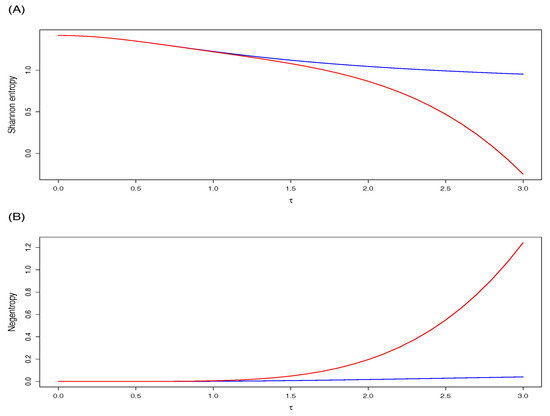
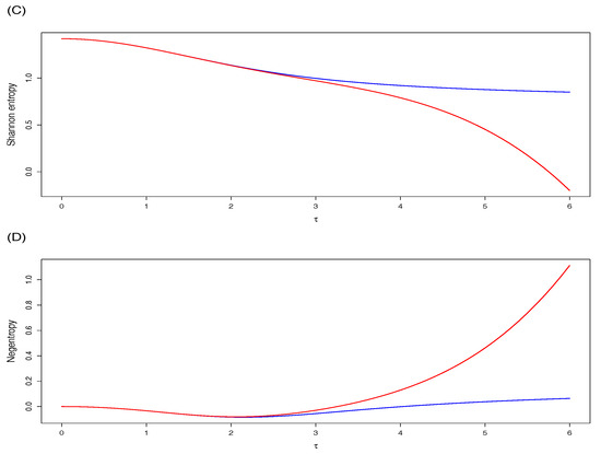
Figure 1. Shannon entropy and negentropy for the (A,B) Skew-Normal (SN) and (C,D) Modified Skew-Normal (MSN) cases. The blue and red lines correspond to numerical integration and cumulant expansion series methods, respectively.

Panel A of Figure 2 shows, respectively, the behavior of the KL divergences of the SN and MSN distributions from the normal one obtained from the expansions in series given in Equations (15) and (16). As in Figure 1, the KL divergence between the SN and normal distributions increases smoothly for values of $\tau \in [0,2]$, but rises sharply for $\tau >2$. Meanwhile, the increase in KL divergence between the MSN and normal distributions seems more stable, at least for $\tau \in [0,5]$. Crucially, for $\tau =\left|\eta \right|\ge 2$, the SN model is close to its maximum level of asymmetry, while the MSN model does it for $\tau =\left|\eta \right|\ge 5$ (see [15] (Figure 2)).

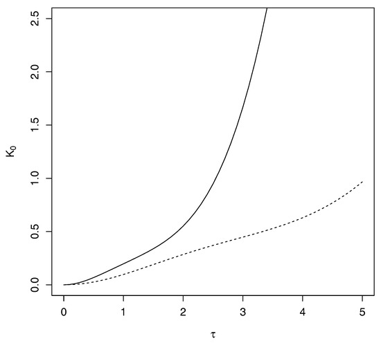
Figure 2. Kullback-Leibler (KL) divergence, $K_0=K(Z_{\tau },Z_0)$, between SN and normal (solid line) and MSN and normal (dotted line).

Table 1 presents the observed power of the asymptotic test of normality obtained from Equation (18) in Section 4.1, for different sample sizes and values of the skewness parameter. All these results were obtained from 2000 simulations for a nominal level of 5%. In each simulation, the MLE of $Z\sim MSN\left(\eta \right)$ was obtained by maximizing the log-likelihood function:

$$\begin{array}{c}\hfill \ell \left(\eta \right)=\frac{n}{2}log\left(2\pi \right)-\frac{1}{2}\sum _{i=1}^n{z}_i^2+\sum _{i=1}^{n}log{\zeta }_0\left\{\eta u\left(z_i\right)\right\},\end{array}$$

(20)

for shape parameter $\eta$ and a random sample of size n from Z [15]. Table 1 shows that the proposed test is considerably conservative since the observed rate of incorrect rejections of the normality hypothesis is always lower than the nominal level. The proposed test is also considerably more powerful in large samples ($n\ge 300$) and values of the skewness parameter far from zero ($\left|\eta \right|\ge 1.2$). As expected, the power of the test increases with sample size, particularly for small values of the skewness parameter (close to normality), given that statistic $2n{K}_0$ depends on n despite $K_0$ being small (Figure 2).

Table 1. Observed power (both in %) of the proposed normality test using the maximum likelihood estimator (MLE) of the MSN model from 2000 simulations for the nominal level of 5% and various values of shape parameter $\eta$ and sample size n.

n/$\mathit{\eta }$	0	0.1	0.2	0.3	0.4	0.8	1.2	1.6	2
50	97.55	37.02	39.45	37.39	37.60	40.07	40.82	48.37	51.29
100	97.65	46.15	45.90	47.90	46.05	50.05	56.10	66.20	75.49
200	98.05	54.25	54.30	53.65	54.50	58.80	70.55	85.20	93.25
300	98.30	57.30	57.70	58.00	58.65	62.00	77.05	92.65	98.25
400	98.55	57.20	57.65	57.15	57.50	64.10	83.95	95.80	99.65
500	98.70	58.55	59.40	59.95	58.45	66.70	86.95	97.45	99.75

Now, we compare the proposed asymptotic test with two additional tests considered by Arrué et al. [15] for null hypothesis $H_0:\eta ={\eta }_0$ versus $H_1:\eta \ne {\eta }_0$: the Likelihood Radio Test (LRT) (see Appendix A) and the asymptotic normality-based test. Since the regularity condition on MSN’s FIM at $\eta =0$ is satisfied, the authors proposed a distributional normal theory for testing $H_0$, i.e., based on asymptotic normality of MLE given by $\sqrt{n}(\widehat{\theta }-{\theta }_0)\stackrel{d}{⟶}{N}_3(0,i_{MSN}^{-1}\left({\theta }_0\right))$, as $n\to \infty$, where $\widehat{\theta }={(\widehat{\mu },{\widehat{\sigma }}^2,\widehat{\eta })}^{\top }$ is the MLE of $\theta ={(\mu ,{\sigma }^2,\eta )}^{\top }$, ${\theta }_0={(\mu ,{\sigma }^2,0)}^{\top }$ and $i_{MSN}^{-1}\left({\theta }_0\right)$ is the inverse FIM component related to ${\theta }_0$. For asymptotic normality and LRT, they conclude that $H_0$ is rejected for large values of $\widehat{\tau }=\left|\widehat{\eta }\right|$, and for large values of n, the coverage rate increases when $\widehat{\eta }$ exists ($H_0$ is rejected) (see [15] (Tables 3–5)). Analogously, in Table 6 of Arrué et al. [15], the coverage rate increase when $\widehat{\eta }$ exists for large values of n.

6. Application to Condition Factor Time Series

To apply our results to a real-world problem, we considered the Condition Factor (CF) index [34], which serves as an important indicator of the fatness condition of fish [18]. The CF index,

$$CF=\frac{W}{\widehat{W}}(100\%),$$

of an individual of length L is computed in terms of the observed weight $W=W\left(L\right)$ and an estimation $\widehat{W}=\widehat{W}\left(L\right)$ obtained from the morphometric relationships of the expected weight $E\left(W\right)$ at length L. Then, the CF index is interpretable as food deficit (<100%) and abundance (>100%) conditions. The expected length-weight relationship is described through the non-linear relationship:

$$E\left(W\right)=\alpha L^{\beta },$$

(21)

where $\alpha$ is the theoretical weight at length zero and $\beta$ is the weight growth rate [35]. According to (21), $\widehat{W}$ is computed as $\widehat{W}=\widehat{\alpha }{L}^{\widehat{\beta }}$, where $\widehat{\alpha }$ and $\widehat{\beta }$ are obtained by fitting the non-linear regression induced by (21) to the length-weight data obtained from a sample of the species under study.

The CF index can be mainly affected by environmental factors such as El Niño (cold events) or La Niña (warm events). These effects are conductors of threshold biological processes due to the limitation of food. For these reasons, Contreras-Reyes [18] considered a threshold autoregressive model based on the stochastic representation (12) to model CF time series. That is, by assuming an SN distribution with skewness parameter $\eta$ for the CF index [20], the condition $\left|\delta \right|<1$ ensures the weak stationarity of the process. Additionally, when $\eta$ is positive, CF values fall below 100% (food deficit). Otherwise, CF values are greater than 100% (food abundance).

We applied hypothesis testing developed in Section 4 to monthly CF time series associated with anchovy from Chile’s northern coast during the period 1990–2010, which were classified by length and sex, for length classes 12,...,18 cm and ALL (all length classes). Therefore, the sample size of each classification depends on the availability of the routine biological sampling program (see more details in [18]). CF were previously standardized, since the shape parameter $\eta$ is not affected by a linear transformation of the CF [23]. Table 2 shows the $\widehat{\eta }$’s assuming an SN and MSN distribution based on the MLE method of Azzalini [36] and Arrué et al. [15], respectively. For MSN, we considered the log-likelihood function of Equation (20). In both models, negative and positive values of $\widehat{\eta }$ correspond to asymmetry to the right and left, respectively (see Contreras-Reyes [18] (Figure 5)). This means that CF of the above-mentioned classes are affected by extreme events. As expected, we find generally that for low values of the empirical skewness index, the shape parameter of both distributions is close to zero.

Table 2. Shape parameter estimates ($\widehat{\eta }$) of SN (reported in [18]) and MSN models for each sex and length class L, together with its respective standard deviations (s.d). Sample size (n), empirical skewness ($\sqrt{{\widehat{b}}_1}$) and kurtosis (${\widehat{b}}_2$), as well as the log-likelihood function $\ell \left(\widehat{\eta }\right)$ for each model fit are also reported.

Sex	L	n	$\sqrt{{\widehat{\mathit{b}}}_1}$	${\widehat{\mathit{b}}}_2$	SN			MSN
					$\widehat{\mathit{\eta }}$	s.d	$\mathit{\ell }\left(\widehat{\mathit{\eta }}\right)$	$\widehat{\mathit{\eta }}$	s.d	$\mathit{\ell }\left(\widehat{\mathit{\eta }}\right)$
Male	12	213	−0.220	3.723	−1.065	0.147	−301.066	−1.717	0.662	−235.783
	13	238	0.658	5.120	1.778	0.134	−332.638	2.617	0.447	−359.291
	14	260	−0.147	2.885	−1.086	0.166	−367.935	0.459	0.542	−342.881
	15	261	−0.030	2.755	−0.442	0.150	−369.834	0.065	0.386	450.489
	16	261	0.307	3.138	1.616	0.149	−367.542	2.565	0.415	−354.073
	17	221	−3.461	27.958	−3.092	0.080	−285.125	−3.597	0.524	−312.701
	18	180	0.264	3.001	1.368	0.201	−253.988	2.821	0.643	−269.193
	All	262	0.068	2.687	0.721	0.178	−371.192	−0.287	0.517	−131.335
Female	12	198	0.041	2.738	0.552	0.196	−280.434	−0.142	0.386	−209.551
	13	228	0.917	6.103	2.267	0.128	−315.305	3.101	0.524	−326.665
	14	260	0.190	2.907	1.242	0.157	−367.555	1.459	0.867	−331.373
	15	260	0.076	2.672	0.728	0.174	−368.344	−0.189	0.383	−425.212
	16	261	0.349	3.091	1.702	0.155	−367.160	2.631	0.475	−346.705
	17	246	−0.056	3.115	−0.689	0.149	−348.487	0.041	0.754	−373.068
	18	208	−0.539	4.349	−1.581	0.136	−291.484	−2.223	0.472	−313.160
	All	262	0.072	2.764	0.748	0.172	−371.174	−0.267	0.401	−110.108

The values of $\widehat{\eta }$ obtained from the SN and MSN models are presented in Table 2. Since that SN model is not regular at $\eta =0$, we used only the MSN model to perform the test of normality and LRT for each sample datum. The results of this analysis appear in Table 3 and are not analogous for all the length classes in both groups. In fact, for the group of males, the null hypothesis $H_0:\tau =0$ is not rejected, only in length class 15 (95% confidence level) and in class ALL (90% confidence level). In contrast, for the group of females, the null hypothesis is not rejected for length classes 12, 15, 17 (95% confidence level) and in class ALL (90% confidence level). For both tests, we obtained similar decisions on each time series.

Table 3. MSN Shannon entropy (H) and negentropy (N) for each sex and length class L using expansion series of cumulants. For each time series, the KL divergence $K_0=K(Z_{\widehat{\tau }},Z_0)$, statistic $2n{K}_0$ of Equation (18), the Likelihood Ratio Test (LRT) statistic and its respective p-values are reported. All values reported consider estimates $\widehat{\eta }$ (for $\widehat{\tau }=\left|\widehat{\eta }\right|$) and sample size n from Table 2.

Sex	L	H	N	${\mathit{K}}_0$	Asymptotic Test		LRT
					$2{\mathit{nK}}_0$	p-Value	Statistic	p-Value
Male	12	1.187	−0.074	0.232	98.950	<0.001	98.304	<0.001
	13	1.030	−0.063	0.389	185.087	<0.001	180.469	<0.001
	14	1.396	−0.008	0.023	11.699	0.001	11.693	0.001
	15	1.418	0.000	0.001	0.242	0.623	0.246	0.620
	16	1.038	−0.066	0.381	198.700	<0.001	193.567	<0.001
	17	0.873	0.050	0.546	241.472	<0.001	211.924	<0.001
	18	0.999	−0.047	0.420	151.341	<0.001	146.427	<0.001
	All	1.410	−0.003	0.009	4.682	0.031	4.673	0.030
Female	12	1.417	−0.001	0.002	0.873	0.350	0.903	0.342
	13	0.956	−0.019	0.463	211.320	<0.001	198.516	<0.001
	14	1.237	−0.062	0.183	94.892	<0.001	93.300	<0.001
	15	1.415	−0.001	0.004	2.027	0.155	2.071	0.150
	16	1.028	−0.062	0.391	204.117	<0.001	199.015	<0.001
	17	1.418	0.000	0.0002	0.091	0.763	0.089	0.765
	18	1.095	−0.080	0.324	134.967	<0.001	133.629	<0.001
	All	1.411	−0.003	0.008	4.058	0.044	4.112	0.042

According to Contreras-Reyes [18], the time series in which the shape parameter is close to zero or when the null hypothesis is not rejected are influenced simultaneously by both normal and extreme events as in the length class ALL, where all the fish population is included for the analysis. For length class 17 in males, for example, the CF is susceptible to some atypical events such as the moderate-strong El Niño event between 1991 and 1992 (high negative empirical skewness and high empirical kurtosis). For length class 13 in both sexes, the CF is susceptible to the strong El Niño event produced between 1997 and 1998.

7. Discussion

We have presented the methodology to compute the Shannon entropy, the negentropy and the Kullback–Leibler and Jeffrey’s divergences for a broad family of asymmetric distributions with the normal kernel called generalized skew-normal distributions. Our method considers asymptotic expansions regarding moments and cumulants for two particular cases: the skew-normal and modified skew-normal distributions. We then measured the degrees of disparity of these distributions from the normal distribution by using exact expressions for the negentropy in terms of moments and cumulants. Additionally, given the regularity conditions accomplished by the modified skew-normal distribution, normality was tested based on the modified skew-normal distribution. This test considered the asymptotic behavior of the Kullback–Leibler divergence, which is determined by the negentropy for normality disparity.

Numerical results showed that the Shannon entropy and negentropy of the modified skew-normal distribution are better approximated than the skew-normal one, at least for a wider range of the shape parameter. For small to moderate values of the asymmetry parameter, where the approximations are appropriate, we find that expansions series converge from the fourth moment/cumulant to greater, as in the Gram–Charlier and Edgeworth expansion methods [17]. For large values of the skewness parameter, where the expansions are inappropriate, the functions related to negentropy are not well approximated by Taylor expansions around zero, produced by a divergence in the moment and cumulant terms, i.e., the Taylor expansions for the expected values of the functions ${\zeta }_0\left(\tau Z_{\tau }\right)$ and ${\zeta }_0\left\{\tau u\left(Z_{\tau }\right)\right\}$ (SN and MSN case, respectively) if $\tau =\left|\eta \right|$ is too large. When this happens, the normal cdf, $\mathsf{\Phi }\left(\tau Z_{\tau }\right)$ and $\mathsf{\Phi }\left\{\tau u\left(Z_{\tau }\right)\right\}$ (SN and MSN case, respectively), tends to one, since according to the stochastic representation in (12), for large values of $\tau$, the distribution of $Z_{\tau }$ converges to the standardized half-normal distribution [37].

However, the normality test considered in the application used skewness parameters inside the appropriate range. Furthermore, we plan to investigate the negentropy of the modified skew-normal-Cauchy distribution or similar models. In addition, although the approximations are appropriate over the range of variation of the asymmetry admitted by both models, more work should be done in order to improve the asymptotic approximations for a greater range of the skewness parameter values. Besides, this is not an easy task since generally it is difficult to approximate KL divergences involving asymmetric and heavy-tailed distributions [38].

The statistical application related to condition factor time series of anchovies off northern Chile is given. The results show that the proposed methodology serves to detect non-normal events in these time series, which produces an empirical distribution with high presence of skewness [18]. The proposed test for normality is therefore useful to detect anomalies in condition factor time series, linked to food deficit (positive shape parameter) or food abundance (negative shape parameter) influenced by environmental conditions.

Appendix A.1. Moments of the Skew-Normal Distribution.

The moments ${\mu }_k=E\left(Z_{\tau }^k\right)$ are given by:

$$\begin{array}{ccc}\hfill {\mu }_{2k}& =& (2k-1)!!=\frac{\left(2k\right)!}{2^{k}k!}\left(\mathrm{even}\mathrm{moments}\right),\hfill \\ \hfill {\mu }_{2k-1}& =& \frac{(2k-1)!b\tau }{2^{k-1}{(1+{\tau }^2)}^{(2k-1)/2}}\sum _{j=0}^{k-1}\frac{j!{\left(2\tau \right)}^{2j}}{(2j+1)!(k-j-1)!}(\mathrm{odd}\mathrm{moments};\left[26\right]).\hfill \end{array}$$

From Proposition 2 in Martínez et al. [39], the odd moments can also be computed as:

$${\mu }_{2k-1}=\frac{b{\sum }_{m=1}^k{a}_k\left(m\right){\tau }^{2m-1}}{{(1+{\tau }^2)}^{(2k-1)/2}},$$

where the coefficient $a_k\left(m\right)$ is computed iteratively as follows:

$$\begin{array}{ccc}\hfill a_1\left(1\right)& =& 1,\hfill \\ \hfill a_k\left(1\right)& =& (2k-1)a_{k-1}\left(1\right),k\ge 2,\hfill \\ \hfill a_k\left(m\right)& =& 2(k-1)\{a_{k-1}\left(m\right)+a_{k-1}(m-1)\},1<m<k,k\ge 2,\hfill \\ \hfill a_k\left(k\right)& =& 2(k-1)a_{k-1}(k-1),k\ge 2.\hfill \end{array}$$

Appendix A.2. Cumulants of the Skew-Normal Distribution

The coefficients ${\kappa }_k={\zeta }_k\left(0\right)$, $k=1,2,\dots$, are related to the cumulants of the half-normal random variable $V\sim \sqrt{{\chi }_1^2}$ given by $K\left(t\right)=(1/2)t^2+{\zeta }_0\left(t\right)$ (see also [21,23]). Let $K_m\left(0\right)=\frac{d^m}{d{t}^m}{K}_t\left|{}_{t=0}\right.$ be the m-th cumulant of V and clearly $K_1\left(0\right)={\zeta }_1\left(0\right)={\kappa }_1$, $K_2\left(0\right)=1+{\zeta }_2\left(0\right)=1+{\kappa }_2$, and $K_m\left(0\right)={\zeta }_m\left(0\right)={\kappa }_m$, $m=3,4,\dots$. Furthermore, from [21,23], it emerges that:

$$\begin{array}{ccc}\hfill {\zeta }_1\left(x\right)& =& \frac{\varphi \left(x\right)}{\mathsf{\Phi }\left(x\right)},\hfill \\ \hfill {\zeta }_2\left(x\right)& =& -{\zeta }_1\left(x\right)\{x+{\zeta }_1\left(x\right)\},\hfill \\ \hfill {\zeta }_3\left(x\right)& =& -{\zeta }_2\left(x\right)\{x+{\zeta }_1\left(x\right)\}-{\zeta }_1\left(x\right)\{1+{\zeta }_2\left(x\right)\},\hfill \\ \hfill {\zeta }_4\left(x\right)& =& -{\zeta }_3\left(x\right)\{x+{\zeta }_1\left(x\right)\}-2{\zeta }_2\left(x\right)\{1+{\zeta }_2\left(x\right)\}-{\zeta }_1\left(x\right){\zeta }_3\left(x\right),\hfill \\ \hfill {\zeta }_5\left(x\right)& =& -{\zeta }_4\left(x\right)\{x+{\zeta }_1\left(x\right)\}-3{\zeta }_3\left(x\right)\{1+{\zeta }_2\left(x\right)\}-3{\zeta }_2\left(x\right){\zeta }_3\left(x\right)-{\zeta }_1\left(x\right){\zeta }_4\left(x\right),\hfill \\ & ⋮& \end{array}$$

Recalling that $b=\sqrt{2/\pi }$, the first five coefficients ${\kappa }_k={\zeta }_k\left(0\right)$ are:

$$\begin{array}{ccc}\hfill {\kappa }_1& =& b,\hfill \\ \hfill {\kappa }_2& =& -{\kappa }_1^2,\hfill \\ \hfill {\kappa }_3& =& -2{\kappa }_2{\kappa }_1-{\kappa }_1,\hfill \\ \hfill {\kappa }_4& =& -2{\kappa }_3{\kappa }_1-2{\kappa }_2^2-2{\kappa }_2,\hfill \\ \hfill {\kappa }_5& =& -2{\kappa }_4{\kappa }_1-6{\kappa }_3{\kappa }_2-3{\kappa }_3,\hfill \\ & ⋮& \end{array}$$

Thus, by letting ${\kappa }_0=1$, a recursive rule for these coefficients is obtained as follows:

$$\begin{array}{ccc}\hfill {\kappa }_1& =& b,\hfill \\ \hfill {\kappa }_{2k}& =& -(2k-2){\kappa }_{2k-2}-2\sum _{i=1}^k\left(\genfrac{}{}{0pt}{}{2k-2}{i-1}\right){\kappa }_i{\kappa }_{2k-i}+\left(\genfrac{}{}{0pt}{}{2k-2}{k-1}\right){\kappa }_k^2,\hfill \\ \hfill {\kappa }_{2k+1}& =& -(2k-1){\kappa }_{2k-1}-2\sum _{i=1}^k\left(\genfrac{}{}{0pt}{}{2k-1}{i-1}\right){\kappa }_i{\kappa }_{2k-i+1},k=1,2,\dots .\hfill \end{array}$$

Appendix A.3. Odd Moments of the Modified Skew-Normal Distribution

Recalling that $b=\sqrt{2/\pi }$, the odd moments can be computed as:

$$\begin{array}{c}\hfill {\mu }_{2k-1}\left(\tau \right)=2^{k-1}(k-1)!b\left\{2{\xi }_k\left(\tau \right)-1\right\},\end{array}$$

with:

$${\xi }_k\left(\tau \right)={\int }_0^{\infty }\mathsf{\Phi }\left\{\tau u\left(\sqrt{x}\right)\right\}\frac{x^{k-1}{e}^{-x/2}}{2^k\mathsf{\Gamma }\left(k\right)}dx,k=1,2,\dots ,$$

where $\mathsf{\Gamma }(·)$ denotes the usual gamma function. Note that ${\xi }_k\left(\tau \right)=E\left[\mathsf{\Phi }\left\{\tau u\left(\sqrt{X_k}\right)\right\}\right]$, where $X_k\sim {\chi }_{2k}^2$; thus, $0<2{\xi }_k\left(\tau \right)-1<1$ for all $k=1,2,\dots$ and $\tau >0$. In particular, the first four moments are ${\mu }_1\left(\tau \right)=b\{2{\xi }_1\left(\tau \right)-1\}$, ${\mu }_2=1$, ${\mu }_3\left(\tau \right)=2b\{2{\xi }_2\left(\tau \right)-1\}$, and ${\mu }_4=3$.

Appendix A.4. Likelihood Radio Test

The Likelihood Radio Test (LRT) statistic [40] for a null hypotheses $H_0:\theta \in {\mathsf{\Theta }}_0$ versus $H_1:\theta \notin {\mathsf{\Theta }}_0$, ${\mathsf{\Theta }}_0\subset \mathsf{\Theta }$ (the parametric space), is given by:

$$LRT=2\{\ell (\widehat{\mathit{\theta }})-\ell ({\widehat{\mathit{\theta }}}_0)\},$$

where $\widehat{\mathit{\theta }}$ is the unrestricted MLE of $\mathit{\theta }$, ${\widehat{\mathit{\theta }}}_0$ is the MLE of $\mathit{\theta }$ under $H_0$ and the log-likelihood function $\ell \left(\mathit{\theta }\right)$ for MSN distributions is presented in (20). As before, normality is typically obtained from the GSN class at ${\eta }_0=0$. Because the MSN distribution satisfies the standard regularity conditions [15], the LRT statistic is asymptotically ${\chi }_s^2$ distributed under $H_0$, with $s=\dim \left(\mathsf{\Theta }\right)-\dim \left({\mathsf{\Theta }}_0\right)=1$ degrees of freedom [41]. Hence, the p-value associated with the LRT is computed as $1-{\chi }_s^2\left(\mathrm{LRT}\right)$, where ${\chi }_s^2\left(\mathrm{LRT}\right)$ denotes the ${\chi }_s^2$-distribution function evaluated at the observed value of the LRT statistic.

In order to test normality, we considered the particular null hypothesis $H_0:\eta =0$ versus $H_1:\eta \ne 0$, with the rest of the parameters not specified. Therefore, by (20), the LRT statistic is given by:

$$LRT=2\left[-\frac{1}{2}\sum _{i=1}^n\widehat{z_i^2}+\frac{1}{2}\sum _{i=1}^n\widehat{z_{i0}^2}+\sum _{i=1}^{n}log{\zeta }_0\left\{\widehat{\eta }u\left({\widehat{z}}_i\right)\right\}\right],$$

where $\widehat{\eta }$ is the unrestricted MLE of $\eta$, $\widehat{z_i}$ and ${\widehat{z}}_{i0}$ are the unrestricted and restricted MLE of $z_i=(y_i-\mu )/\sigma$, respectively; and the p-value is computed as $1-{\chi }_1^2\left(\mathrm{LRT}\right)$.

References

- Stehlík, M.; Střelec, L.; Thulin, M. On robust testing for normality in chemometrics. Chemom. Intell. Lab. Syst. 2014, 130, 98–108. [Google Scholar] [CrossRef]
- Vidal, I.; Iglesias, P.; Branco, M.D.; Arellano-Valle, R.B. Bayesian Sensitivity Analysis and Model Comparison for Skew Elliptical Models. J. Stat. Plan. Inference 2006, 136, 3435–3457. [Google Scholar] [CrossRef]
- Stehlík, M. Distributions of exact tests in the exponential family. Metrika 2003, 57, 145–164. [Google Scholar] [CrossRef]
- Kullback, S.; Leibler, R.A. On information and sufficiency. Ann. Math. Stat. 1951, 22, 79–86. [Google Scholar] [CrossRef]
- Stehlík, M. Decompositions of information divergences: Recent development, open problems and applications. In Proceedings of the 9th International Conference on Mathematical Problems in Engineering, Aerospace and Sciences: ICNPAA 2012, Vienna, Austria, 10–14 July 2012; Volume 1493, pp. 972–976. [Google Scholar]
- Contreras-Reyes, J.E.; Arellano-Valle, R.B. Kullback–Leibler divergence measure for Multivariate Skew-Normal Distributions. Entropy 2012, 14, 1606–1626. [Google Scholar] [CrossRef]
- Jeffreys, H. An invariant form for the prior probability in estimation problems. Proc. R. Soc. Lond. A 1946, 186, 453–461. [Google Scholar] [CrossRef]
- Gómez-Villegas, M.A.; Main, P.; Navarro, H.; Susi, R. Assessing the effect of kurtosis deviations from Gaussianity on conditional distributions. Appl. Math. Comput. 2013, 219, 10499–10505. [Google Scholar] [CrossRef]
- Main, P.; Arevalillo, J.M.; Navarro, H. Local Effect of Asymmetry Deviations from Gaussianity Using Information-Based Measures. In Proceedings of the 2nd International Electronic Conference on Entropy and Its Applications, Santa Barbara, CA, USA, 15–30 November 2015. [Google Scholar]
- Dette, H.; Ley, C.; Rubio, F.J. Natural (non-) informative priors for skew-symmetric distributions. Scand. J. Stat. 2017, in press. [Google Scholar]
- Gao, J.H.; Zhang, B. Estimation of seismic wavelets based on the multivariate scale mixture of Gaussians model. Entropy 2009, 12, 14–33. [Google Scholar] [CrossRef]
- Wang, Z.; Zhang, B.; Gao, J. The residual phase estimation of a seismic wavelet using a Rényi divergence-based criterion. J. Appl. Geophys. 2014, 106, 96–105. [Google Scholar] [CrossRef]
- Pires, C.A.; Ribeiro, A.F. Separation of the atmospheric variability into non-Gaussian multidimensional sources by projection pursuit techniques. Clim. Dyn. 2017, 48, 821–850. [Google Scholar] [CrossRef]
- Pires, C.A.; Hannachi, A. Independent Subspace Analysis of the Sea Surface Temperature Variability: Non-Gaussian Sources and Sensitivity to Sampling and Dimensionality. Complexity 2017. [Google Scholar] [CrossRef]
- Arrué, J.; Arellano-Valle, R.B.; Gómez, H.W. Bias reduction of maximum likelihood estimates for a modified skew-normal distribution. J. Stat. Comput. Simul. 2016, 86, 2967–2984. [Google Scholar] [CrossRef]
- Arellano-Valle, R.B.; Contreras-Reyes, J.E.; Genton, M.G. Shannon entropy and mutual information for multivariate skew-elliptical distributions. Scand. J. Stat. 2013, 40, 42–62. [Google Scholar] [CrossRef]
- Hyvärinen, A.; Karhunen, J.; Oja, E. Independent Component Analysis; John Wiley & Sons, Inc.: Hoboken, NJ, USA, 2001. [Google Scholar]
- Contreras-Reyes, J.E. Analyzing fish condition factor index through skew-gaussian information theory quantifiers. Fluct. Noise Lett. 2016, 15, 1650013. [Google Scholar] [CrossRef]
- Withers, C.S.; Nadarajah, S. Negentropy as a function of cumulants. Inf. Sci. 2014, 271, 31–44. [Google Scholar] [CrossRef]
- Azzalini, A. A Class of Distributions which includes the Normal Ones. Scand. J. Stat. 1985, 12, 171–178. [Google Scholar]
- Azzalini, A.; Capitanio, A. Statistical applications of the multivariate skew normal distributions. J. R. Stat. Soc. Ser. B 1999, 61, 579–602. [Google Scholar] [CrossRef]
- Gupta, A.K.; Chang, F.C.; Huang, W.J. Some skew-symmetric models. Random Oper. Stoch. Equ. 2002, 10, 133–140. [Google Scholar] [CrossRef]
- Azzalini, A.; Capitanio, A. The Skew-Normal and Related Families; Cambridge University Press: Cambridge, UK, 2013; Volume 3. [Google Scholar]
- Nadarajah, S.; Kotz, S. Skewed distributions generated by the normal kernel. Stat. Probab. Lett. 2003, 65, 269–277. [Google Scholar] [CrossRef]
- Arrué, J.; Gómez, H.W.; Varela, H.; Bolfarine, H. On the skew-normal-Cauchy distribution. Commun. Stat. A Theory. 2010, 40, 15–27. [Google Scholar] [CrossRef]
- Henze, N. A probabilistic representation of the ‘skew-normal’ distribution. Scand. J. Stat. 1986, 13, 271–275. [Google Scholar]
- Salicrú, M.; Menéndez, M.L.; Pardo, L.; Morales, D. On the applications of divergence type measures in testing statistical hypothesis. J. Multivar. Anal. 1994, 51, 372–391. [Google Scholar] [CrossRef]
- Arellano-Valle, R.B.; Azzalini, A. The centred parametrization for the multivariate skew-normal distribution. J. Multivar. Anal. 2009, 100, 816. [Google Scholar] [CrossRef]
- Chiogna, M. Some results on the scalar skew-normal distribution. J. Ital. Stat. Soc. 1998, 1, 1–13. [Google Scholar] [CrossRef]
- Kupperman, M. Further Applications of Information Theory to Multivariate Analysis and Statistical Inference. Ph.D. Thesis, George Washington University, Washington, DC, USA, January 1957; p. 270. [Google Scholar]
- Piessens, R.; deDoncker-Kapenga, E.; Uberhuber, C.; Kahaner, D. Quadpack: A Subroutine Package for Automatic Integration; Springer: Berlin, Germany, 1983. [Google Scholar]
- R Core Team. A Language and Environment for Statistical Computing; R Foundation for Statistical Computing: Vienna, Austria, 2015; Available online: http://www.R-project.org (accessed on 1 October 2016).
- Contreras-Reyes, J.E. Rényi entropy and complexity measure for skew-gaussian distributions and related families. Physica A 2015, 433, 84–91. [Google Scholar] [CrossRef]
- Le Cren, E.D. The length–weight relationship and seasonal cycle in gonad weight and condition in the perch (Perca fluviatilis). J. Anim. Ecol. 1951, 20, 201–219. [Google Scholar] [CrossRef]
- Contreras-Reyes, J.E.; Cortés, D.D. Bounds on Rényi and Shannon Entropies for Finite Mixtures of Multivariate Skew-Normal Distributions: Application to Swordfish (Xiphias gladius Linnaeus). Entropy 2016, 18, 382. [Google Scholar] [CrossRef]
- Azzalini, A. R package sn: The Skew-Normal and Skew-t Distributions (version 0.4-6); Università di Padova’: Padua, Italy, 2010. [Google Scholar]
- Arnold, B.C.; Beaver, R.J. Hidden truncation models. Sankhya A 2000, 62, 23–35. [Google Scholar]
- Stehlík, M.; Somorčík, J.; Střelec, L.; Antoch, J. Approximation of information divergences for statistical learning with applications. Math. Slovaca 2017, in press. [Google Scholar]
- Martínez, E.H.; Varela, H.; Gómez, H.W.; Bolfarine, H. A note on the likelihood and moments of the skew-normal distribution. Stat. Oper. Res. Trans. 2008, 32, 57–66. [Google Scholar]
- Chernoff, H. On the distribution of the likelihood ratio. Ann. Math. Stat. 1954, 25, 573–578. [Google Scholar] [CrossRef]
- Azzalini, A.; Arellano-Valle, R.B. Maximum penalized likelihood estimation for skew-normal and skew-t distributions. J. Stat. Plan. Inference 2013, 143, 419–433. [Google Scholar] [CrossRef]
© 2017 by the authors. Licensee MDPI, Basel, Switzerland. This article is an open access article distributed under the terms and conditions of the Creative Commons Attribution (CC BY) license (http://creativecommons.org/licenses/by/4.0/).