Partially Observable Markov Decision Process-Based Transmission Policy over Ka-Band Channels for Space Information Networks

Abstract

The Ka-band and higher Q/V band channels can provide an appealing capacity for the future deep-space communications and Space Information Networks (SIN), which are viewed as a primary solution to satisfy the increasing demands for high data rate services. However, Ka-band channel is much more sensitive to the weather conditions than the conventional communication channels. Moreover, due to the huge distance and long propagation delay in SINs, the transmitter can only obtain delayed Channel State Information (CSI) from feedback. In this paper, the noise temperature of time-varying rain attenuation at Ka-band channels is modeled to a two-state Gilbert–Elliot channel, to capture the channel capacity that randomly ranging from good to bad state. An optimal transmission scheme based on Partially Observable Markov Decision Processes (POMDP) is proposed, and the key thresholds for selecting the optimal transmission method in the SIN communications are derived. Simulation results show that our proposed scheme can effectively improve the throughput.

1. Introduction

With the development of deep-space exploration missions and Space Information Network (SIN) applications, the Ka-band and higher Q/V band channels are viewed as a primary solution to improve communication capacity [1]. Compared to commonly used X-band, Ka-band can offer 50 times higher bandwidth [2,3]. The Mars Reconnaissance Orbiter (MRO) mission demonstrated the availability and feasibility of the Ka-band for the future exploration missions [4,5].

However, the Ka-band channel is much more sensitive to the weather conditions surrounding the terrestrial stations, such as rainfall, which can significantly degrade the quality of service [6,7]. Furthermore, the space nodes in SIN only have limited communication resource, thus the optimal transmission policy should consider the trade-off between complexity and transmission performance [8,9]. Considering the huge distance and long propagation delay in SINs, the handshake process of conventional Transmission Control Protocol/Internet Protocol (TCP/IP) is not suitable for space communication scenarios [10,11]. Generally, the delay tolerant network protocols that Consultative Committee for Space Data Systems File Delivery Protocol (CFDP) and Licklider Transmission Protocol (LTP) are widely used in SIN communication scenarios [12,13,14], where the transmitter can obtain the delayed Channel State Information (CSI) from Negative Acknowledgment (NACK) feedback [15,16].

In previous studies [17,18,19], the time-varying rain attenuation at the Ka-band channel is used to model to a two-state Gilbert–Elliot (GE) channel, and several works have focused on the optimal data transmission policy. In [20], three data transmission actions were proposed to be chosen at the beginning of each time slot to maximize the expected long-term throughput.

For the Mars-to-Earth communications over deep space time-varying channels, an optimal data transmission policy has been developed with the delayed feedback CSI in [21]. The adaptive coding schemes for deep space communications over the Ka-band channel were also studied in [22,23]. However, little work has been done in optimizing the transmission policy for SINs, especially in the presence of highly time-varying Ka-band channels.

In this paper, by utilizing the delayed feedback CSI, we propose an optimal transmission scheme based on the Partially Observed Markov Decision Process (POMDP), and derive the key thresholds for selecting the optimal transmission actions for the SIN communications.

The rest of this paper is organized as follows. In Section 2, a two-state GE channel is modeled. We derive the threshold of which we should perform channel sensing before we start the transmission or not in Section 3, and we also derive the thresholds of choosing data transmission actions from two or three actions in POMDP. In Section 4, simulation results show that the proposed optimal transmission policy can increase the throughput in SIN communications. Finally, Section 5 concludes the paper.

2. System Model

According to the previous studies [24,25,26], we can select an appropriate threshold of the noise temperature $T_{th}$ to capture the channel capacity that randomly ranges from good to bad state. Then the time-varying rain attenuation at the Ka-band channel is modeled to a two-state GE channel according to the noise temperature T.

If the noise temperature satisfies $T\le T_{th}$, the channel is on good state, where channel bit error rate (BER) is as low as (${10}^{-8}$∼${10}^{-5}$); if the noise temperature satisfies $T>T_{th}$, the channel is on bad state, and the channel BER is as high as (${10}^{-4}$∼${10}^{-3}$). We denote the transition probability matrix G of the two-state GE channel as

$$\mathbf{G}=\left[\begin{array}{cc}Pr\left(g\right|g)& Pr\left(b\right|g)\\ Pr\left(g\right|b)& Pr\left(b\right|b)\end{array}\right]=\left[\begin{array}{cc}{\lambda }_1& 1-{\lambda }_1\\ {\lambda }_0& 1-{\lambda }_0\end{array}\right],$$

(1)

where $Pr\left(g\right|g)={\lambda }_1$ is the probability that the Ka-band channel is holding on good state, $Pr\left(g\right|b)={\lambda }_0$ is the probability that the channel state changes from bad to good. Without loss of generality, we assume $1>{\lambda }_1>{\lambda }_0>0$.

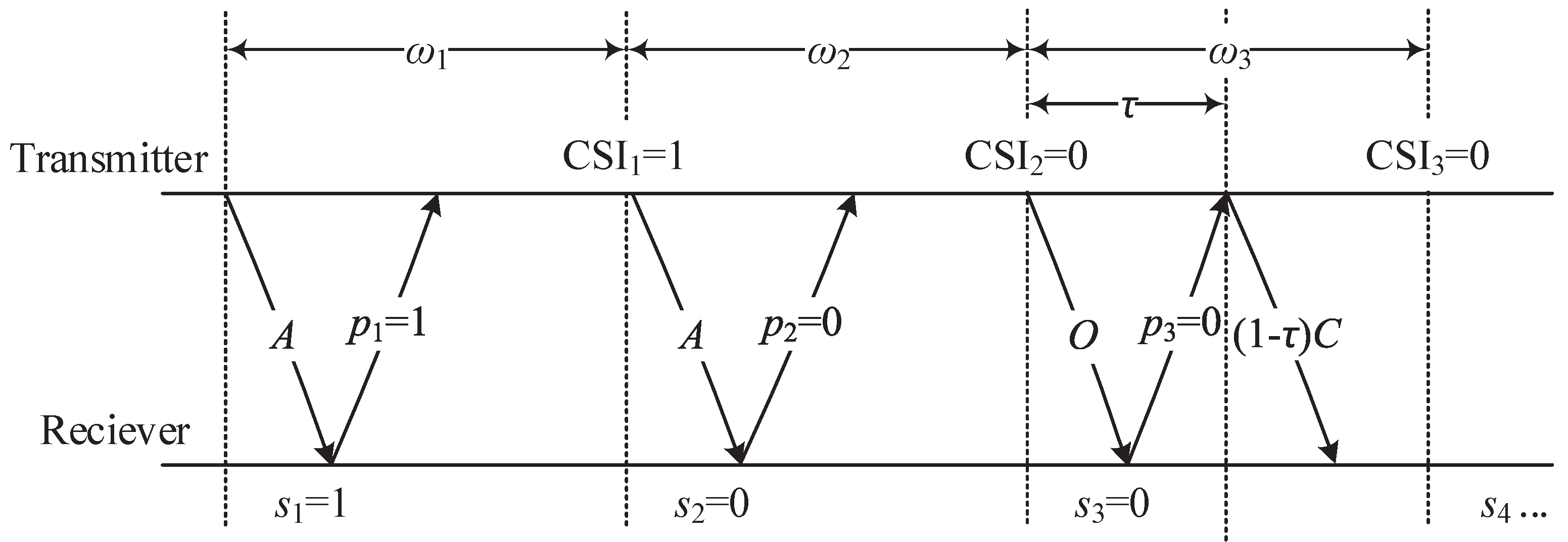
The transmission time slots can be expressed as $W=\{w_1,w_2,...,w_n\}$, the duration of a transmission time slot is a constant D, and and the corresponding states series of the GE channel can be expressed as $S=\{s_1,s_2,...,s_n\}$. The proposed POMDP-based transmission scheme with delayed CSI is shown in Figure 1.

The transmitter can thus obtain the delayed CSI through belief probability p, e.g., if the previous state is in the good state, then the receiver feedback of a single bit information is 1, otherwise 0. Therefore, there are three transmission actions for the transmitter that can be chosen at the beginning of each transmission time slot $w_i$, and each action is explained in detail as follows.

Betting aggressively (action A): When the transmitter believes that the channel has a high chance in a good state, the transmitter decides to “gamble” and transmits a high number $R_g$ of data bits.

Betting conservatively (action C): When the transmitter believes the channel is in a bad state, and decides to “play safe” and transmits a low number $R_b$ of data bits.

Betting opportunistically (action O): For this action, the transmitter adopts to sense the channel state at the beginning of the slot by sending a control/probing bit. The cost of sensing is a fraction $\tau$ of the slot, which is the time spent sensing the channel, defined as $\tau =d_{RTT}/D$, where $d_{RTT}$ is the round trip time, and D is the (constant) duration of a transmission time slot. Then the transmitter selects the appropriate transmission action (A or C) according to the sensing outcome, and $(1-\tau )R_g$ data bits will send if the channel was found to be in the good state or $(1-\tau )R_b$ data bits if otherwise.

Therefore, at the beginning of i-th transmission time slot $w_i$, the transmitter needs to decide an optimal action $a_i$ from the three actions above, i.e., $a_i\in \{A,C,O\}$ to maximize the expected throughput of our proposed POMDP-based transmission scheme. Because the transmitter only can have delayed feedback CSI or even no feedback, this is a POMDP problem.

Let $X_i$ denote the channel belief, which is the conditional probability that the channel is in the good state at the beginning of the i-th transmission time slot, from the past channel history of actions and accumulated delay CSI $H_{i+t}$, thus $X_{i+t}=Pr[s_{i+t}=1|H_{i+t}]$. Define a policy $\pi$ as a map from the belief at a particular time t to an action in the action space. Hence, by using this belief as the decision variable, let $V_{\beta }^{\pi }\left(p\right)$ denote the expected reward, with a discount factor $\beta$ ($0\le \beta <1$), the maximize expected throughput has the following expression:

$$V_{\beta }^{\pi }\left(p\right)=E[\sum _{t=0}^{\infty }{\beta }^{t}R(X_{i+t},a_{i+t})|X_i=p],$$

(2)

where $X_i=p$ is the initial value of the belief at the i-th transmission time slot, and we formulate the optimization problem with $t=0$ in the next section.

3. Optimal Transmission Policy Based on POMDP

In this section, we derive the optimal policy for the transmitter that knows the CSI feedback at the end of each slot as shown in Figure 1. The necessary conditions that tell if the action of betting opportunistically should be used under certain SIN communication scenarios was derived, and then the key thresholds for selecting the optimal transmission actions for the SIN communications are derived.

From the above discussion, we understand that an optimal policy exists for our POMDP problem as shown in Equation (2), and the expected reward is $R(X_i,a_i)$; if the aggressive action A is selected, since the probability of the channel in a good state at the next time is $X_i$, then the expected number of successfully transmitted data bits is $X_i{R}_g$; if the conservative action C is selected, $R_b$ data bits will be transmitted without error; at last, if opportunistically action O is selected, the expected transmitted data bits are $(1-\tau )[(1-X_i)R_b+X_i{R}_g]$. Then, we define the value function $V_{\beta }\left(p\right)$ as $V_{\beta }\left(p\right)=\underset{\pi }{max}{V}_{\beta }^{\pi }\left(p\right)$, for all $p\in [0,1]$, and $\pi$ denotes the map from the belief at a particular time to an action in the action space $\{A,C,O\}$. The value function $V_{\beta }\left(p\right)$ satisfies the Bellman equation

$$V_{\beta }\left(X_i\right)=\underset{a_i\in \{A,C,O\}}{max}\left\{V_{\beta ,a_i}\left(X_i\right)\right\},$$

(3)

where $V_{\beta ,a_i}\left(X_i\right)$ is the value acquired by taking action $a_i$ when the belief is $X_i$. By using the delayed feedback belief probability $X_i=p_i$, the transmitter selects the optimal transmission action $a_i\in \{A,C,O\}$ to maximize the throughput with the feedback belief $X_i=p_i$ being given by

$$V_{\beta ,a_i}\left(X_i\right)=R(p_i,a_i)+\beta E\left[V_{\beta }\left(X\right)\right|X_i=p_i,a_i=A],$$

(4)

where $X_i$ is the channel belief of the optimal action which selected at the beginning of the next time slot, and $X=T\left(p\right)={\lambda }_0(1-p)+{\lambda }_{1}p=\alpha p+{\lambda }_0$ in which $\alpha ={\lambda }_1-{\lambda }_0$. Then, $V_{\beta ,a_i}\left(p_i\right)$ can be explained for the three possible actions:

(1)

Betting aggressively: If aggressive action A is taken, then, the value function evolves as $V_{\beta ,A}(X_i=p_i)=p_i{R}_g+\beta V_{\beta }\left(T\left(p_i\right)\right)$;

(2)

Betting conservatively: If the conservative action C is selected, the value function evolves as $V_{\beta ,C}(X_i=p_i)=R_b+\beta V_{\beta }\left(T\left(p_i\right)\right)$;

(3)

Betting opportunistically: If opportunistic action O is selected, the value function evolves as $V_{\beta ,O}(X_i=p_i)=(1-\tau )[p_i{R}_g+(1-p_i)R_b]+\beta V_{\beta }\left(T\left(p_i\right)\right)$.

Hence, if the channel belief $X_i=p_i$ is probability of the slot $w_i$ in a good state, then the channel belief of next slot $w_{i+1}$ is ${\lambda }_1$. Similarly, if the CSI in a bad state is $(1-p_i)$ in $w_i$, then the channel belief of $w_{i+1}$ is ${\lambda }_0$, i.e., $V_{\beta }\left(T\left(p_i\right)\right)=(1-p_i)V_{\beta }\left({\lambda }_0\right)+p_i{V}_{\beta }\left({\lambda }_1\right)$, and then we can rewrite the above equations as follows

$$\left\{\begin{array}{c}{V}_{\beta ,A}(X_i=p_i)=p_i{R}_g+\beta (p_i{V}_{\beta }\left({\lambda }_1\right)+(1-p_i)V_{\beta }\left({\lambda }_0\right))\hfill \\ V_{\beta ,C}(X_i=p_i)=R_b+\beta (p_i{V}_{\beta }\left({\lambda }_1\right)+(1-p_i)V_{\beta }\left({\lambda }_0\right))\hfill \\ V_{\beta ,O}(X_i=p_i)=(1-\tau )[p_i{R}_g+(1-p_i)R_b]+\beta (p_i{V}_{\beta }\left({\lambda }_1\right)+(1-p_i)V_{\beta }\left({\lambda }_0\right))\hfill \end{array}\right..$$

(5)

Finally, the Bellman equation for our POMDP-based transmission policy over Ka-Band channels for SINs can be expressed as

$$V_{\beta }(X_i=p_i)=\underset{a_i\in \{A,C,O\}}{max}\{V_{\beta ,A}\left(p_i\right),V_{\beta ,C}\left(p_i\right),V_{\beta ,O}\left(p_i\right)\}.$$

(6)

Moreover, Smallwood et al. [27] proved that $V_{\beta }\left(X_i\right)$ is convex and nondecreasing, and there exist three thresholds $0\le {\rho }_1\le {\rho }_2\le {\rho }_3\le 1$. 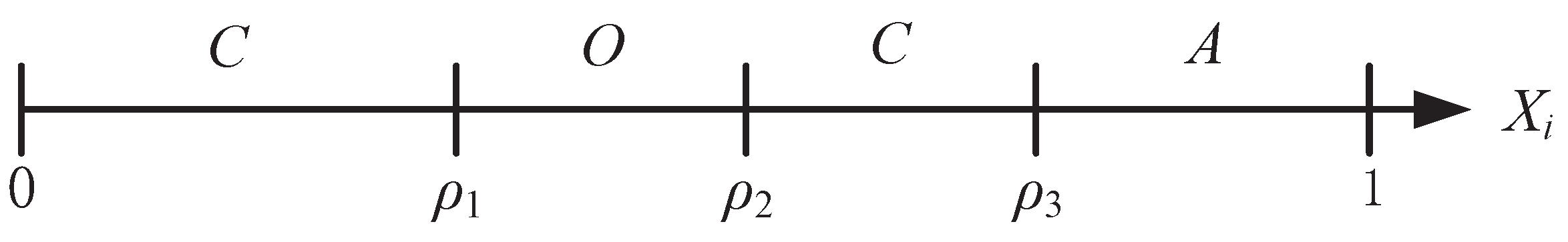Therefore, there are three types of threshold policies accordingly: (1) When ${\rho }_1={\rho }_2={\rho }_3$, the optimal policy is a one-threshold policy; (2) When ${\rho }_1<{\rho }_2={\rho }_3$, the optimal policy is a two-thresholds policy; (3) When ${\rho }_1<{\rho }_2<{\rho }_3$, the optimal policy is a three-thresholds policy. The optimal policy for the three-thresholds policy is illustrated in Figure 2, and the interval $[0,1]$ is separated in four regions by the thresholds ${\rho }_1$, ${\rho }_2$ and ${\rho }_3$.

Intuitively, one would think that there should exist only three regions, i.e., if $X_i$ is small, one should play safe; if $X_i$ is high, one should gamble, and, somewhere in between, sensing is optimal. However, if the transmitter can not obtain the feedback CSI, for some cases , a three-threshold policy is optimal and an example is shown in [28].

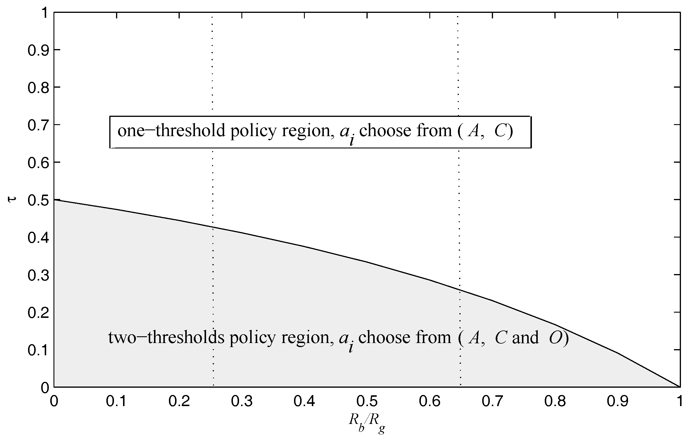
However, with the help of the delayed feedback CSI, our POMDP-based transmission policy has only three regions, i.e., (${\rho }_2,{\rho }_3$) = ∅. Therefore, the necessary conditions that tell if action O should be selected under a given SIN communication scenario, with data rate $R_g$ and $R_b$ in good and bad states, respectively, two thresholds $\{{\rho }_1,{\rho }_2\}$, and cost of action O is $\tau$, are given in the following theorem.

Theorem 1.

In terms of the POMDP-based optimal transmission scheme constructed by the Bellman function Equation (6), where $X_i{R}_g$ is the expected return when the risky action A is taken, $R_b$ bits are transmitted regardless of the channel conditions when action C is selected, and the expected return when the sensing action O is taken is $(1-\tau )[(1-X_i)R_b+X_i{R}_g]$, therefore:

If $R_b/R_g<(1-2\tau )/(1-\tau )$ then the optimal policy is a two-thresholds $\{{\rho }_1,{\rho }_2\}$ policy, and the optimal action $a_i$ can be selected from $\{A,C,O\}$;

Otherwise, if $R_b/R_g\ge (1-2\tau )/(1-\tau )$ then the optimal policy is a one-threshold ρ policy and the optimal action $a_i$ can be selected from $\{A,C\}$.

Proof of Theorem 1.

In our SIN POMDP-based transmission scheme, without loss of generality, assume that the optimal policy has two thresholds $0<{\rho }_1\le {\rho }_2<1$. Note that, since ${\rho }_1$ is the solution of $V_{\beta ,C}\left(X_i\right)=V_{\beta ,O}\left(X_i\right)$, and ${\rho }_2$ is the solution of $V_{\beta ,O}\left(X_i\right)=V_{\beta ,A}\left(X_i\right)$, it is easy to establish that

$$\left\{\begin{array}{c}{V}_{\beta ,C}\left({\rho }_1\right)=V_{\beta ,O}\left({\rho }_1\right)\hfill \\ V_{\beta ,A}\left({\rho }_2\right)=V_{\beta ,O}\left({\rho }_2\right)\hfill \end{array}\right..$$

(7)

From Equation (5), we have

$$\left\{\begin{array}{c}{\rho }_1=\frac{\tau R_b}{(1-\tau )(R_g-R_b)}\hfill \\ {\rho }_2=\frac{(1-\tau )R_b}{(1-\tau )R_b+\tau R_g}\hfill \end{array}\right..$$

(8)

If the optimal policy has two thresholds then ${\rho }_1<{\rho }_2$, and the communication parameters should satisfy

$$\frac{R_b}{R_g}<\frac{1-2\tau }{1-\tau }.$$

(9)

Otherwise, if the optimal policy has one threshold $\rho =({\rho }_1={\rho }_2)$, then the communication parameters turn to satisfy

$$\frac{R_b}{R_g}\ge \frac{1-2\tau }{1-\tau }.$$

(10)

☐

Note that Theorem 1 establishes the structure that tells if action O should be used, and two types of threshold policies exist depending on the system parameters–in particular, the cost of the sensing action $\tau$ versus the ratio of $R_b/R_g$, and the optimal policy space is partitioned into two regions, which is illustrated in Figure 3.

Figure 3 illustrated that the established two optimal policies regions can be further partitioned into three regions at most. As one should expect, the optimal transmission scheme here is a myopic policy that maximizes the immediate reward. Next, we detailed the optimal transmission action in the one-threshold policy region and the two-thresholds policy region in Figure 3, and gave a complete characterization of the thresholds for each policy in the following, respectively.

Assume that the one-threshold policy has one threshold $0<\rho <1$, and the transition probability matrix $\mathbf{G}$ of the two-state GE channel is $\mathbf{G}=\left[\begin{array}{cc}{\lambda }_1& 1-{\lambda }_1\\ {\lambda }_0& 1-{\lambda }_0\end{array}\right]$. Then, the optimal transmission action $a_i$ is introduced in the following Theorem 2.

Theorem 2.

Let $a_i=\{A,C\}$ denote the action space in the one-threshold policy region, $R_g$ and $R_b$ denote the transmitted numbers of data bits that corresponding to the action A and C, respectively, then $a_i$ is determined as follows:

(1)

If $R_b/R_g<{\lambda }_0$, then the optimal transmission action is $a_i=A$ regardless of the delayed feedback CSI is $s_{i-1}=1$ or $s_{i-1}=0$;

(2)

If $R_b/R_g>{\lambda }_1$, then the optimal transmission action is $a_i=C$ regardless of the delayed feedback CSI is $s_{i-1}=1$ or $s_{i-1}=0$;

(3)

Finally if ${\lambda }_0\le R_b/R_g\le {\lambda }_1$, then the optimal transmission action $a_i=A$ when the delayed feedback CSI is $s_{i-1}=1$, and the optimal transmission action is $a_i=C$ when the delayed feedback CSI is $s_{i-1}=0$.

Proof of Theorem 2.

Recall in our POMDP model that any general value function $V_{\beta }(·)$ is convex.

Hence, (1) if $R_b/R_g<{\lambda }_0$, when the delayed feedback CSI is $s_{i-1}=1$, and the channel belief is $X_i={\lambda }_1$, then we have $V_{\beta ,A}(X_i={\lambda }_1)>V_{\beta ,C}(X_i={\lambda }_1)$ since

$$\left\{\begin{array}{c}{V}_{\beta ,A}(X_i={\lambda }_1)={\lambda }_1{R}_g+\beta ({\lambda }_1{V}_{\beta }\left({\lambda }_1\right)+(1-{\lambda }_1)V_{\beta }\left({\lambda }_0\right)),\hfill \\ V_{\beta ,C}(X_i={\lambda }_1)=R_b+\beta ({\lambda }_1{V}_{\beta }\left({\lambda }_1\right)+(1-{\lambda }_1)V_{\beta }\left({\lambda }_0\right)),\hfill \end{array}\right.$$

(11)

and ${\lambda }_1>{\lambda }_0>R_b/R_g$. Similarly, when the delayed feedback CSI is $s_{i-1}=0$, we still have $V_{\beta ,A}(X_i={\lambda }_0)>V_{\beta ,C}(X_i={\lambda }_0)$ since

$$\left\{\begin{array}{c}{V}_{\beta ,A}(X_i={\lambda }_0)={\lambda }_0{R}_g+\beta ({\lambda }_0{V}_{\beta }\left({\lambda }_0\right)+(1-{\lambda }_0)V_{\beta }\left({\lambda }_0\right))\hfill \\ V_{\beta ,C}(X_i={\lambda }_0)=R_b+\beta ({\lambda }_0{V}_{\beta }\left({\lambda }_0\right)+(1-{\lambda }_0)V_{\beta }\left({\lambda }_0\right))\hfill \end{array}\right..$$

(12)

Hence, the optimal transmission action in this case is $a_i=A$.

(2) If $R_b/R_g>{\lambda }_1$, similar to the previous case, regardless of the delayed feedback CSI is $s_{i-1}=1$ or $s_{i-1}=0$ (i.e., the channel belief is $X_i={\lambda }_1$ or $X_i={\lambda }_0$, respectively), we have $V_{\beta ,A}\left(p_i\right)<V_{\beta ,C}\left(p_i\right)$, therefore, by substituting $p_i$ into Equations (11) and (12) directly. Therefore, the action $a_i=C$ is optimal in this case.

(3) If ${\lambda }_0\le R_b/R_g\le {\lambda }_1$, the approach here is similar to the previous cases, i.e., when the delayed feedback CSI is $s_{i-1}=1$ and $p_i={\lambda }_1$, we will have $V_{\beta ,A}(X_i={\lambda }_1)>V_{\beta ,C}(X_i={\lambda }_1)$, therefore by substituting $p_i={\lambda }_1$ into Equation (11), and the action $a_i=A$ is the optimal strategy here; otherwise, when the delayed feedback CSI is $s_{i-1}=0$ and $p_i={\lambda }_0$, we consequently obtain $V_{\beta ,A}(X_i={\lambda }_0)<V_{\beta ,C}(X_i={\lambda }_0)$ by substituting $p_i={\lambda }_0$ into Equation (12) and the optimal transmission action in this case is $a_i=C$. ☐

The complete characterization of the optimal transmission action of the one-threshold policy is given in

Table 1. Optimal transmission action in the one-threshold policy region.

Parameters	Delayed Feedback CSI ${\mathit{s}}_{\mathit{i}-1}$	Optimal Transmission Action ${\mathit{a}}_{\mathit{i}}$
$R_b/R_g<{\lambda }_0$	$s_{i-1}=1/0$	$a_i=A$
${\lambda }_0\le R_b/R_g\le {\lambda }_1$	$s_{i-1}=1$	$a_i=A$
	$s_{i-1}=0$	$a_i=C$
$R_b/R_g>{\lambda }_1$	$s_{i-1}=1/0$	$a_i=C$

.

Furthermore, it is worth noting that Theorem 2 proves that the value function is totally determined by finding $V_{\beta }\left({\lambda }_1\right)$ and $V_{\beta }\left({\lambda }_0\right)$. In order to calculate the expected reward of the optimal action when the belief is ${\lambda }_1$ or ${\lambda }_0$, we start by comparing these value functions established in Theorem 2 to the threshold $\rho$ in Theorem 1. Then, all that remains is solving a system of two linear equations with two unknowns, i.e., $V_{\beta }\left({\lambda }_1\right)$ and $V_{\beta }\left({\lambda }_0\right)$, in three cases: $\rho <{\lambda }_0$, ${\lambda }_0\le \rho \le {\lambda }_1$ and ${\lambda }_1<\rho$.

To illustrate the procedure of determining $V_{\beta }\left({\lambda }_1\right)$ and $V_{\beta }\left({\lambda }_0\right)$, we consider the example where $\rho <{\lambda }_0$, and the optimal transmission action is $a_i=A$ regardless of the delayed feedback CSI in this case, as we have proved in Theorem 2; we have then

$$V_{\beta }\left({\lambda }_0\right)=V_{\beta ,A}(X_i={\lambda }_0)={\lambda }_0{R}_g+\beta ({\lambda }_0{V}_{\beta }\left({\lambda }_1\right)+(1-{\lambda }_0)V_{\beta }\left({\lambda }_0\right)),$$

(13)

$$V_{\beta }\left({\lambda }_1\right)=V_{\beta ,A}(X_i={\lambda }_1)={\lambda }_1{R}_g+\beta ({\lambda }_1{V}_{\beta }\left({\lambda }_1\right)+(1-{\lambda }_1)V_{\beta }\left({\lambda }_0\right)).$$

(14)

Recall that we have $\alpha ={\lambda }_1-{\lambda }_0$, and solving for $V_{\beta }\left({\lambda }_1\right)$ and $V_{\beta }\left({\lambda }_0\right)$ leads to

$$V_{\beta }\left({\lambda }_0\right)={\lambda }_0{R}_g/\left(\right(1-\beta \left)\right(1-\alpha \beta \left)\right),$$

(15)

$$V_{\beta }\left({\lambda }_1\right)=({\lambda }_1-\alpha \beta )R_g/\left(\right(1-\beta \left)\right(1-\alpha \beta \left)\right).$$

(16)

All other cases can be solved similarly, and the closed form computation expressions of the one-threshold policy are given in

Table 2. Closed form computation expressions of the one-threshold policy.

Conditions	Corresponding Value Functions	Closed Form Computation Expressions
$\rho <{\lambda }_0$	$V_{\beta }\left({\lambda }_0\right)=V_{\beta ,A}(X_i={\lambda }_0)$ $V_{\beta }\left({\lambda }_1\right)=V_{\beta ,A}(X_i={\lambda }_1)$	$V_{\beta }\left({\lambda }_0\right)=\frac{{\lambda }_0{R}_g}{(1-\beta )(1-\alpha \beta )}$ $V_{\beta }\left({\lambda }_1\right)=\frac{({\lambda }_1-\alpha \beta )R_g}{(1-\beta )(1-\alpha \beta )}$
${\lambda }_0\le \rho \le {\lambda }_1$	$V_{\beta }\left({\lambda }_0\right)=V_{\beta ,C}(X_i={\lambda }_0)$ $V_{\beta }\left({\lambda }_1\right)=V_{\beta ,A}(X_i={\lambda }_1)$	$V_{\beta }\left({\lambda }_0\right)=\frac{(1-\beta {\lambda }_1)R_b+\beta {\lambda }_0{\lambda }_1{R}_g}{(1-\beta )(1-\alpha \beta )}$ $V_{\beta }\left({\lambda }_1\right)=\frac{\beta (1-{\lambda }_1)R_b+(1-\beta +\beta {\lambda }_0)R_g}{(1-\beta )(1-\alpha \beta )}$
${\lambda }_1<\rho$	$V_{\beta }\left({\lambda }_0\right)=V_{\beta ,C}(X_i={\lambda }_0)$ $V_{\beta }\left({\lambda }_1\right)=V_{\beta ,C}(X_i={\lambda }_1)$	$V_{\beta }\left({\lambda }_0\right)=\frac{R_b}{(1-\beta )}$ $V_{\beta }\left({\lambda }_1\right)=\frac{R_b}{(1-\beta )}$

.

Next, assume that in the two-thresholds policy region, the optimal policy has two thresholds $0<{\rho }_1<{\rho }_2<1$, and the transition probability matrix is $\mathbf{G}=\left[\begin{array}{cc}{\lambda }_1& 1-{\lambda }_1\\ {\lambda }_0& 1-{\lambda }_0\end{array}\right]$. Then, the optimal transmission action $a_i$ is given in the following Theorem 3.

Theorem 3.

Let $a_i=\{A,C,O\}$ denote the action space in the two-thresholds policy region, and $R_g$ and $R_b$ denote the transmitted numbers of data bits that correspond to the actions A and C, respectively. Recall that τ is the sensing cost that is the ratio of the round trip time $d_{RTT}$ to the time slot duration D and satisfies $\tau <(1-R_b/R_g)/(2-R_b/R_g)$ as in Theorem 1, and $X_i$ is the channel belief, then $a_i$ is determined as follows:

(1)

If $R_b/R_g<{\lambda }_0$, then two cases can be distinguished: if $R_b/R_g<\tau X_i/\left((1-\tau )(1-X_i)\right)$, the optimal transmission action is $a_i=A$, regardless of the delayed feedback CSI being $s_{i-1}=1$ or $s_{i-1}=0$; else, if $R_b/R_g\ge \tau X_i/\left((1-\tau )(1-X_i)\right)$, the optimal transmission action is $a_i=O$, regardless of the delayed feedback CSI being $s_{i-1}=1$ or $s_{i-1}=0$.

(2)

If $R_b/R_g>{\lambda }_1$, then two cases can be distinguished: if $R_b/R_g<(1-\tau )X_i/(\tau +X_i-\tau X_i)$, the optimal transmission action is $a_i=O$, regardless of the delayed feedback CSI being $s_{i-1}=1$ or $s_{i-1}=0$; else, if $R_b/R_g\ge (1-\tau )X_i/(\tau +X_i-\tau X_i)$, the optimal transmission action is $a_i=C$ regardless of the delayed feedback CSI being $s_{i-1}=1$ or $s_{i-1}=0$.

(3)

Finally if ${\lambda }_0\le R_b/R_g\le {\lambda }_1$, when the delayed feedback CSI is $s_{i-1}=1$ and $X_i={\lambda }_1$, then the optimal transmission action is $a_i=A$; when the delayed feedback CSI is $s_{i-1}=0$ and $X_i={\lambda }_0$, then the optimal transmission action is $a_i=C$.

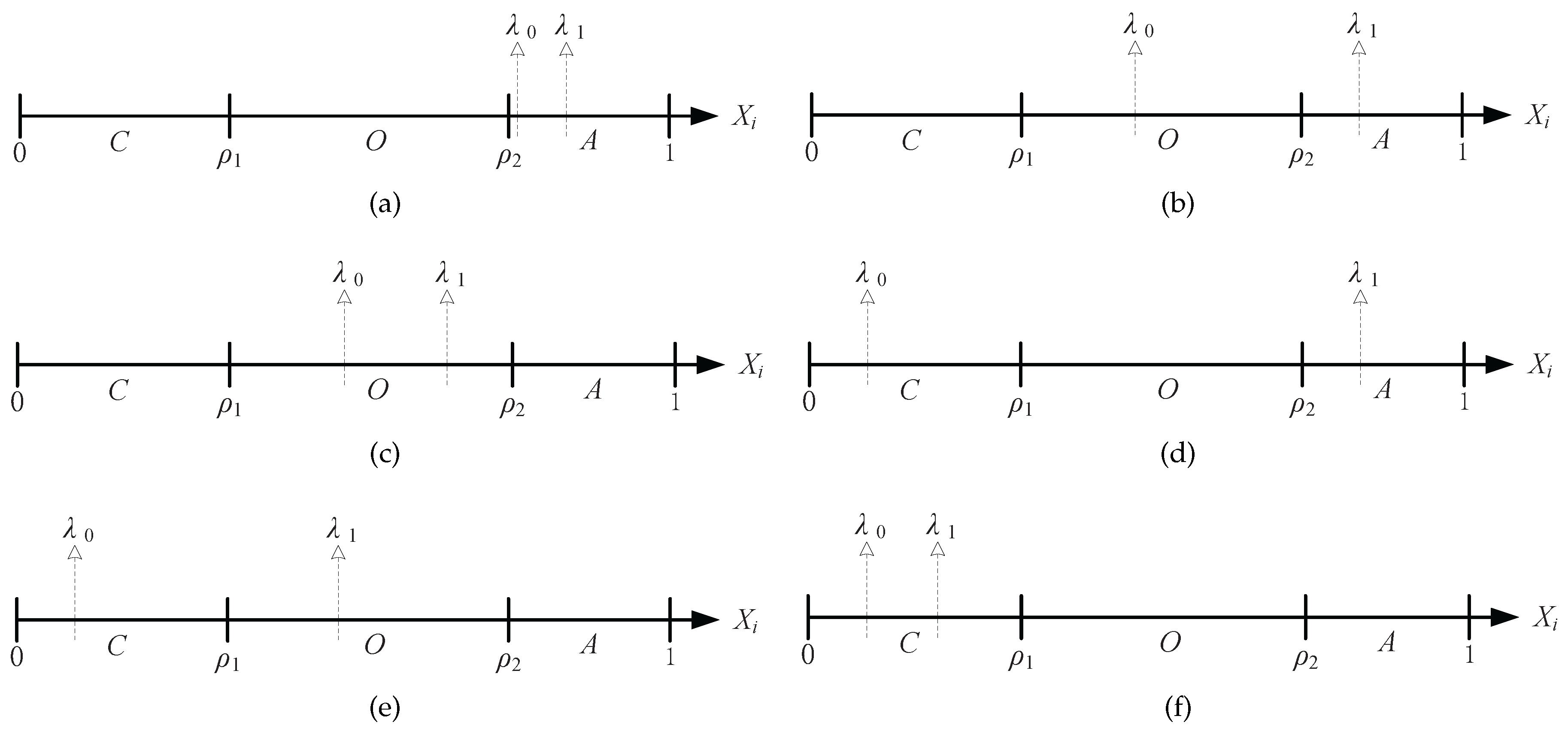
Proof of Theorem 3.

The proof here needs to utilize the previous case in Theorem 1; recall in our POMDP model that any general value function $V_{\beta }(·)$ is convex, the interval [0, 1] of $R_b/R_g$ is separate in three regions by the thresholds ${\rho }_1$ and ${\rho }_2$, all the six possible optimal policy structures of the two-thresholds policy are illustrated in Figure 4, and, then, we can distinguish them into three possible scenarios.

(1) If $R_b/R_g<{\lambda }_0$, we can distinguish three subcases:

If ${\rho }_2<{\lambda }_0$ as shown in Figure 4a, then we have that the optimal action is $a_i=A$ for $s_i=0/1$ where $V_{\beta ,A}(X_i={\lambda }_0)>V_{\beta ,O}(X_i={\lambda }_0)$ and $V_{\beta ,A}(X_i={\lambda }_1)>V_{\beta ,O}(X_i={\lambda }_1)$, and since

$$\left\{\begin{array}{c}{V}_{\beta ,A}(X_i=p_i)=p_i{R}_g+\beta (p_i{V}_{\beta }\left({\lambda }_1\right)+(1-p_i)V_{\beta }\left({\lambda }_0\right))\hfill \\ V_{\beta ,O}(X_i=p_i)=(1-\tau )[p_i{R}_g+(1-p_i)R_b]+\beta (p_i{V}_{\beta }\left({\lambda }_1\right)+(1-p_i)V_{\beta }\left({\lambda }_0\right))\hfill \end{array}\right..$$

(17)

Hence, the optimal transmission action in this case is $a_i=A$ for $R_b/R_g<\tau {\lambda }_0/\left((1-\tau )(1-{\lambda }_0)\right)$ and $R_b/R_g<\tau {\lambda }_1/\left((1-\tau )(1-{\lambda }_1)\right)$.

Else, if ${\rho }_1<{\lambda }_0<{\rho }_2<{\lambda }_1$, as is illustrated in Figure 4b, then we have $a_i=A$ for $s_{i-1}=1$ where $V_{\beta ,A}(X_i={\lambda }_1)>V_{\beta ,O}(X_i={\lambda }_1)$ as the above subcase obtained, and $a_i=O$ is the optimal action for $s_{i-1}=0$ where $V_{\beta ,O}(X_i={\lambda }_0)>V_{\beta ,A}(X_i={\lambda }_0)$ in Figure 4b, and $R_b/R_g\ge \tau {\lambda }_0/\left((1-\tau )(1-{\lambda }_0)\right)$ by substituting $X_i={\lambda }_0$ into Equation (17) with ${\rho }_1<{\lambda }_0<{\rho }_2<{\lambda }_1$.

Lastly, if ${\rho }_1<{\lambda }_0<{\lambda }_1<{\rho }_2$, as is shown in Figure 4c, we have $a_i=O$ for $s_i=0/1$ being the optimal action due to the solution of $V_{\beta ,C}(X_i={\lambda }_0)<V_{\beta ,O}(X_i={\lambda }_0)$ and $V_{\beta ,C}(X_i={\lambda }_1)<V_{\beta ,O}(X_i={\lambda }_1)$ by substituting $X_i={\lambda }_0$ and $X_i={\lambda }_1$ into Equation (17), and we obtain $R_b/R_g\ge \tau {\lambda }_0/\left((1-\tau )(1-{\lambda }_0)\right)$.

(2) If $R_b/R_g>{\lambda }_1$, similarly, three subcases can be distinguished:

If ${\rho }_1<{\lambda }_0<{\lambda }_1<{\rho }_2$, as is shown in Figure 4c, then we have $V_{\beta ,C}(X_i={\lambda }_0)<V_{\beta ,O}(X_i={\lambda }_0)$ and $V_{\beta ,C}(X_i={\lambda }_1)<V_{\beta ,O}(X_i={\lambda }_1)$; thus, we have

$$\left\{\begin{array}{c}{V}_{\beta ,O}(X_i=p_i)=(1-\tau )[p_i{R}_g+(1-p_i)R_b]+\beta (p_i{V}_{\beta }\left({\lambda }_1\right)+(1-p_i)V_{\beta }\left({\lambda }_0\right))\hfill \\ V_{\beta ,C}(X_i=p_i)=R_b+\beta (p_i{V}_{\beta }\left({\lambda }_1\right)+(1-p_i)V_{\beta }\left({\lambda }_0\right))\hfill \end{array}\right.,$$

(18)

where $a_i=O$ is the optimal action since $R_b/R_g<(1-\tau ){\lambda }_1/(\tau +{\lambda }_1-\tau {\lambda }_1)$ and $R_b/R_g<(1-\tau ){\lambda }_0/(\tau +{\lambda }_0-\tau {\lambda }_0)$ by solving the value function Equation (18).

Else, if ${\lambda }_0<{\rho }_1<{\lambda }_1<{\rho }_2$, as is shown in Figure 4e, then we have $a_i=C$ for $s_{i-1}=0$ where $V_{\beta ,O}(X_i={\lambda }_0)<V_{\beta ,C}(X_i={\lambda }_0)$ for $R_b/R_g\ge (1-\tau ){\lambda }_0/(\tau +{\lambda }_0-\tau {\lambda }_0)$ by substituting $X_i={\lambda }_0$ into Equation (18), and $a_i=O$ is the optimal action for $s_{i-1}=1$ where $V_{\beta ,O}(X_i={\lambda }_1)>V_{\beta ,A}(X_i={\lambda }_1)$ for $R_b/R_g<(1-\tau ){\lambda }_1/(\tau +{\lambda }_1-\tau {\lambda }_1)$ by substituting $X_i={\lambda }_1$ into Equation (18).

Lastly, if ${\lambda }_1<{\rho }_1$, as is shown in Figure 4f, we have $a_i=C$ being the optimal action regardless if the delayed feedback CSI is $s_{i-1}=0$ or $s_{i-1}=1$, where $V_{\beta ,C}(X_i={\lambda }_0)>V_{\beta ,O}(X_i={\lambda }_0)$ and $V_{\beta ,C}(X_i={\lambda }_1)>V_{\beta ,O}(X_i={\lambda }_1)$. Then $R_b/R_g\ge (1-\tau ){\lambda }_0/(\tau +{\lambda }_0-\tau {\lambda }_0)$ and $R_b/R_g\ge (1-\tau ){\lambda }_1/(\tau +{\lambda }_1-\tau {\lambda }_1)$ by substituting $X_i={\lambda }_0$ and $X_i={\lambda }_1$ into Equation (18), respectively.

(3) Finally, if ${\lambda }_0\le R_b/R_g\le {\lambda }_1$, the computation is similar to the previous cases. For ${\lambda }_0<{\rho }_1<{\rho }_2<{\lambda }_1$, as is shown in Figure 4d, where the optimal action is $a_i=A$ for $s_{i-1}=1$, by using (17) to solve $V_{\beta ,A}(X_i={\lambda }_1)>V_{\beta ,O}(X_i={\lambda }_1)$ with $X_i={\lambda }_1$, then $R_b/R_g<\tau {\lambda }_1/\left((1-\tau )(1-{\lambda }_1)\right)$. In addition, if $s_{i-1}=0$, then $a_i=O$ is the optimal action, by solving Equation (18) with $X_i={\lambda }_0$ for $V_{\beta ,C}(X_i={\lambda }_0)>V_{\beta ,O}(X_i={\lambda }_0)$, and then we have $R_b/R_g\ge (1-\tau ){\lambda }_0/(\tau +{\lambda }_0-\tau {\lambda }_0)$.

☐

Let $\mathcal{A}\left(X_i\right)=\tau X_i/\left((1-\tau )(1-X_i)\right)$ and $\mathcal{C}\left(X_i\right)=(1-\tau )X_i/(\tau +X_i-\tau X_i)$, and

Table 3. Optimal transmitting action in the two-thresholds policy region.

Parameters	Conditions	Delayed Feedback CSI ${\mathit{s}}_{\mathit{i}-1}$	Optimal Action ${\mathit{a}}_{\mathit{i}}$
$\frac{R_b}{R_g}<{\lambda }_0$	Figure 4a: $R_b/R_g<\mathcal{A}\left({\lambda }_1\right)$	$s_{i-1}=1$	$a_i=A$
	Figure 4a: $R_b/R_g<\mathcal{A}\left({\lambda }_0\right)$	$s_{i-1}=0$
	Figure 4b: $R_b/R_g<\mathcal{A}\left({\lambda }_1\right)$	$s_{i-1}=1$
	Figure 4b: $R_b/R_g\ge \mathcal{A}\left({\lambda }_0\right)$	$s_{i-1}=0$	$a_i=O$
	Figure 4c: $R_b/R_g\ge \mathcal{A}\left({\lambda }_1\right)$	$s_{i-1}=1$
$\frac{R_b}{R_g}>{\lambda }_1$	Figure 4c: $R_b/R_g\ge \mathcal{C}\left({\lambda }_0\right)$	$s_{i-1}=0$
	Figure 4e: $R_b/R_g\ge \mathcal{C}\left({\lambda }_1\right)$	$s_{i-1}=1$
	Figure 4e: $R_b/R_g<\mathcal{C}\left({\lambda }_0\right)$	$s_{i-1}=0$	$a_i=C$
	Figure 4f: $R_b/R_g<\mathcal{C}\left({\lambda }_1\right)$	$s_{i-1}=1$
	Figure 4f: $R_b/R_g<\mathcal{C}\left({\lambda }_0\right)$	$s_{i-1}=0$
${\lambda }_1\le \frac{R_b}{R_g}\le {\lambda }_1$	Figure 4d: $R_b/R_g<\mathcal{A}\left({\lambda }_1\right)$	$s_{i-1}=1$	$a_i=A$
	Figure 4d: $R_b/R_g\ge \mathcal{C}\left({\lambda }_0\right)$	$s_{i-1}=0$	$a_i=C$

shows the complete characterization of the optimal transmission action in the two-thresholds policy region.

Similar to the previous case, we illustrate mathematical expressions for the $V_{\beta }\left({\lambda }_1\right)$ and $V_{\beta }\left({\lambda }_0\right)$ of Theorem 3 in

Table 4. Closed form computation expressions of the two-thresholds policy.

Conditions	Corresponding Functions	Closed Form Computation Expressions
${\rho }_2\le {\lambda }_0$	$V_{\beta }\left({\lambda }_0\right)=V_{\beta ,A}(X_i={\lambda }_0)$ $V_{\beta }\left({\lambda }_1\right)=V_{\beta ,A}(X_i={\lambda }_1)$	$V_{\beta }\left({\lambda }_0\right)=\frac{{\lambda }_0{R}_g}{(1-\beta )(1-\alpha \beta )}$ $V_{\beta }\left({\lambda }_1\right)=\frac{({\lambda }_1-\alpha \beta )R_g}{(1-\beta )(1-\alpha \beta )}$
${\rho }_1<{\lambda }_0<{\rho }_2\le {\lambda }_1$	$V_{\beta }\left({\lambda }_0\right)=V_{\beta ,O}(X_i={\lambda }_0)$ $V_{\beta }\left({\lambda }_1\right)=V_{\beta ,A}(X_i={\lambda }_1)$	$V_{\beta }\left({\lambda }_0\right)=\frac{(1-\tau )(1-\beta {\lambda }_1+\beta {\lambda }_0{\lambda }_1)R_b+(1-\tau ){\lambda }_0(R_g-R_b)+\tau \beta {\lambda }_0{\lambda }_1{R}_g}{(1-\beta )(1-\alpha \beta )}$ $V_{\beta }\left({\lambda }_1\right)=\frac{(1-\tau )\beta (1-{\lambda }_0)(1-{\lambda }_1)R_b+({\lambda }_1-\alpha \beta -\tau \beta {\lambda }_0+\tau \beta {\lambda }_0{\lambda }_1)R_g}{(1-\beta )(1-\alpha \beta )}$
${\rho }_1<{\lambda }_0<{\lambda }_1\le {\rho }_2$	$V_{\beta }\left({\lambda }_0\right)=V_{\beta ,O}(X_i={\lambda }_0)$ $V_{\beta }\left({\lambda }_1\right)=V_{\beta ,O}(X_i={\lambda }_1)$	$V_{\beta }\left({\lambda }_0\right)=\frac{(1-\beta {\lambda }_1)R_b+\beta {\lambda }_0{\lambda }_1{R}_g}{(1-\beta )(1-\alpha \beta )}$ $V_{\beta }\left({\lambda }_1\right)=\frac{\beta (1-{\lambda }_1)R_b+(1-\beta +\beta {\lambda }_0){\lambda }_1{R}_g}{(1-\beta )(1-\alpha \beta )}$
${\lambda }_0<{\rho }_1<{\rho }_2\le {\lambda }_1$	$V_{\beta }\left({\lambda }_0\right)=V_{\beta ,C}(X_i={\lambda }_0)$ $V_{\beta }\left({\lambda }_1\right)=V_{\beta ,A}(X_i={\lambda }_1)$	$V_{\beta }\left({\lambda }_0\right)=\frac{(1-\tau )((1-\alpha \beta )R_b+{\lambda }_0(R_g-R_b))}{(1-\beta )(1-\alpha \beta )}$ $V_{\beta }\left({\lambda }_1\right)=\frac{(1-\tau )((1-{\lambda }_1)R_b+({\lambda }_1-\alpha \beta )R_g)}{(1-\beta )(1-\alpha \beta )}$
${\lambda }_0<{\rho }_1<{\lambda }_1\le {\rho }_2$	$V_{\beta }\left({\lambda }_0\right)=V_{\beta ,C}(X_i={\lambda }_0)$ $V_{\beta }\left({\lambda }_1\right)=V_{\beta ,O}(X_i={\lambda }_1)$	$V_{\beta }\left({\lambda }_0\right)=\frac{(1-\beta +\beta {\lambda }_0)R_b+(1-\tau )\beta {\lambda }_0{\lambda }_1(R_g-R_b)}{(1-\beta )(1-\alpha \beta )}$ $V_{\beta }\left({\lambda }_1\right)=\frac{\beta (1-\tau )R_b+(1-\tau )(1-\beta +\beta {\lambda }_0)((1-{\lambda }_1)R_b+{\lambda }_1{R}_g)}{(1-\beta )(1-\alpha \beta )}$
${\lambda }_1\le {\rho }_1$	$V_{\beta }\left({\lambda }_0\right)=V_{\beta ,C}(X_i={\lambda }_0)$ $V_{\beta }\left({\lambda }_1\right)=V_{\beta ,C}(X_i={\lambda }_1)$	$V_{\beta }\left({\lambda }_0\right)=\frac{R_b}{(1-\beta )}$ $V_{\beta }\left({\lambda }_1\right)=\frac{R_b}{(1-\beta )}$

, in order to calculate the expected reward of the value function of the corresponding optimal action that is given in Theorem 3. Again, once $V_{\beta }\left({\lambda }_1\right)$ and $V_{\beta }\left({\lambda }_0\right)$ have been computed for the six possible optimal policy structures of the two-thresholds policy region in Theorem 3, we retain the scenario that gives the maximal values.

The procedure to calculate $V_{\beta }\left({\lambda }_1\right)$ and $V_{\beta }\left({\lambda }_0\right)$ starts by comparing these value functions established in Theorem 3 to the thresholds ${\rho }_1$ and ${\rho }_2$ established in Figure 4, and all the cases can be solved similarly to the previous example, and the closed form computation expressions of the two-thresholds policy are given in Table 4.

4. Simulation and Results

To evaluation our proposed POMDP-based optimal transmission policy, we start by comparing the transmission actions with different setups, each leading to a different optimal policy. We choose the parameters below in order to illustrate that, in theory, the optimal policy is determined by the communication scenario parameters, such as data rate $R_b$, $R_g$ and $\tau$ which is affected by the round trip time and the duration of the transmission time slot as in Theorem 1.

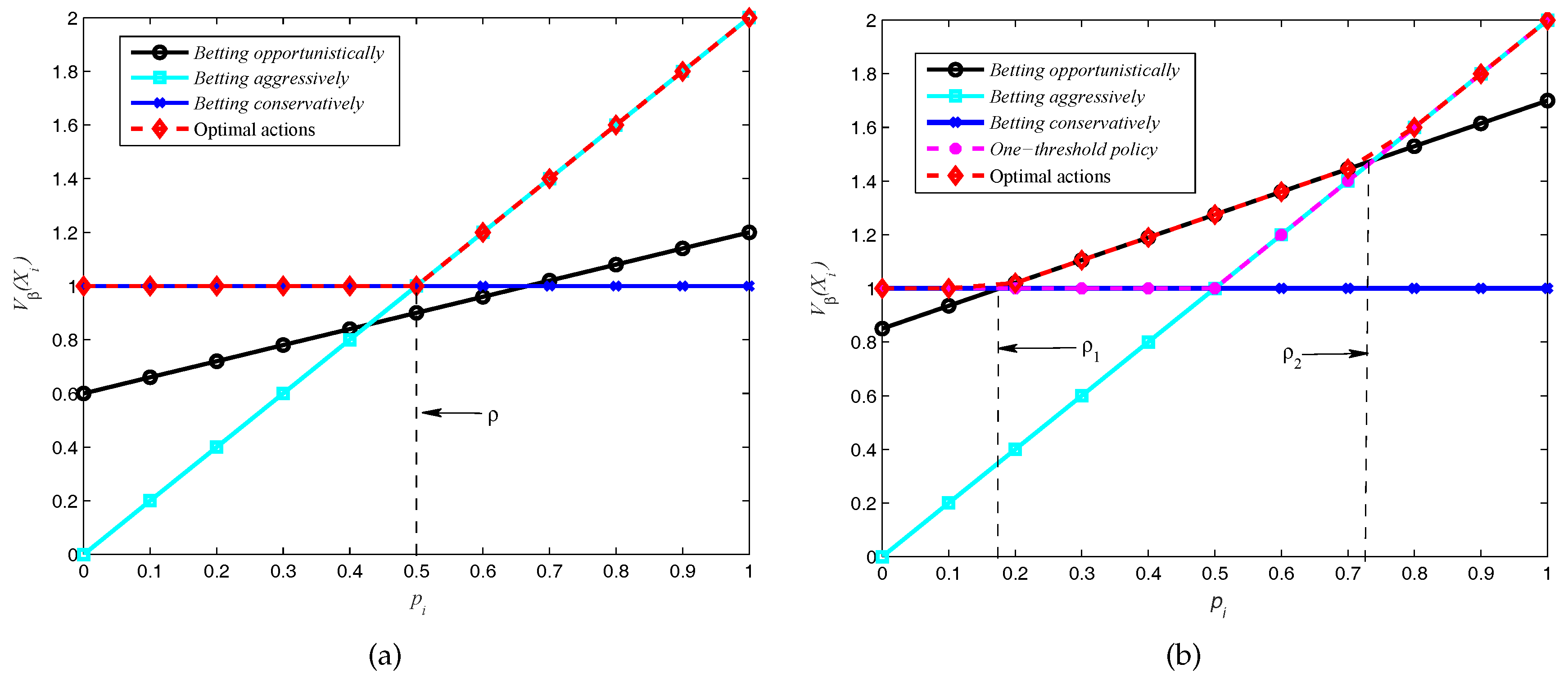
The first set of parameters considered is $\tau =0.4$, $R_g=2$, $R_b=1$, ${\lambda }_1=0.9$, ${\lambda }_0=0.2$, and $\beta =0.5$. Note that from Theorem 1, $\tau =0.4>1/3$ represents the action of betting opportunistically, which could not be used under this scenario, thus the one-threshold policy is optimal as the numerical result shows in Figure 5a. Furthermore, from Theorem 2, the threshold in Figure 5a is $\rho =0.5$. Therefore, if $p_i<\rho$, the optimal action is $a_i=C$, else if $p_i\ge \rho$, the optimal action is $a_i=A$, and betting opportunistically is unfeasible in this scenario.

If we keep all the parameter values fixed and diminish the cost of sensing to $\tau =0.15$, then from Theorem 1 we can compute that the optimal policy is the two-thresholds policy, shown in Figure 5b. From Figure 5b we can see that the one-threshold policy gives suboptimal values, and the two thresholds in this scenario are ${\rho }_1=0.176$ and ${\rho }_2=0.739$ by using Theorem 3. If $p_i<0.176$, the optimal transmission action is betting conservatively ($a_i=C$); else if $0.176\le p_i\le 0.739$, the optimal transmission action is betting opportunistically ($a_i=O$), which can achieve a better reward than $a_i=C$ or $a_i=A$ unless $p_i>0.739$, the optimal action is betting aggressively ($a_i=A$).

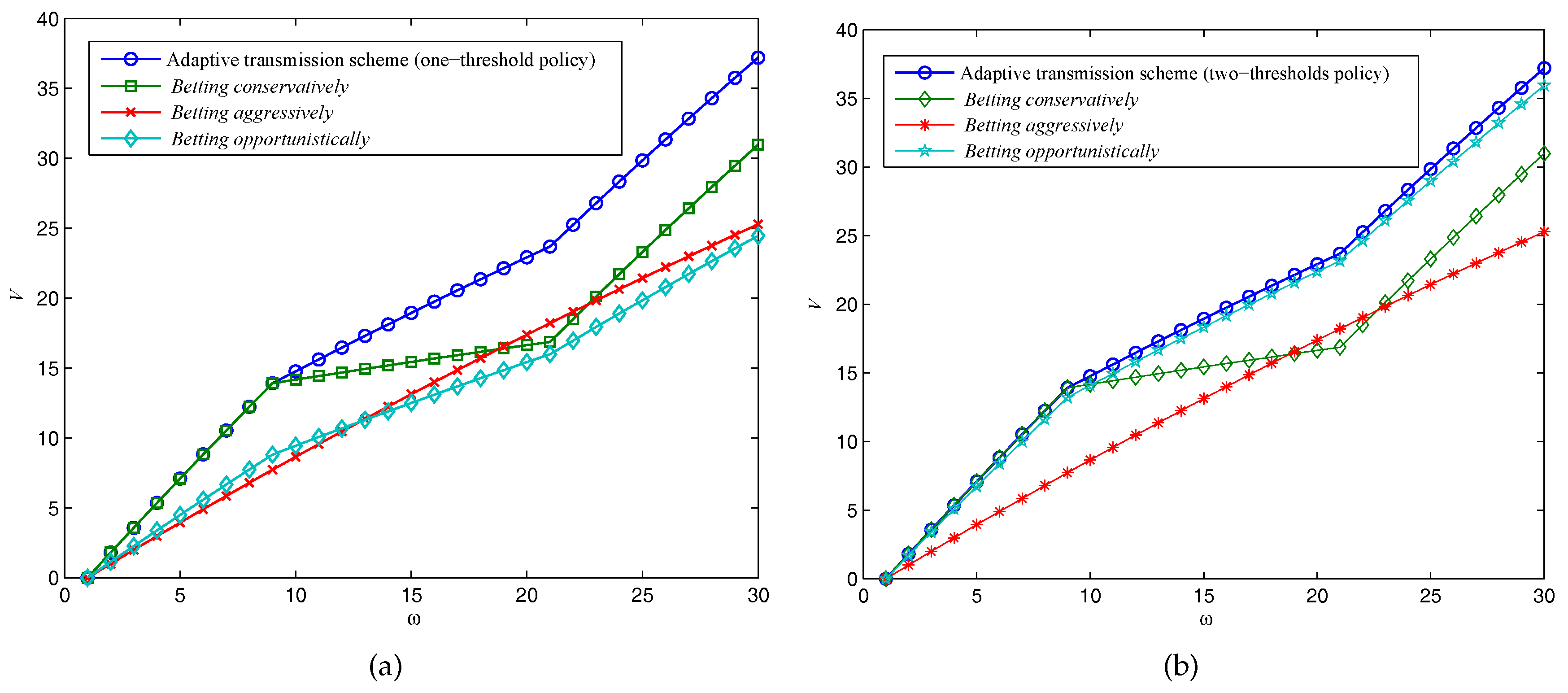
Next, we compare the long-term effect of the expected throughput of our adaptive data transmission scheme with conventional fixed-rate schemes, to validate the optimality of our POMDP-based transmission policy over Ka-band channels for SIN communications. Let w denote the number of the transmission time slots $W=\{w_1,w_2,...,w_n\}$, and $\mathcal{V}={\sum }_{i=1}^w{V}_{\beta }\left(X_i\right)$ denote the accumulated expected values in Figure 6.

The system parameters in these scenarios are as follows: $R_g=2$, $R_b=1$, ${\lambda }_1=0.9$, ${\lambda }_0=0.2$, and $\beta =0.99$. With these parameters, the one-threshold policy is optimal for $\tau \in (0.333,1]$, and beyond these critical values, the two-thresholds policy will become optimal. We have ${\tau }_1=0.4$ in Figure 6a, and ${\tau }_2=0.1$ in Figure 6b, respectively. As expected, at the beginning of several transmission time slots, betting conservatively can archive the same throughput as the adaptive transmission scheme does as is illustrated in Figure 6a. However, the adaptive transmission scheme can better utilize the channel capacity when the Ka-band channel turns it into a good state, which leads to a higher throughput in a long-term program. On the other hand, if the two-thresholds policy is optimal as in Figure 6b, betting opportunistically is also performed well, but still has a gap remaining compared to our adaptive transmission scheme due to the reward from “gamble”, and “play safe” will be better than sensing the channel sometimes.

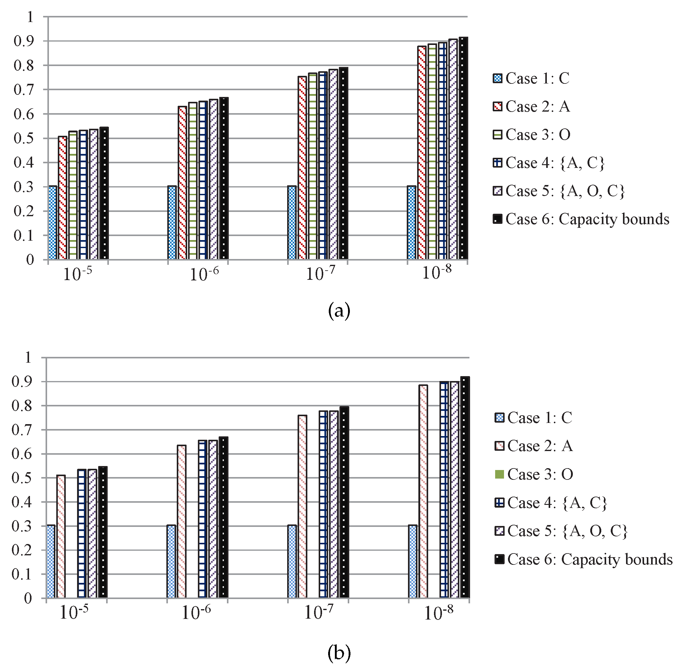
So far, we have demonstrated our POMDP-based transmission policy can perform well with different communication setups. In the following, we simulate and compare the adaptive transmission schemes under Ka-band channel communications.

Assume the threshold of the two-state GE channel noise temperature is $T_{th}=20$ K, and the corresponding transition probability of the GE channel is $\mathbf{G}=\left[\begin{array}{cc}0.9773& 0.0223\\ 0.1667& 0.8333\end{array}\right]$, according to [24]. If the channel state is bad, the channel bit error rate (BER) is ${10}^{-3}$, and we select four different BERs ${10}^{-8}$, ${10}^{-7}$, ${10}^{-6}$ and ${10}^{-5}$ as the channel state is good. Assume normalized the data bit $R_g=1$ when BER is ${10}^{-8}$, then we can calculate data bits $R_b$ and $R_g$ with other BER values according to the error function [24]. We simulate the adaptive transmission schemes in two cases, Earth-to-Moon ($\tau =0.03$), and Earth-to-Mars ($\tau =1$), and the transmission schemes are as follows.

Case 1: The transmitter adopts the action of betting conservatively regardless of the channel state, which can ensure $R_b$ data bits are successfully transmitted.

Case 2: The transmitter only adopts the action of betting aggressively, if the channel state is good, $R_g$ bits are successfully transmitted; else, if the channel state is bad, all data bits are lost.

Case 3: The transmitter only adopts the action of betting opportunistically, if the channel state is good, $(1-\tau )R_g$ bits can be received; else, if the channel state is bad, $(1-\tau )R_b$ bits can be received successfully.

Case 4: The transmitter chooses optimal action by using delayed feedback CSI and and Theorem 2, the adaptive data transmission action space is a, $a\in \{A,C\}$.

Case 5: The transmitter chooses optimal action by using delayed feedback CSI and Theorem 3, the adaptive data transmission action space is a, $a\in \{A,O,C\}$.

Case 6: We directly give the outage capacity bounds of the corresponding channels.

The simulation results of throughput performance of the 5 transmission schemes above and the capacity bounds are shown in Figure 7, and we can see that if the right transmission scheme with certain channel conditions can be selected by using our derived thresholds, it can increase the throughput in Ka-band SIN communications.

Based on the previous analysis, we can expect that the two-thresholds policy is optimal for the Moon-to-Earth scenario in Figure 7a as the sensing cost is $\tau =0.03$. Therefore, the transmitter can access the sensing action with little cost. As it can be seen in Figure 7a, the total number of transmitted bits of betting opportunistically is substantially augmented and the two-thresholds policy transmission scheme performs close to the capacity bounds.

On the other hand, the round trip time between Mars-to-Earth is about 6–40 min, which is leading to the one-threshold policy being optimal with $\tau =1$, and betting opportunistically is completely unfeasible as shown in Figure 7b, there is no data bit that can be transmitted if the transmitter perform channel sensing. And the two-thresholds policy transmission scheme in this scenario is degenerated to the one-threshold policy transmission scheme, where both of the transmission schemes have exactly the same expected total number of transmitted bits.

5. Conclusions

In this paper, considering the potential of the Ka-band high throughput satellites applications to SINs, we reviewed the rain attenuation over Ka-band channel and modeled a two-state Gilbert–Elliot channel for SINs. Then, we proposed an optimal transmission scheme based on POMDP by using the delayed feedback CSI, and derived the thresholds over Ka-band channels for SINs of which we should perform channel sensing or not at the beginning of each transmission time slot. We also derived the thresholds of choosing data transmitting actions from two or three actions in POMDP. Simulation results show that the proposed optimal transmission policy can increase the throughput in SIN communications.