Article

Entropy Generation through Non-Equilibrium Ordered Structures in Corner Flows with Sidewall Mass Injection

by
LaVar King Isaacson
Mechanical Engineering, University of Utah, 2067 Browning Avenue, Salt Lake City, UT 84108, USA
Entropy 2016, 18(8), 279; https://doi.org/10.3390/e18080279
Submission received: 22 June 2016 / Revised: 24 July 2016 / Accepted: 25 July 2016 / Published: 28 July 2016
(This article belongs to the Special Issue Advances in Applied Thermodynamics II)

Abstract

:
Additional entropy generation rates through non-equilibrium ordered structures are predicted for corner flows with sidewall mass injection. Well-defined non-equilibrium ordered structures are predicted at a normalized vertical station of approximately eighteen percent of the boundary-layer thickness. These structures are in addition to the ordered structures previously reported at approximately thirty-eight percent of the boundary layer thickness. The computational procedure is used to determine the entropy generation rate for each spectral velocity component at each of several stream wise stations and for each of several injection velocity values. Application of the procedure to possible thermal system processes is discussed. These results indicate that cooling sidewall mass injection into a horizontal laminar boundary layer may actually increase the heat transfer to the horizontal surface.

Graphical Abstract

1. Introduction

Entropy generation rates for corner flows with sidewall mass injection were reported by the author in a previous article [1]. These computations indicated the generation of non-equilibrium ordered structures at a normalized vertical station of approximately thirty-eight percent of the normalized laminar boundary layer thickness. The present article presents additional computations for entropy generation rates predicted at a normalized vertical station of approximately eighteen percent of the normalized laminar boundary layer thickness for corner flows with a variety of injection mass velocities. The flow configuration considered consists of a corner flow environment, with sidewall mass injection, with the mass injection uniform in the steam wise direction, along the vertical sidewall at the intersection of the sidewall with the horizontal surface. A schematic diagram for this configuration is shown in Figure 1.
The first computational component is the calculation of the steady flow laminar velocity profiles along the horizontal surface in the stream wise-vertical (x-y) plane and the steady flow orthogonal boundary layer profile in the span wise-vertical (z-y) plane. These profiles are computed using the program listings provided by Cebeci and Bradshaw [2] and Cebeci and Cousteix [3]. The similarity characteristics for these orthogonal profiles proved by Hansen [4] justify the simultaneous use of these profiles in our three-dimensional flow configuration.
The next computational component casts the time-dependent spectral equations of Townsend [5] and Hellberg et al. [6] into a Lorenz format (Sparrow [7]) to yield the nonlinear time series solutions for the fluctuating components of the spectral velocity field.
The nonlinear time series solutions of the modified Lorenz equations yield both smooth trajectories and trajectories with fluctuating spectral velocity components within the series. Statistical analysis of the fluctuating spectral time-series solutions yields the entropy generation rates for the given flow configurations. The correspondence of the peaks of the spectral power density analysis and the empirical modes of the singular value decomposition analysis is brought about by the Weiner–Khintchine theorem relating the power density spectrum and the autocorrelation function for the nonlinear time series data [8] (pp. 354–355).
The power spectral densities within the nonlinear time series solutions for the fluctuating spectral velocity components are computed using Burg’s method [9], providing the spectral peaks of the ordered structures within the time series solutions [10] (pp. 572–574). The singular value decomposition method [10] (pp. 59–70) is also used to compute the empirical modes within the same time series, corresponding to the power spectral density peaks found from Burg’s method. These results yield the values for the empirical entropies for the ordered structures as defined by Rissanen [11]. The empirical entropy for each of the modes from the singular value decomposition process yields a corresponding entropic index of the format postulated by Tsallis [12]. Then, from each of these entropic indices, the method of Arimitsu and Arimitsu [13] yields a corresponding value for the intermittency exponent. Combining these computational components into an overall computational procedure, we then compute the entropy generation rate for each of the ordered structures identified in the nonlinear time series solutions of the non-equilibrium spectral equations. The specific computational components are more fully described in Isaacson [1,14]. This article includes the following sections:
In Section 2, the thermodynamic and transport processes of the working substance required for the computational procedures are discussed. In this study, the working substance is the flow of air at a specified temperature and pressure. In Section 3, the mathematical and computational bases for the computation of the steady three-dimensional boundary layer environment are reviewed. In Section 4, the fluctuation equations of Townsend [5] are transformed into the spectral plane and written in the Lorenz format. Section 5 presents computational results for the time-dependent spectral velocity components for various sidewall mass injection velocities at various stream wise locations. Section 6 discusses the extraction of empirical entropies, empirical entropic indices, and intermittency exponents from the nonlinear time series solutions of the modified Lorenz equations. Section 7 presents the results for the computation of the entropy generation rates through ordered structures in the boundary layer environment for various sidewall injection velocities and various stream wise locations. Section 8 includes a comparison of the entropy generation rates for two vertical locations within the laminar boundary layer and compares these values with the entropy generated in a corresponding turbulent boundary layer. The article closes with a discussion of the results and final conclusions.

2. Selection of Heated Air as the Working Substance

The flow configuration we are simulating in this exploratory study is shown in Figure 1. The figure is intended to represent the corner flow in the entrance to a square channel in, for example, an industrial heating unit. In this section, we describe the characteristics of the working gas we use in our computational procedure.
The working gas is assumed to be heated air with the following thermodynamic and transport properties:
Air temperature, T: 1068.0 K
Static pressure, p: 0.912 × 10⁵ N/m2
Kinematic viscosity, ν: 1.51634 × 10⁻⁴ m2/s
It should be noted that the value for the kinematic viscosity used in this study is very similar to the values used in previous studies. The explanation for this is that a series of coupled, nonlinear time-dependent differential equations are included in the computational procedure. The solutions for such equations are very sensitive to the initial conditions imposed on the equations and are also sensitive to the control parameters applied in the solution. The solution of the steady-state boundary-layer equations that provides these control parameters is dependent on the particular value of the kinematic viscosity applied in the calculations. We have found that only a narrow range of kinematic viscosities yields the prediction of ordered structures from the computational procedure [1]. The choice of air at the given temperature and pressure yields an appropriate value for the kinematic viscosity. The range of appropriate values of kinematic viscosities has not been delineated and remains as work to be done.
A fundamental feature of the computational procedure discussed in this article is the embedding of the time-dependent Lorenz-format equations in the reservoir of steady-state boundary layer velocity gradients obtained from the time independent boundary layer equations.
To clarify the essential nature of this feature, the next section presents a summary of the mathematical and computational methods used for the determination of the reservoir steady-state laminar boundary-layer velocity gradients. These boundary layer mean velocity gradients are time independent but vary with the stream wise distance x. The mean velocity gradients serve as control parameters for the time-dependent initiation of instabilities within the boundary layer for each stream wise station, as summarized in Section 4 of the article.

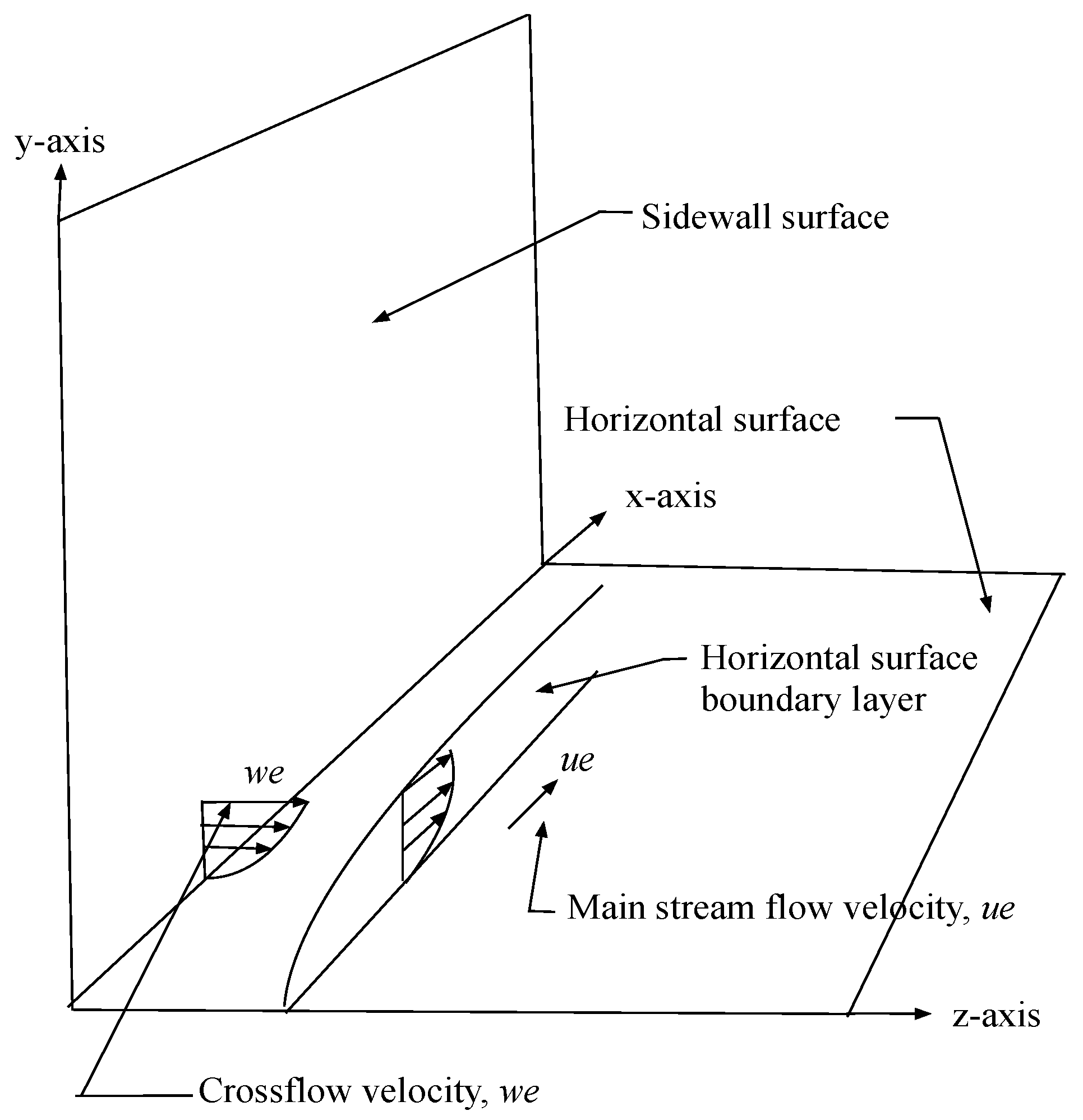
3. Steady-Flow Laminar Boundary-Layer Environment

The boundary-layer configuration considered in this article consists of a laminar boundary layer in the x-y plane produced by the stream wise velocity along the horizontal surface and a laminar boundary layer in the z-y plane produced by mass injection from the sidewall in the z-direction. The momentum equation for the thin-shear boundary layer approximation may be written ([2], pp. 39–45) as:
u u x + v u y = 1 ρ d p d x + 1 ρ y [ μ u y ρ u v ¯ ] .
The boundary conditions for Equation (4) are:
y = 0 ,   u = v = 0 ,
y = δ ( x ) ,   u = u e ( x ) .
The Reynolds shear stress for the computation of turbulent boundary layers is modeled with the “eddy viscosity”, ε m , having the dimensions of (viscosity)/(density), by:
ρ u v ¯ = ρ ε m u y .
The computer program we have chosen to implement for the solution of the boundary layer equation (Equation (4)) is based on the Keller–Cebeci box method presented by Cebeci and Bradshaw [2] and Cebeci and Cousteix [3]. One of the basic aspects of this method is to transform Equation (4) into a system of first-order ordinary differential equations. The Falkner–Skan transformation, in the form:
η = ( u e ν x ) 1 / 2 y ,
is introduced into the transformation process. The dimensionless stream function, f ( x , η ) , is defined by:
Ψ ( x , y ) = ( u e ν x ) 1 / 2 f ( x , η ) .
These definitions yield the results for the mean boundary layer velocities u and v as:
u = u e f ,   v = x [ ( u e ν x ) 1 / 2 f ] + η 2 ( u e ν x ) 1 / 2 f .
Differentiation with respect to η is indicated by the prime in these expressions.
From Bernoulli’s equation, the pressure gradient term is given by d p d x = ρ u e d u e d x . To simplify the resulting equations, the parameter m is defined as:
m = x u e d u e d x .
Through the application of the transformation process, (we refer the reader to Cebeci and Bradshaw [2] for the details) the basic partial differential equation for the boundary layer (Equation (4)) is replaced with three first-order partial nonlinear differential equations in the following form:
f = u ,
u = v ,
( b v ) + ( m + 1 2 ) f v + m ( 1 u 2 ) = x ( u u x v f x ) .
In Equation (14), b = ( 1 + ε m + ) and ε m + = ε m ν . The corresponding boundary conditions for Equations (12)–(14) are:
f(x, 0) = 0, u(x, 0) = 0, u(x, η) = 1
Note that in Equation (13), v is not the y-component velocity.
Cebeci and Bradshaw [2] present computer program listings for the numerical solutions for both laminar and turbulent boundary layers over flat plate surfaces. The program listings used in the study reported here are those presented in [2].
Hansen [4] has indicated that orthogonal laminar boundary layer profiles in a three-dimensional coordinate system possess the characteristic of similarity. We therefore use the boundary layer computations for both the profiles in the x-y plane and in the z-y plane. The steady state boundary layer equations and the corresponding velocity gradients serve as the thermodynamic steady state reservoir that provides the control parameters for the time-dependent development of the spectral fluctuations within the boundary layer environment [8] (pp. 26–31).

4. Modified Time-Dependent Lorenz Equations in the Spectral Plane

4.1. Transformation of the Townsend Equations to the Modified Lorenz Format

The crosswind velocity of the mass injected in the z-direction from the sidewall produces a laminar boundary layer along the horizontal surface in the z-y plane. This boundary layer is orthogonal to the laminar boundary layer in the x-y plane. The nonlinear interactions of this z-y boundary layer within the laminar boundary layer in the x-y plane generate instabilities within the three-dimensional laminar boundary layer flow. The methods of Townsend [5] are used to obtain a set of non-equilibrium, time-dependent equations in the spectral domain for these non-equilibrium instabilities, separate from the equations for the steady boundary layer flow.
Separating the equations of motion into steady and unsteady equations, the equations for the velocity fluctuations may then be written as [5,6]:
u i t + U j u i x j + u j U i x j + u j u i x j = 1 ρ p x i + ν 2 u i u j u j .
In these equations, ρ is the density and ν is the kinematic viscosity, Ui represent the mean boundary layer velocity components with i = 1, 2, 3 indicating the x, y, and z components, and xj, with j = 1, 2, 3, designate the x, y and z directions. The pressure term is eliminated by taking the divergence of Equation (16) and invoking incompressibility, yielding:
1 ρ 2 p x l 2 = 2 U l x m u m x l + u l x m u m x l .
We wish to transform these equations into the spectral plane for the computational solutions for the time-dependent fluctuating spectral components. The solutions of the spectral equations yield the spectral wave vector components and the spectral velocity wave components. Through Parseval’s theorem, the products of the spectral velocity components represent the products of the fluctuating velocity components in the physical plane. The statistical analysis of the spectral velocity component time series solutions then yields the entropy generation rates within the boundary layer non-equilibrium ordered structures.
The fluctuating velocity and pressure fields of Equations (16) and (17) may be expanded in terms of the Fourier components (Mathieu and Scott [15]) as:
u i ( x , t ) = k a i ( k , t ) exp ( i k x )
and:
p ( x , t ) ρ = k b ( k , t ) exp ( i k x ) .
The pressure component in Equation (16) is transformed into a function of spectral velocity components and boundary layer velocity gradients through Equations (17) and (19). Substituting the resulting equations and Equation (18) into Equation (16) yields an expression for the fluctuations of the spectral components with time. The equations for the time-dependent three spectral velocity wave components, ai(k), are then given as:
d a i ( k ) d t = ν k 2 a i ( k ) U i x i a i ( k ) + 2 k i k l k 2 U l x m a i ( k ) + i k + k = k ( k l k i k m k 2 δ i m k l ) a l ( k ) a m ( k ) .
The general equations for the balance of transferable properties give the equations for the spectral wave numbers, ki as:
d k i d t = U l x i k l .
The set of equations for the time-dependent wave number components, including the gradients of the mean velocities in the x-y and z-y boundary layers, may be written:
d k x d t = U x k x V x x k y ,
d k y d t = U y k x V x y k y W y k z ,
d k z d t = V z z k y W z k z .
The nonlinear products of the spectral velocity components in Equations (20) are retained in our series of equations by characterizing the coefficients:
k l ( δ i m k i k m k 2 )
as a projection matrix [15]. This coefficient represents the projection of a given velocity wave vector component, ai, normal to the direction of the corresponding wave number component, ki. A model equation for this expression in the form:
1 − K·cos(k(t))
is introduced to retain the effect of the projection matrix on the nonlinear interactive terms in our equations. K is an empirical weighting amplitude factor [14] and k(t) is given by:
k ( t ) = ( k x 2 ) .
With F = Kcos(k(t)), the equations for the spectral velocity components, Equations (20), are written in Lorenz format as [14]:
d a x d t = σ y a y σ x a x ,
d a y d t = ( 1 F ) a x a z + r 1 a x s 1 a y ,
d a z d t = ( 1 F ) a x a y b 1 a z .
From Equations (20), the coefficients of the velocity wave component terms have the following forms [14]:
σ y = [ ( 2 k x k y k 2 1 ) U y + 2 k x k y k 2 V x y + 2 k x k z k 2 W y ] ,
σ x = { υ k 2 [ ( 2 k x k x k 2 1 ) U x + 2 k x k y k 2 V x x + 2 k x k z k 2 W x ] } ,
r 1 = [ 2 k y k x k 2 U x + ( 2 k y k y k 2 1 ) V x x + 2 k y k z k 2 W x ] ,
s 1 = { υ k 2 [ 2 k y k x k 2 U y + ( 2 k y k y k 2 1 ) V z y + 2 k y k z k 2 W y ] } ,
b 1 = { υ k 2 [ 2 k z k x k 2 U z + 2 k z k y k 2 V z z + ( 2 k z k z k 2 1 ) W z ] } .
The nonlinear time series solutions for the spectral velocity wave number components in the spectral domain for each of the seven downstream stations make up the non-equilibrium thermodynamic system. Solutions of the overall set of equations are obtained at each of the seven stations along the x-axis.
The application of these equations at the initial station requires that additional assumptions be applied to the modified Lorenz equations. Isaacson [14], Mathieu and Scott [15], and Manneville [16] have discussed both the format and justification for the particular choice of these assumptions for the initial station. These solutions contain the spectral velocity component fluctuations that we wish to study.
We apply our computational procedure to the six stations following the initial station at x = 0.08 along the stream wise direction. However, as Attard [8] (pp. 42–45) points out, we must take into account that the nonlinear time series solutions obtained for the second and subsequent stations will be influenced by the fluctuations produced in the first and following stations. To accomplish this, we use the synchronization properties of the modified Lorenz set of equations describing the nonlinear solutions for the spectral components [1,14].

4.2. Synchronization Properties of the Modified Lorenz Equations

Pecora and Carroll [17], Pérez and Cerdeiral [18], and Cuomo and Oppenheim [19] have used the synchronization properties of systems of Lorenz-type equations to extract messages masked by chaotic signals. The synchronization properties of Lorenz-type equations are adapted here to extract ordered signals from the nonlinear time series generated for each of the spectral components in the solutions of the modified Lorenz equations.
As indicated previously, the solutions are obtained for a sequence of stations along the x-axis. We apply the transformation of the projection matrix (Equation (26)) to the initial station at x = 0.080. We then apply the synchronization properties to each of the following downstream stations. The various boundary layer coefficients at each of these stations are computed in the same manner as in the initial station. Following the results in [14], the time-dependent output for the x-direction spectral velocity component from the initial station is used as input to the nonlinear coupled terms in the modified Lorenz equations at the next station, which we denote as the second station in the x-direction. Then, the input to the nonlinear-coupled terms at the next downstream station is made up of the sum of the stream wise velocity wave component output from the initial station plus the x-direction spectral velocity wave component output from the next downstream station. This process is repeated for each of the six downstream stations. With this method, the memory of the initial velocity fluctuations and the influence of subsequent fluctuations are retained in the overall computational procedure.

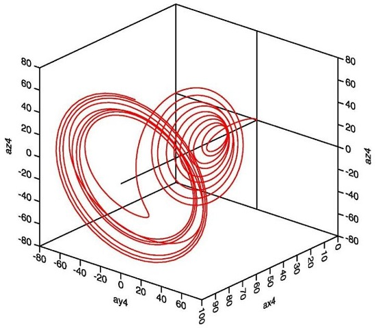
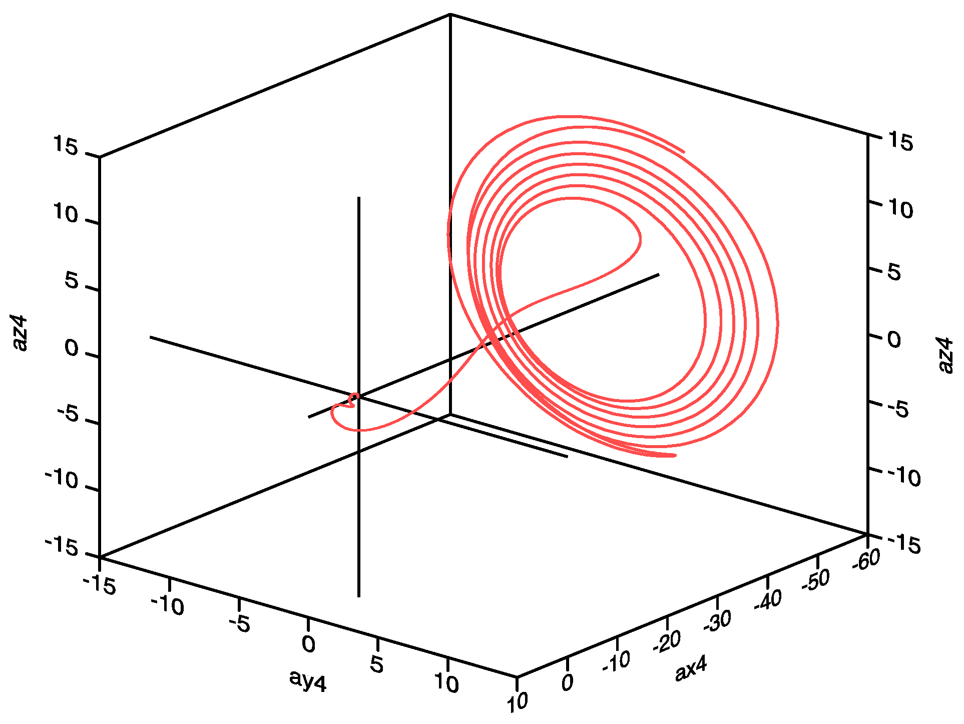
4.3. Deterministic Results for the Modified Lorenz Equations

The stream wise velocity has been chosen as ue = 1.00 for all of the cases considered in this study. We have chosen to present the results obtained at the station of x = 0.140 since the results for this station indicate the clearest power spectral density peaks in the overall set of statistical results. However, it turns out that the results for this station also indicate the lowest level of entropy generation rates at the normalized boundary layer location of η = 1.40 for the crosswind velocity of we = 0.0800. This choice for the presentation of the results should therefore be kept in mind in the comparison of entropy generation rates for the overall set of crosswind velocities.
Figure 2 presents the deterministic three-dimensional spectral velocity wave trajectory for the downstream station of x = 0.140, for a sidewall mass injection velocity of we = 0.0800. Figure 3 shows the corresponding phase diagram for az4ay4, where ay4 is the normal spectral velocity wave component and az4 is the span wise spectral velocity wave component, again at the station x = 0.140.
Figure 4 presents the deterministic three-dimensional trajectory of the spectral velocity wave components for the downstream station of x = 0.140, for a sidewall mass injection rate of we = 0.0925. Figure 5 shows the corresponding phase diagram for az4ay4, where ay4 is the normal spectral velocity wave component and az4 is the span wise spectral velocity wave component, again at the station x = 0.140 and crosswind velocity of we = 0.0925.

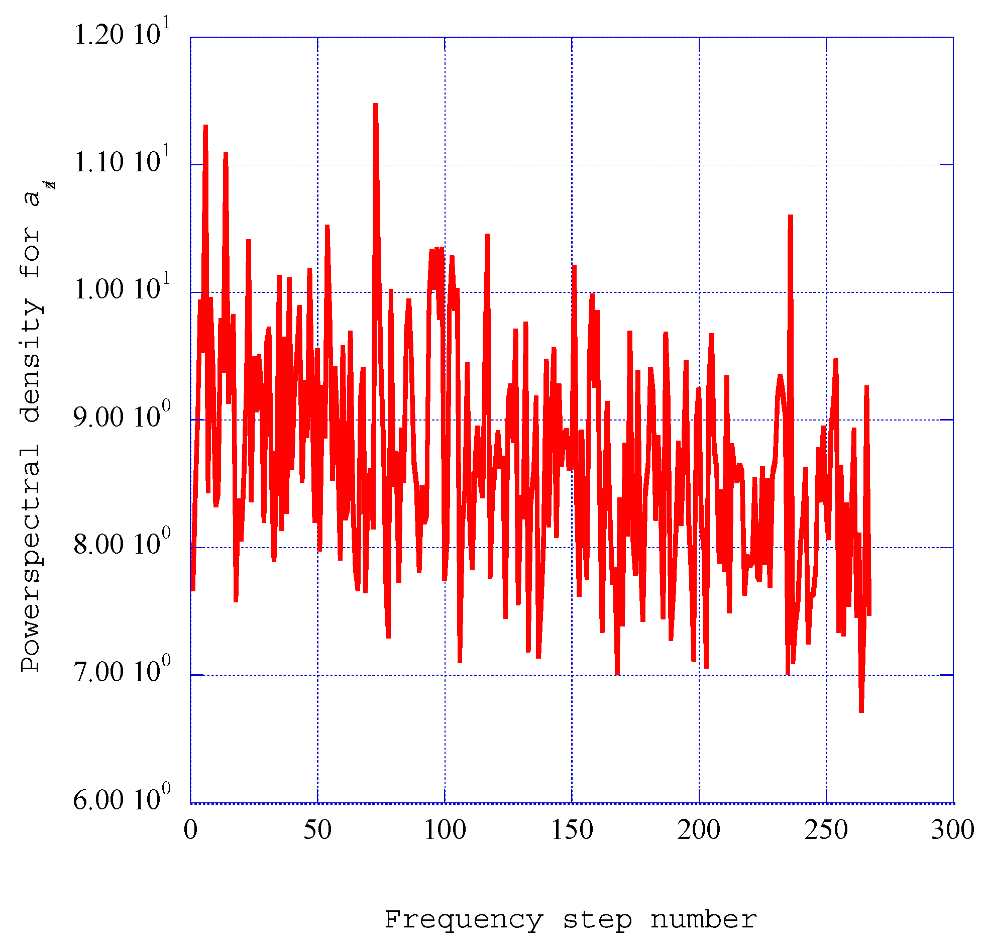
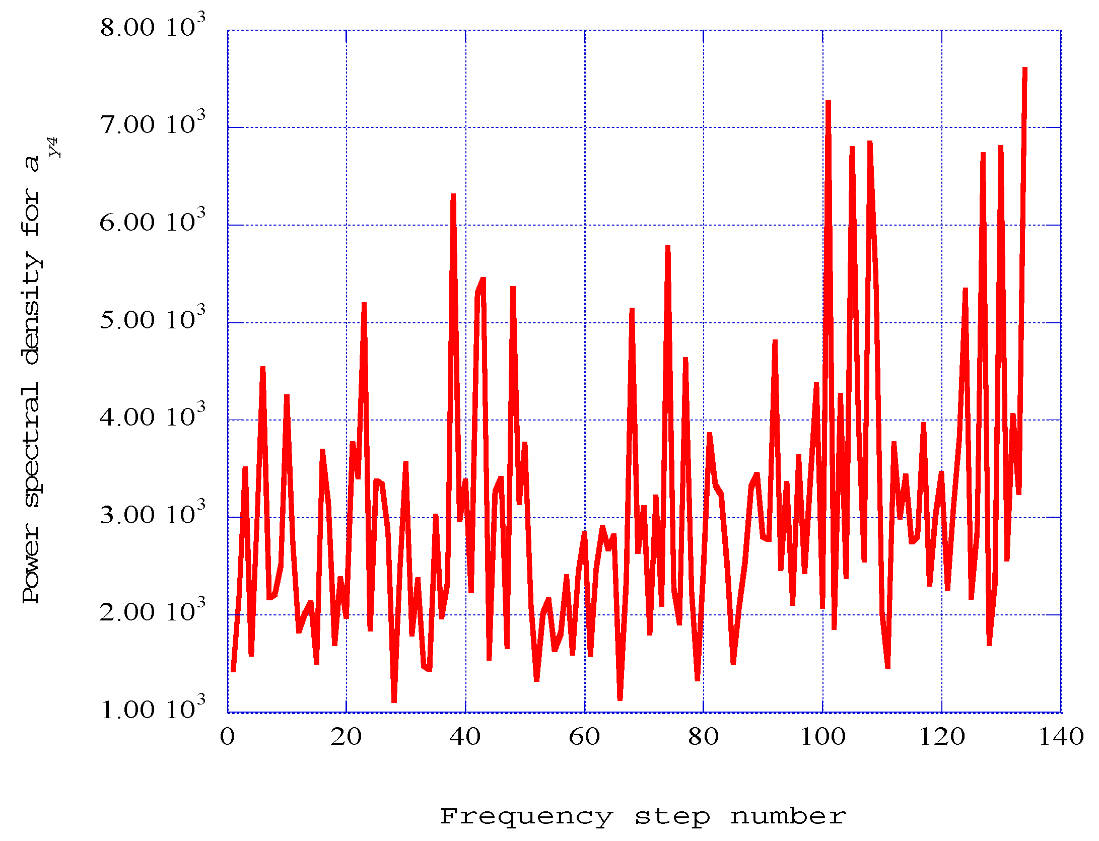
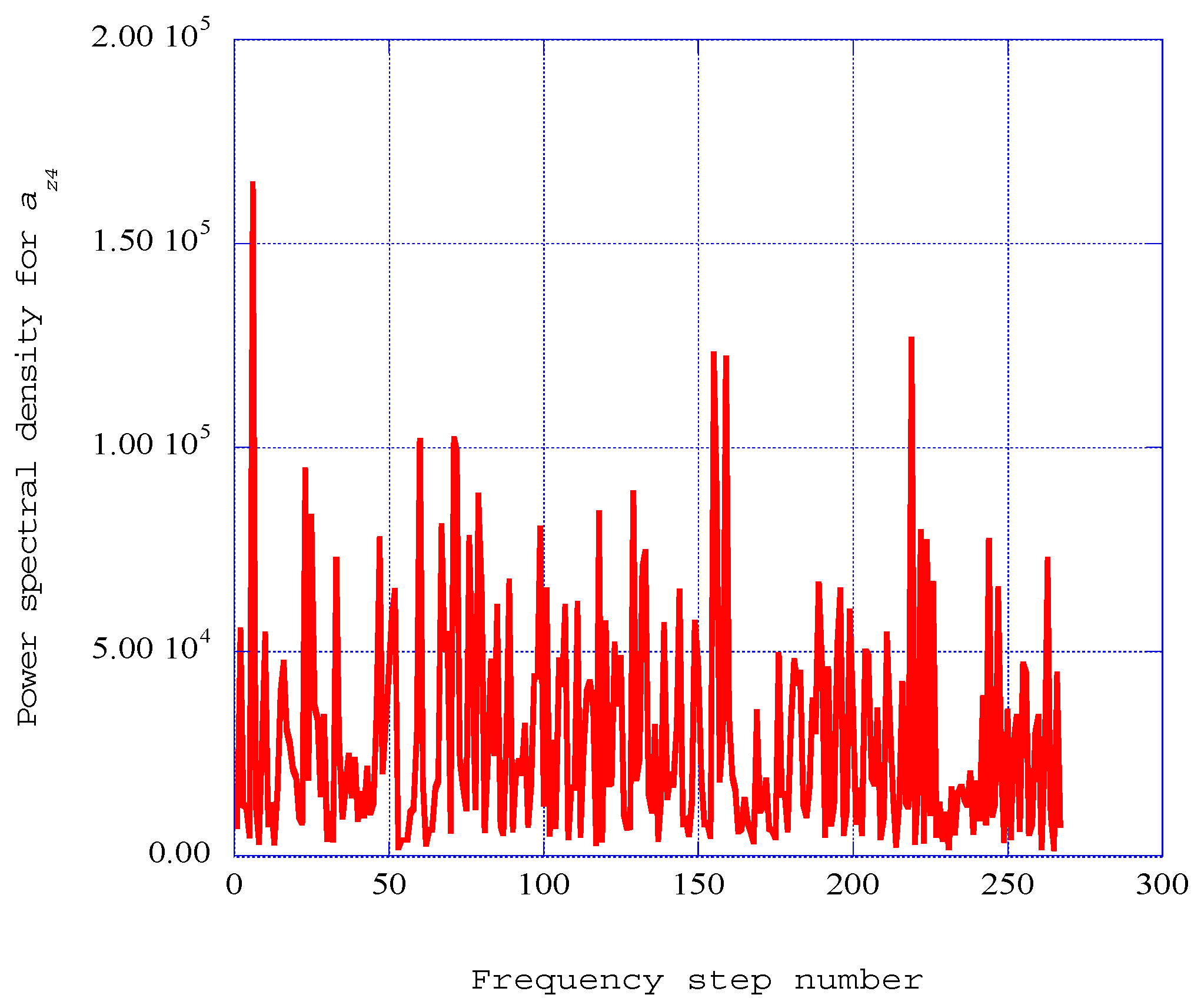
5. Power Spectral Density within the Non-Equilibrium Spectral Velocity Fluctuations

5.1. Power Spectral Densities Indicating Ordered Structures

The Lorenz synchronization procedure yields the nonlinear time series solution for each of the six stations in the x-direction, following the initial station. These solutions indicate the generation of deterministic spiral structures, with significant non-equilibrium velocity fluctuations embedded within some of the solutions. Entropy generation comes about through the dissipation of these fluctuations into equilibrium thermodynamic states. We have found that Burg’s method [9] for the power spectral density of the time-series data is an effective method for extracting the underlying structural characteristics of the velocity fluctuations within the nonlinear time series solutions.
The resulting power spectral density results for the normal spectral velocity wave component, ay4 at the fourth station at x = 0.140, are presented in Figure 6. For each of the power spectral density results, we have assigned empirical mode numbers to these peaks, starting with mode j = 1 representing the highest peak in the distribution, continuing to mode j = 16, representing the corresponding lowest peak among the sixteen peaks.
The peaks of the spectral power density analysis and the empirical modes of the singular value decomposition analysis are computed from the same set of time series data. Therefore, we can relate each power spectral density peak with a corresponding empirical mode through the Weiner−Khintchine theorem relating the power density spectrum and the autocorrelation function for the nonlinear time series data [8] (pp. 354–355).
The resulting power spectral density results for the span wise spectral velocity wave component, ay4 at the fourth station at x = 0.140, are presented in Figure 7.
The power spectral density results for the normal spectral velocity wave component, ay4 at the fourth station at x = 0.140 for a crosswind velocity of we = 0.0925, are presented in Figure 8. The resulting power spectral density results for the span wise spectral velocity wave component, ay4 at the station at x = 0.140, for a crosswind velocity of we = 0.0925, are presented in Figure 9.
A significant advantage of Burg’s method (the maximum entropy method) is the enhancement of the spectral peaks in the power spectral density distribution. Press et al. [10] (pp. 572–575) present computer program listings for the prediction of the power spectral density using the maximum entropy method. The results indicate that the power spectral density is distributed over a selection of well-defined spectral peaks. These spectral peaks represent a collection of ordered structures embedded within the fluctuating time series solutions of the modified Lorenz equations, each identified with a corresponding mode number.
These spectral peaks have been organized in descending order into sixteen empirical modes. Simpson’s integration rule is used to obtain the kinetic energy available for dissipation for each of the power spectral density modes. The total spectral energy available for dissipation is then obtained as the sum of the individual contributions across the modes. This value is then used to get the fraction of dissipation energy in each mode that is eventually available for dissipation into the internal energy of the final equilibrium thermodynamic state.

5.2. Empirical Entropies from Singular Value Decomposition

The singular value decomposition procedure [20] can also serve as a means of identifying fundamental characteristics of the nonlinear time series solutions of the coupled nonlinear spectral equations. We have incorporated into our numerical procedure the singular value decomposition computer program listings presented by Press et al. [10] (pp. 59–65). The computational procedure is made up of two parts, the computation of the autocorrelation matrix and the singular value decomposition of that matrix [10]. The overall computational procedure yields the empirical eigenvalues for each of the empirical eigenfunctions for the given nonlinear time series data segment.
The application of the singular value decomposition procedure to a specified segment of the nonlinear time-series solution for each of the spectral velocity wave components yields the distribution of the component eigenvalues λ j across the empirical modes, j, for the flow conditions listed in Equations (1)–(3). The empirical entropy, Sempj, is defined from these eigenvalues by the expression [11]:
S e m p j = ln ( λ j ) .
Here, λj is the empirical eigenvalue computed from the singular value decomposition procedure applied to the nonlinear time-series solution. The distribution of the empirical entropy across the decomposition empirical modes has been shown in [14]. We have applied the singular value decomposition procedure to the nonlinear time-series solutions of the modified Lorenz non-equilibrium equations. Again, invoking Parseval’s formula [14], the empirical eigenvalues produced by the singular value decomposition procedure represent twice the kinetic energy associated with the fluctuating velocity fields [20].

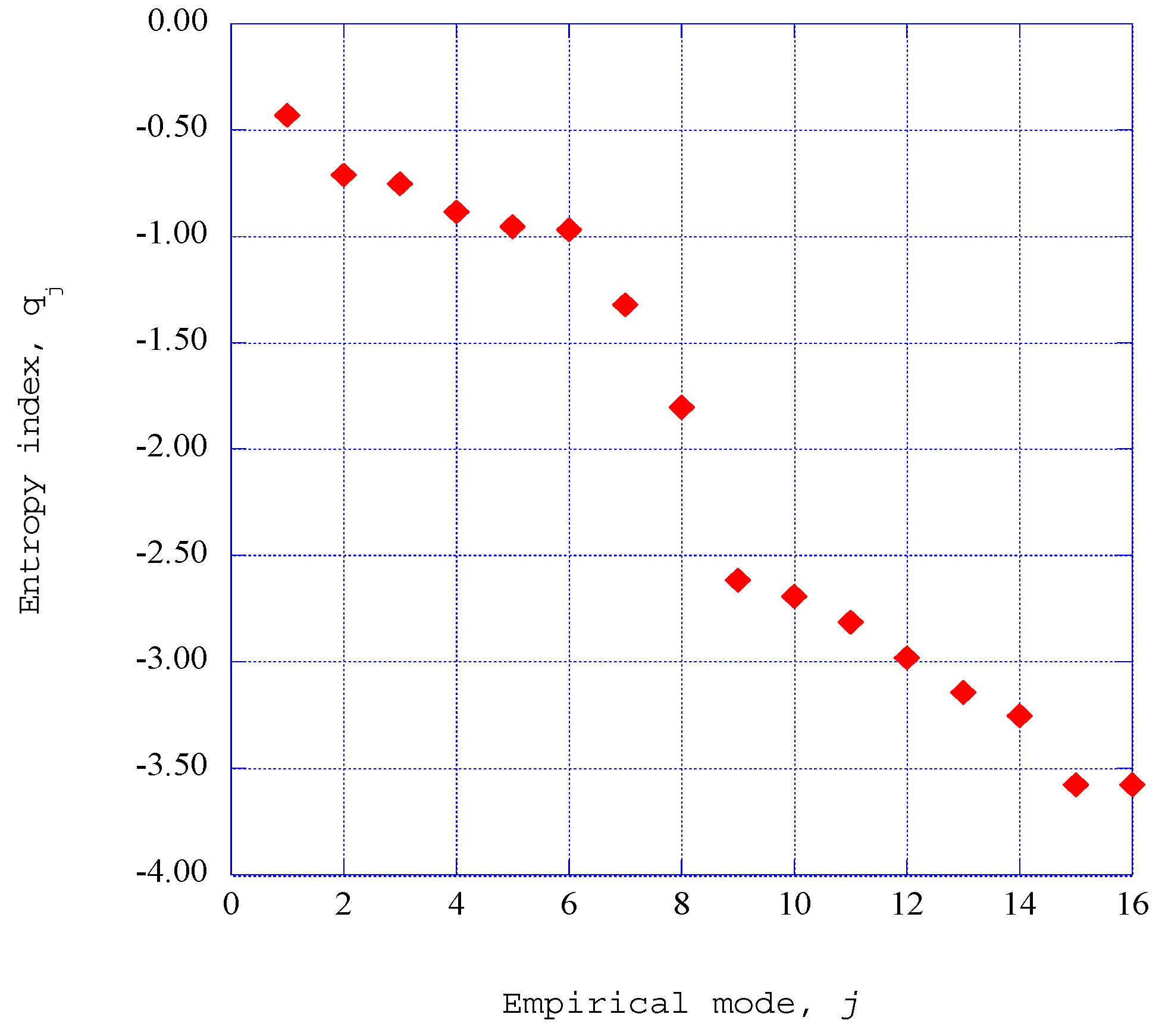
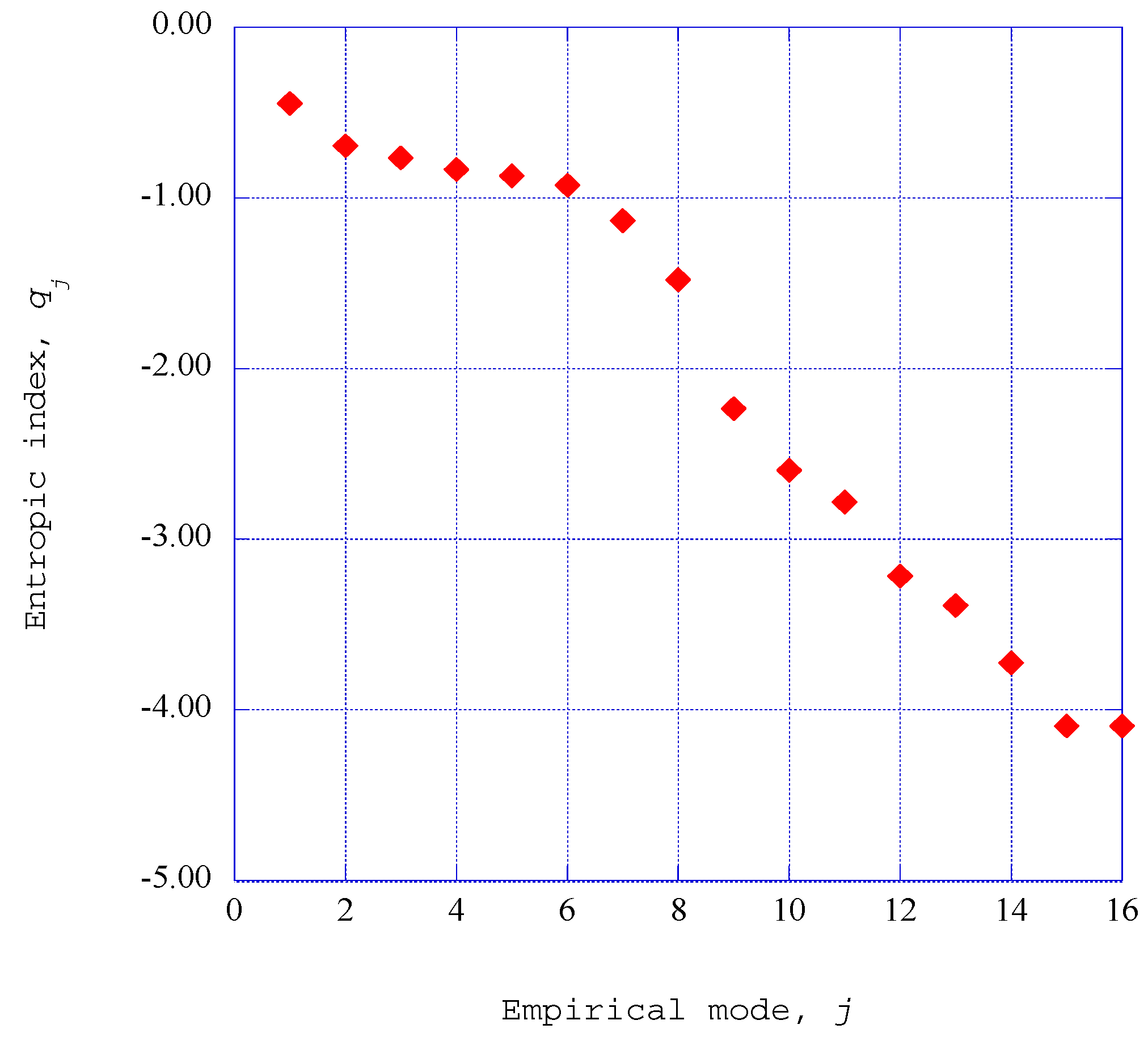
5.3. Empirical Entropic Indices for the Ordered Structures

The empirical entropies for the fluctuating spectral velocity wave component time series indicate different characteristics for the various non-equilibrium collections embedded within the time series. These results indicate that the majority of the kinetic energy is contained within the first six empirical modes of the singular value decompositions, with relatively low empirical entropy. The following three empirical modes indicate a transition into non-equilibrium ordered structures. These structures have been classified as coherent [20] with well-defined structural boundaries. We wish to find a way to follow these structures through the process of transition from ordered structures into equilibrium thermodynamic states. For this, we turn to the concept of the Tsallis entropic format (Tsallis [12]).
The Tsallis entropic format is applicable to a variety of microscopic and macroscopic sub-systems. We are working with a collection of statistical sub-systems spread over a limited number of empirical modes, j. Note that this is not a sequence over time, but is a sequence in phase space [8] (pp. 409–412). The empirical entropy, Sempj is introduced to describe the entropy of an ordered structure described by the empirical eigenvalue, λ j , for the singular value decomposition empirical mode, j. Hence, we simply adopt, in an ad hoc fashion, an expression from which we may extract an empirical entropic index, qj, from the empirical entropy, Sempj. This expression is written as [14]:
S e m p j = ln ( λ j ) = 1 ( λ j ) q j ( q j 1 ) .
This expression includes the effects of the nonlinear, non-equilibrium nature of the ordered structures we are following. It has the format of an entropic index; hence, we simply call qj the empirical entropic index or simply entropic index. The empirical entropic indices for the normal spectral velocity wave component, ay4 at the fourth station at x = 0.140, with a crosswind velocity of we = 0.08000 are presented as a function of the empirical mode j in Figure 10. The empirical entropic indices for the normal spectral velocity wave component, ay4 at the fourth stream wise station at x = 0.140, and a crosswind velocity of 0.0925 are presented as a function of the empirical mode, j in Figure 11.

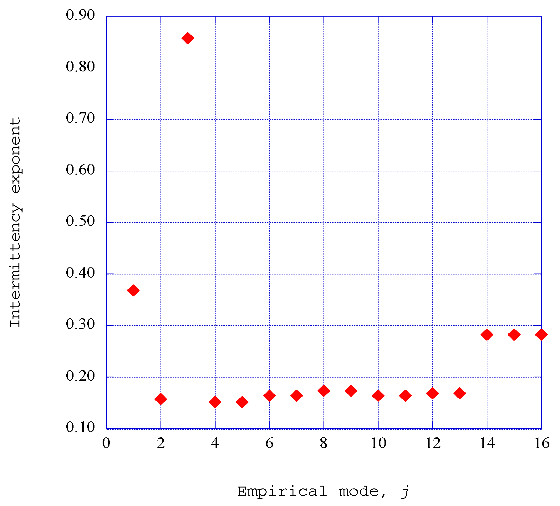
5.4. Empirical Intermittency Exponents for the Ordered Structures

In this section, we introduce a heuristic method to connect the non-equilibrium results for the entropic indices with the final phase of the dissipation of fluctuating kinetic energy into thermodynamic internal energy. We explore this computational connection through the concept of intermittency exponents and a relaxation process into the final thermodynamic entropy state.
The non-equilibrium ordered structures discussed in previous sections are of a macroscopic nature embedded within the nonlinear time series solutions of the nonlinear equations for the fluctuating spectral velocity wave field. Singular value decomposition of the time series solutions provides empirical entropies for these non-equilibrium structures. The empirical entropic indices of the Tsallis form extracted from the empirical entropies using Equation (37) have been used to obtain the intermittency exponents for the ordered structures. We heuristically apply a relationship, found by Arimitsu and Arimitsu [13], connecting the entropic index of Tsallis to the intermittency exponent, ζj. This intermittency exponent describes the fraction of fluctuating kinetic energy within the non-equilibrium ordered structure that is dissipated into thermodynamic internal energy [13].
We will substitute the absolute value of the empirical entropic index discussed in the previous section into the original equation derived by Arimitsu and Arimitsu [13]. This expression is written as:
| q j | = 1 1 + ζ j log 2 ( 1 + 1 2 ζ j ) log 2 ( 1 1 2 ζ j ) log 2 ( 1 + 1 2 ζ j ) log 2 ( 1 1 2 ζ j )
Figure 12 shows the results for the intermittency exponents obtained from Equation (38) for the stream wise location of x = 0.140 with a crosswind velocity of we = 0.0800. These results indicate a dominant intermittency exponent at empirical mode j = 3 and intermittency exponents for the remaining empirical modes close to the observed value of 0.24 [13]. The intermittency exponents for the stream wise location of x = 0.140 with a crosswind velocity of we = 0.0925 are shown in Figure 13. These results again indicate a dominant intermittency exponent at empirical mode j = 3 and intermittency exponents for the remaining empirical modes close to the observed value of 0.24 [13].

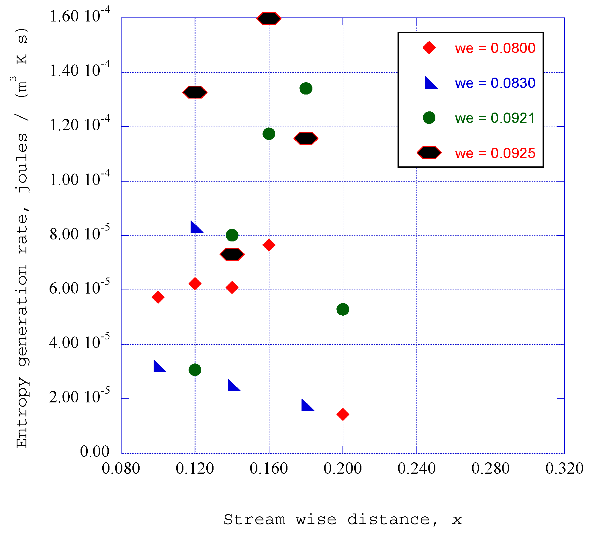
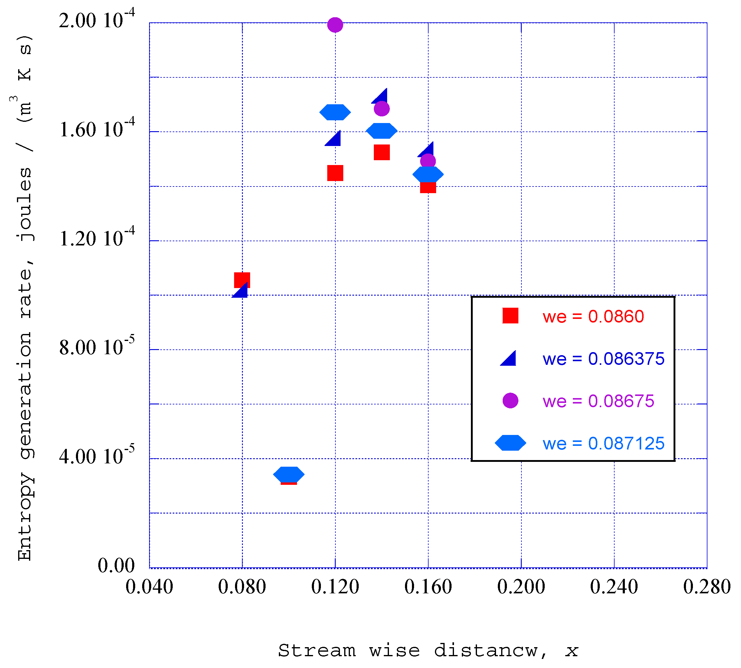
6. Entropy Generation Rates through the Ordered Structures

6.1. Kinetic Energy Available for Dissipation

The local mean flow kinetic energy, u2/2, at the normalized vertical distance, η = 1.40 in the x-y plane boundary layer, is considered as the source of kinetic energy to be dissipated through the spiral structures. This available kinetic energy is distributed over the stream wise component, the normal component and the span wise component. The fraction of kinetic energy in the x-direction velocity component is denoted as κ x , the fraction of kinetic energy in the y-direction velocity component is denoted as κ y in the z-direction velocity component denoted as κ z . The fraction of dissipation kinetic energy within each empirical mode of the power spectral energy distribution is denoted as ξj. Then the total rate of dissipation of the available fluctuating kinetic energy for the stream wise, normal and span wise velocity components is the summation, over the empirical modes, j, of the product of the kinetic energy fraction of each mode times the intermittency exponent for that mode, ζj [1].
The empirical intermittency exponent for each of the empirical modes within the ordered structures has been extracted from the empirical expression (Equation (38)) given by Arimitsu and Arimitsu [13]. At this point in the computational procedure, values are available for the input energy source for the non-equilibrium ordered structures, the fraction of the fluctuation kinetic energy available in each of the empirical modes within the non-equilibrium ordered structures, and the fraction of the energy in each of the empirical modes that dissipates into background thermal energy, thus increasing the thermodynamic entropy. We consider the dissipation process for the ordered structures as a general relaxation process and use concepts from non-equilibrium thermodynamics to describe this dissipation process.

6.2. Entropy Generation Rates for Relaxation Processes

From the concepts of non-equilibrium thermodynamics, de Groot and Mazur [21] (pp. 221–230) write the equation for the entropy generation rate in an internal relaxation process as:
s t = J ( x ) ρ T μ ( x ) x .
Here, s is the entropy per unit mass, ρ is the density, T is the temperature, μ is the mechanical potential for the transport of the ordered structures in an external context and J(x) is the flux of dissipation energy through the ordered structures available for dissipation into thermal internal energy.
The dissipation of the ordered structures into background thermal energy may be considered as a two-stage process from the transition of the ordered structures into equilibrium thermodynamic states and a relaxation process of the downstream velocity in the initial state to the final equilibrium state of the velocity over the internal distance x. At the final equilibrium state, the dissipated ordered structure vanishes into thermal equilibrium with the reservoir. The local boundary layer steady state velocity is written as u = ue f’, where f” is the derivative of the Falkner–Skan stream function f with respect to the normalized distance η. The expression for the entropy generation rate (in J/(m3·K·s)) through the non-equilibrium ordered structures is then written as [1]:
S g e n = ρ [ ( 1 2 u e 2 T ) ( f ) 2 { κ x ( j = 1 16 ξ j ζ j ) x + κ y ( j = 1 16 ξ j ζ j ) y + κ z ( j = 1 16 ξ j ζ j ) z } ( u e x ) ] .
In this expression, ρ is the density of the working substance, in this case air at the given pressure and temperature. The first two terms within the brackets in Equation (40) represent the source of total kinetic energy available from the local steady boundary layer velocity in the stream wise direction. The first factor in each of the three terms within the braces represents the fraction within each of the velocity components of the total kinetic energy from the boundary layer. The first factor in each of the summation terms represents the fraction of kinetic energy within the given spectral mode from the power spectral density distribution. The second factor in each summation is the corresponding intermittency exponent obtained from the empirical entropic index for that mode. The final factor within the brackets is the overall mechanical turnover rate that transports the ordered structures in the given flow environment.
The kinetic energy in each spectral mode available for final dissipation into equilibrium internal energy is computed for each of the spectral peaks. The empirical entropy for each of the structures indicated by the spectral peaks is found from the singular value decomposition process applied to the given time series data segment. The connecting parameter, the empirical entropic index, is then extracted from the resulting value of the empirical entropy.
Glandsdorff and Prigogine [22] find that for the general evolution criterion for non-equilibrium processes, dSempj/dt < 0. When the Tsallis entropic index is negative, Mariz [23] found that the empirical entropy change is also negative, dSempj/dt < 0. The results presented in Figure 10 and Figure 11 indicate that significant non-equilibrium structures exist within the specified time frame of the particular nonlinear time series solution. These regions may therefore be classified as ordered, non-equilibrium structures. Therefore, the significant negative nature for the extracted empirical entropic indices at the fourth station at x = 0.140 is in agreement with both the Prigogine criterion and the Mariz results for the Tsallis entropic index. The ad hoc introduction of an empirical entropy index thus provides a representation of the nonlinear, non-equilibrium ordered structures in a significant way.
Given the absolute value of the empirical entropic index, qj, the intermittency exponent, ζj for the mode, j, is extracted from Equation (38) [13] by the use of Brent’s method [10] (pp. 397–405).
We consider the entropy generation rate to be a phase transition of the dissipation of the non-equilibrium ordered structure into background thermal energy and a relaxation process of the global mechanical transport process of the stream wise velocity, ue over the distance x. At the final equilibrium state, the stream wise velocity of the dissipated structure vanishes. The entropy generation rates through the non-equilibrium ordered structures are then determined from Equation (40) [1].
The entropy generation rates as a function of the downstream stations are shown in Figure 14, with the four values of sidewall injection velocities as the imposed crosswind parameters. Note that each crosswind velocity is constant in the x-direction.
Figure 14 shows only the entropy generation rates at various stream wise stations, excluding the initial station at x = 0.080. It is interesting to note that the rate of entropy generation for the stream wise station at x = 0.140 is considerably lower than the rates for the other stations. Also, as indicated in Figure 14, at x = 0.010, entropy generation rates were obtained for only the two lowest crosswind velocity values. These results indicate that the deterministic spiral structures for the larger crosswind velocity values are primarily smooth functions, with much lower levels of fluctuation energy than for the following stream wise stations.
Figure 15 shows the entropy generation rates at various stream wise stations, for a normalized boundary layer distance of η = 3.00 [1]. Also, as indicated in Figure 15, at x = 0.080 and x = 0.100, entropy generation rates were obtained for only two of the crosswind velocity values. Again, these results indicate that the deterministic spiral structures for the other two crosswind velocities at this station are primarily smooth functions, with much lower levels of fluctuation energy than for the other stream wise stations.
The abrupt increases in the entropy generation rates at the third station at x = 0.120 for the normalized distances of η = 1.40 and η = 3.00 indicate a burst of fluctuation energy in the nonlinear time series solutions for the spectral velocity wave components at this station.

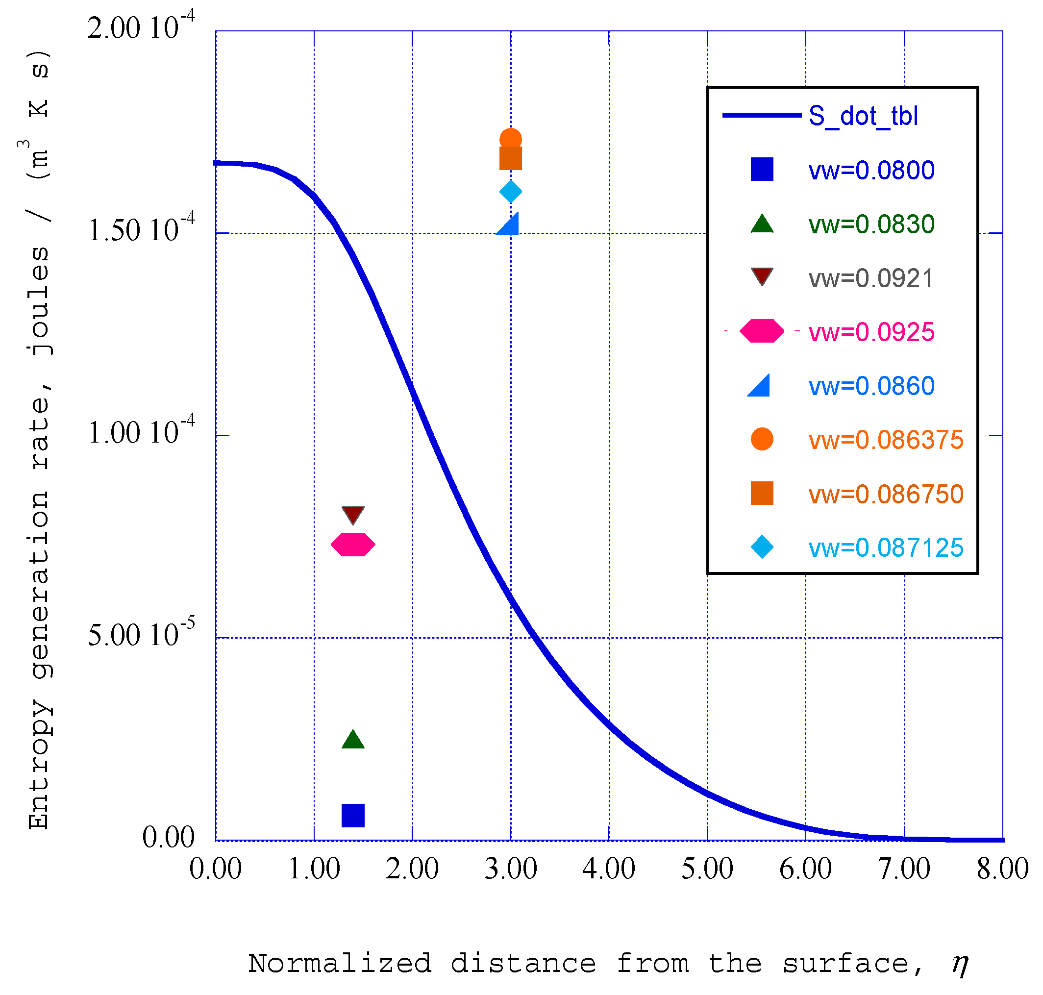
6.3. Entropy Generation Rates for a Turbulent Boundary Layer

For a comparison of these values for the entropy generation rates, the entropy generation rates within a turbulent boundary layer are computed for each given stream wise location. Moore and Moore [24] give the entropy generation rate near the wall in a turbulent boundary layer as:
S t b l = τ w ρ T e ( u y ) w .
Introducing the skin friction coefficient as:
C f = τ w ρ u e 2 2
and applying the Falkner–Skan transformation (Equation (8)) to the velocity gradient, we may write:
S t b l = ρ ( 1 2 u e 2 T ) ( C f ) ( u e x ) ( Re x ) 1 2 ( f ) .
The often-quoted expression for the skin friction coefficient for a turbulent boundary layer on a flat plate may be written as [25]:
C f = 0.0592 ( Re x ) 1 / 5
Substituting this expression for the skin friction coefficient into Equation (43) yields:
S t b l = ρ ( 1 2 u e 2 T e ) ( u e x ) ( 0.0592 ( Re x ) 0.30 ) ( f ) .
This expression is used to compute the entropy generation rates across a hypothetical turbulent boundary layer as a function of the normalized distance η along the horizontal surface of the corner flow configuration. The computation of the turbulent boundary layer begins at the initial station x = 0.02 with transition enforced at this location. Hence, the turbulent boundary layer for our calculations at the stream wise location x = 0.140 is much smaller than for a naturally occurring transition further along the x-direction. The distribution of the entropy generation rates across a flat plate turbulent boundary layer is shown in Figure 16.
The contrast in the fundamental meaning of entropy generation rates between the two sets of data shown in Figure 16 should be clarified. The entropy generation rates computed for the turbulent boundary layer use a well-established empirical relation for the turbulent skin friction coefficient (Equation (44)) and an empirical eddy viscosity expression for the computation of the mean turbulent velocity profile across the boundary layer. These types of results are useful to the designer of thermal power equipment for the estimation of the loss in stagnation pressure due to turbulent irreversible processes within the system.
On the other hand, the computation of the entropy generation rates for the ordered structures proceeds from the identification of time-dependent instabilities within the laminar boundary layer due to nonlinear interactions with an imposed crosswind velocity, through to the evaluation of the dissipation of energy within non-equilibrium ordered structures. With the availability of an appropriate turbulent boundary layer velocity profile, the enhanced skin friction coefficient produced by these ordered structures may then be obtained from the resulting entropy generation rate values. This approach thus introduces basic physical processes into the evaluation of time-dependent non-equilibrium entropy generation processes occurring in this three-dimensional laminar flow environment.

7. Discussion

It has previously been found that a crosswind velocity in a corner boundary layer flow could trigger instabilities in the three-dimensional laminar boundary layer along the horizontal surface [1]. This flow into the boundary layer provides the development of an additional boundary layer profile in the zy plane along the horizontal surface, thus providing a three-dimensional orthogonal boundary layer environment.
Application of coupled, nonlinear modified Lorenz equations in the spectral plane of the flow environment indicates the generation of non-equilibrium spiral structures in the three-dimensional environment. Fluctuating spectral velocity components are found within the three spectral velocity component time-series solutions for these equations. Statistical processing of the solutions indicates the presence of ordered structures embedded within the fluctuating time-series environment. The transition of these ordered structures into equilibrium thermodynamic states yields the entropy generation rates for the overall process.
For the results reported here, the effects of four sidewall injection velocity values are evaluated, we = 0.0800, 0.0830, 0.0921, 0.925, at seven stream wise stations along the x-axis. Each value of crosswind velocity is applied uniformly through the sidewall along the edge of the stream wise boundary layer. The synchronization properties of the modified Lorenz equations are applied from the second to the seventh x-direction stations. Computational results for the initial x-direction station and for the subsequent synchronized stations indicate significant non-equilibrium ordered structure generation at each station at the normalized vertical distance of η = 1.40 in the laminar boundary layer. The intensity of the power spectral densities within these non-equilibrium structures varies from station to station, indicating the triggering of significantly enhanced structures for several stations. It should also be noted that not all of the spectral velocity component time series solutions exhibit fluctuating content. Only the contributions from fluctuating time series solutions from the synchronized stream wise stations are included in the computation of the respective rates of entropy generation.
For example, only the fluctuating spectral velocity components for the two lowest injection velocities contribute to the entropy generation at the second downstream station. At the second stream wise station, x = 0.100, only fluctuations from the lowest injection velocity and the highest injection velocity contribute to the entropy generation, yielding a significantly lower rate of entropy generation.
At the third stream wise station, x = 0.120, the four crosswind velocities indicate high rates of entropy production. The following station, x = 0.140, indicates a significant decrease in entropy generation rates. However, at this station, the power spectral density distribution indicates sharper spectral peaks. We have presented in this article the sequence of the statistical analysis yielding the entropy generation rates for the ordered structures predicted at the stream wise station x = 0.140 at the normalized boundary layer distance of η = 1.40.
To gain a perspective on the magnitude of the predicted rates of entropy generation through the transition of ordered structures, a comparison is made with the rates of entropy generation in a flat plate turbulent boundary layer for the same given flow conditions. The distribution of the entropy generation rates across a turbulent boundary layer at the distance of x = 0.140 is computed for a turbulent boundary layer initiated at x = 0.02 from the leading edge of the horizontal surface. The entropy generation rates through the ordered structures at normalized vertical distances of η = 1.40 and η = 3.0 are then compared with the turbulent boundary layer distribution. At the normalized vertical distance of η = 1.40, the entropy generation rates through the ordered structures are of the same magnitude as the values generated in the turbulent boundary layer. However, at the vertical distance of η = 3.00, the entropy generation rates for the ordered structures considerably exceed those predicted for the turbulent boundary layer. Thus, the influence of the crosswind velocity on the horizontal laminar boundary layer is to initiate instabilities within the laminar boundary layer and to considerably enhance the resulting skin friction coefficient and resulting heat transfer to the horizontal surface [26].
Although the results presented in this article are obtained for the flow configuration of corner flows with sidewall mass injection, the computational procedure is quite generic in its application to general dynamic flow environments. For example, consider the first of three components in the formation of turbulent spots in the transition of laminar to turbulent flows [27]. Initially, a stream wise counter-rotating vortex is formed from a point-wise initiating obstacle. A stream wise laminar boundary layer is initiated on the right side of this vortex, along the floor of the cavity. The counter-rotating vortex produces a crosswind surface boundary layer orthogonal to the stream wise boundary layer [28]. The computational procedure used in the present study appears to be directly applicable to this dynamic flow configuration. The remaining components in the dynamic processes of the transition of laminar to turbulent flows should also be amenable to analysis with the present computational procedure.
However, there are several significant issues concerning the computational procedure discussed in this article. First, the range of kinematic viscosity values for which instabilities have been observed in three-dimensional boundary layer configurations is very narrow [1]. The range of kinematic viscosities that may yield instabilities should be explored to delineate the applicability of the procedure.
Second, there has been no validation of the computational procedure by independent computational results. Inclusion of the time-dependent modified Lorenz equations in the computational procedure should yield additional insight into the process of the transition of laminar to turbulent flow. An independent computational validation would be welcome.
A third issue is that experimental verification of the predicted results is sparse. Results presented in Boiko et al. [29] (pp.120–121) indicate that small amplitude vortices of approximately ten percent of the free-stream velocity in a flat plate boundary layer have been observed. In our calculations, the amplitude of each of the injection crosswind velocities is less than ten percent of the free-stream velocity. In an important experimental measurement, Boiko et al. [29] (pp.115–118) reported the observation of turbulent spots at two vertical locations within a laminar boundary layer, similar to our prediction of the generation of two regions of non-equilibrium ordered structures within the three-dimensional laminar boundary layer in a corner flow with sidewall mass injection. The vertical locations within the boundary layer of the turbulent spots reported in [29] correspond to the vertical locations of the ordered structures reported in this study. This is an important experimental consistency for the results obtained through our computational procedure.

8. Conclusions

An innovative computational procedure for the three-dimensional laminar boundary layer in a corner flow with sidewall mass injection indicates the generation of two regions of non-equilibrium ordered structures within the horizontal laminar boundary layer configuration. The entropy generation rates through the dissipation of these ordered structures are compared. The vertical locations of these ordered structures in the laminar boundary layer are compared with reported experimental observations. Detailed results for the entropy generation rates generated through the dissipation of the ordered structures near the wall are reported. Comparison of the entropy generation rates through the ordered structures with a simulated turbulent boundary layer indicates that the ordered structures near the wall are of similar magnitude, but the dissipation rates for the structures further out are quite strong. These results indicate that transpiration cooling from sidewall injection into a laminar boundary layer may actually increase the heat transfer to the horizontal surface through the generation of these ordered structures. The inclusion of time-dependent non-equilibrium equations into a reservoir of steady laminar boundary layer profiles may provide additional insight into the transition of laminar to turbulent flow.

Acknowledgments

The author would like to thank the editor and referees for their timely and helpful suggestions. Incorporation of these suggestions has significantly strengthened the presentation.

Conflicts of Interest

The author declares no conflict of interest.

Nomenclature

ai
Fluctuating i-th component of velocity wave vector
b
Coefficient in Equation (14)
b
Fluctuating Fourier component of the static pressure
b1
Coefficient in modified Lorenz equations defined by Equation (35)
Cf
Skin-friction coefficient
F
Time-dependent feedback factor
j
Mode number empirical eigenvalue
J
Net source of kinetic energy dissipation rate, Equation (39)
k
Time-dependent wave number magnitude
k
Dimensional constant, Equation (27)
ki
Fluctuating i-th wave number of Fourier expansion
K
Adjustable weighting factor
m
Pressure gradient parameter, Equation (11)
p
Local static pressure
qj
Empirical entropic index for the empirical entropy of mode, j
r1
Coefficient in modified Lorenz equations defined by Equation (33)
s
Entropy per unit mass
s1
Coefficient in modified Lorenz equations defined by Equation (34)
Sempj
Empirical entropy for empirical mode, j
S g e n
Entropy generation rate through kinetic energy dissipation
S t b l
Entropy generation rate in a turbulent boundary layer
t
Time
u
Mean stream wise velocity in the x-direction in Equation (4)
u’
Fluctuating stream wise velocity in Equation (4)
ue
Stream wise velocity at the outer edge of the x-y plane boundary layer
ui
The i-th component of the fluctuating velocity
Ui
Mean velocity in the i-th direction in the modified Lorenz equations
v
Mean normal velocity in Equation (4)
v’
Fluctuating normal velocity in Equation (4)
we
Span wise velocity at the outer edge of the z-y plane boundary layer
x
Stream wise distance
xi
i-th direction
xj
j-th direction
y
Normal distance
z
Span wise distance

Greek Letters

δ
Boundary layer thickness
δlm
Kronecker delta
εm
Eddy viscosity
ε m +
Normalized eddy viscosity
ζj
Intermittency exponent for the j-th mode in Equation (38)
η
Transformed normal distance parameter
λj
Eigenvalue for the empirical mode, j
μ
Mechanical potential in Equation (39)
ν
Kinematic viscosity of the gas mixture
ξj
Kinetic energy dissipation rate in the j-th empirical mode
ρ
Density
σy
Coefficient in modified Lorenz equations defined by Equation (31)
σx
Coefficient in modified Lorenz equations defined by Equation (32)
τw
Wall shear stress

Subscripts 

E
Outer edge of the laminar boundary layer
i, j, l, m
Tensor indices
x
Component in the x-direction
y
Component in the y-direction
z
Component in the z-direction

References

  1. Isaacson, L.K. Entropy Generation through Non-equilibrium Spiral Structures in Corner Flows with Sidewall Surface Mass Injection. Entropy 2016, 18, 47. [Google Scholar] [CrossRef]
  2. Cebeci, T.; Bradshaw, P. Momentum Transfer in Boundary Layers; Hemisphere: Washington, DC, USA, 1977; pp. 319–321. [Google Scholar]
  3. Cebeci, T.; Cousteix, J. Modeling and Computation of Boundary-Layer Flows; Horizons: Long Beach, CA, USA, 2005. [Google Scholar]
  4. Hansen, A.G. Similarity Analyses of Boundary Value Problems in Engineering; Prentice-Hall: Englewood Cliffs, NJ, USA, 1964; pp. 86–92. [Google Scholar]
  5. Townsend, A.A. The Structure of Turbulent Shear Flow, 2nd ed.; Cambridge University Press: Cambridge, UK, 1976. [Google Scholar]
  6. Hellberg, C.S.; Orszag, S.A. Chaotic behavior of interacting elliptical instability modes. Phys. Fluids 1988, 31, 6–8. [Google Scholar] [CrossRef]
  7. Sparrow, C. The Lorenz Equations: Bifurcations, Chaos, and Strange Attractors; Springer: New York, NY, USA, 1982. [Google Scholar]
  8. Attard, P. Non-Equilibrium Thermodynamics and Statistical Mechanics: Foundation and Applications; Oxford University Press: Oxford, UK, 2012. [Google Scholar]
  9. Chen, C.H. Digital Waveform Processing and Recognition; CRC Press: Boca Raton, FL, USA, 1982; pp. 131–158. [Google Scholar]
  10. Press, W.H.; Teukolsky, S.A.; Vetterling, W.T.; Flannery, B.P. Numerical Recipes in C: The Art of Scientific Computing, 2nd ed.; Cambridge University Press: Cambridge, UK, 1992. [Google Scholar]
  11. Rissanen, J. Information and Complexity in Statistical Modeling; Springer: New York, NY, USA, 2007. [Google Scholar]
  12. Tsallis, C. Introduction to Nonextensive Statistical Mechanics; Springer: New York, NY, USA, 2009; pp. 37–43. [Google Scholar]
  13. Arimitsu, T.; Arimitsu, N. Analysis of fully developed turbulence in terms of Tsallis statistics. Phys. Rev. E 2000, 61, 3237–3240. [Google Scholar] [CrossRef] [Green Version]
  14. Isaacson, L.K. Transitional Intermittency Exponents through Non-equilibrium Boundary-Layer Structures and Empirical Entropic Indices. Entropy 2014, 16, 2729–2755. [Google Scholar] [CrossRef]
  15. Mathieu, J.; Scott, J. An Introduction to Turbulent Flow; Cambridge University Press: Cambridge, UK, 2000; pp. 251–261. [Google Scholar]
  16. Manneville, P. Non-equilibrium Structures and Weak Turbulence; Academic Press: San Diego, CA, USA, 1990. [Google Scholar]
  17. Pecora, L.M.; Carroll, T.L. Synchronization in chaotic systems. In Controlling Chaos: Theoretical and Practical Methods in Nonlinear Dynamics; Kapitaniak, T., Ed.; Academic Press: San Diego, CA, USA, 1996; pp. 142–145. [Google Scholar]
  18. Pérez, G.; Cerdeiral, H.A. Extracting messages masked by chaos. In Controlling Chaos: Theoretical and Practical Methods in Nonlinear Dynamics; Kapitaniak, T., Ed.; Academic Press: San Diego, CA, USA, 1996; pp. 157–160. [Google Scholar]
  19. Cuomo, K.M.; Oppenheim, A.V. Circuit implementation of synchronized chaos with applications to communications. In Controlling Chaos: Theoretical and Practical Methods in Nonlinear Dynamics; Kapitaniak, T., Ed.; Academic Press: San Diego, CA, USA, 1996; pp. 153–156. [Google Scholar]
  20. Holmes, P.; Lumley, J.L.; Berkooz, G.; Rowley, C.W. Turbulence, Coherent Structures, Dynamical Systems and Symmetry, 2nd ed.; Cambridge University Press: Cambridge, UK, 2012. [Google Scholar]
  21. De Groot, S.R.; Mazur, P. Non-Equilibrium Thermodynamics; North-Holland: Amsterdam, Holland, 1962. [Google Scholar]
  22. Glansdorff, P.; Prigogine, I. Thermodynamic Theory of Structure, Stability and Fluctuations; Wiley: London, UK, 1971. [Google Scholar]
  23. Mariz, A.M. On the irreversible nature of the Tsallis and Renyi entropies. Phys. Lett. A 1992, 165, 409–411. [Google Scholar] [CrossRef]
  24. Moore, J.; Moore, J.G. Entropy Production Rates from Viscous Flow Calculations: Part I—A Turbulent Boundary Layer Flow. In Proceedings of the 28th ASME International Gas Turbine Conference and Exhibit, Phoenix, AZ, USA, 27–31 March 1983.
  25. White, F.M. Viscous Fluid Flow; McGraw-Hill: New York, NY, USA, 1974. [Google Scholar]
  26. Bayley, F.J.; Turner, A.B. The Transpiration-Cooled Gas Turbine. J. Eng. Power 1970, 92, 351–358. [Google Scholar] [CrossRef]
  27. Cantwell, B.J. Organized Motion in Turbulent Flow. Ann. Rev. Fluid Mech. 1981, 13, 457–515. [Google Scholar] [CrossRef]
  28. Ersoy, S.; Walker, J.D.A. Viscous flow induced by counter-rotating vortices. Phys. Fluids 1985, 28, 2687–2698. [Google Scholar] [CrossRef]
  29. Boiko, A.V.; Grek, G.R.; Dovgal, A.V.; Kozlov, V.V. The Origin of Turbulence in Near-Wall Flows; Springer: Berlin/Heidelberg, Germany, 2010. [Google Scholar]
Figure 1. Schematic of the corner flow boundary layer configuration is shown [1].
Entropy 18 00279 g001
Figure 2. Shown is a three-dimensional deterministic trajectory of the spectral velocity components, ax4, ay4, and az4, at x = 0.140 for η = 1.40 and we = 0.0800.
Entropy 18 00279 g002
Figure 3. The phase diagram of the span wise and normal spectral velocity components, az4ay4, is shown for x = 0.140, η = 1.40 and we = 0.0800.
Entropy 18 00279 g003
Figure 4. A three-dimensional representation of the deterministic trajectories of the spectral velocity components, ax4, ay4, and az4, is shown for x = 0.140, η = 1.40 and we = 0.0925.
Entropy 18 00279 g004
Figure 5. The phase diagram of the span wise and normal spectral velocity components, az4ay4, is shown for x = 0.140, η = 1.40 and we = 0.0925.
Entropy 18 00279 g005
Figure 6. The power spectral density for the normal spectral velocity component is shown for x = 0.140, η = 1.40 and we = 0.0800.
Entropy 18 00279 g006
Figure 7. The power spectral density for the span wise spectral velocity component is shown for x = 0.140, η = 1.40 and we = 0.0800.
Entropy 18 00279 g007
Figure 8. The power spectral density for the normal spectral velocity component is shown for x = 0.140, η = 1.40 and we = 0.0925.
Entropy 18 00279 g008
Figure 9. The power spectral density for the span wise spectral velocity component is shown for x = 0.140, η = 1.40 and we = 0.0925.
Entropy 18 00279 g009
Figure 10. The empirical entropic index for the normal spectral velocity component is shown as a function of the empirical mode, j, for x = 0.140, η = 1.40 and we = 0.0800.
Entropy 18 00279 g010
Figure 11. The empirical entropic index for the normal spectral velocity component is shown as a function of the empirical mode, j, for x = 0.140, η = 1.40 and we = 0.0925.
Entropy 18 00279 g011
Figure 12. The empirical intermittency exponent for the normal spectral velocity component is shown as a function of the empirical mode, j, for x = 0.140, η = 1.40 and we = 0.0800.
Entropy 18 00279 g012
Figure 13. The empirical intermittency exponent for the normal spectral velocity component is shown as a function of the empirical mode, j, for x = 0.140, η = 1.40 and we = 0.0925.
Entropy 18 00279 g013
Figure 14. The entropy generation rates for the non-equilibrium ordered structures at a normalized vertical station η = 1.40 are shown as a function of the x-direction stations for several applied crosswind velocities.
Entropy 18 00279 g014
Figure 15. The entropy generation rates for the non-equilibrium ordered structures at a normalized vertical station η =3.00 are shown as a function of the x-direction stations for several applied crosswind velocities [1].
Entropy 18 00279 g015
Figure 16. The entropy generation rates for various crosswind velocities are shown at normalized distances of η = 1.40 and η = 3.00 at a distance of x = 0.140. Also shown is the distribution of the entropy generation rate at a distance of x = 0.140 for a turbulent boundary layer initiated at x = 0.02 on the horizontal surface.
Entropy 18 00279 g016

