Article

An Entropy-Based Kernel Learning Scheme toward Efficient Data Prediction in Cloud-Assisted Network Environments

1
School of Computer and Communication Engineering, University of Science and Technology Beijing (USTB), Beijing 100083, China
2
Beijing Key Laboratory of Knowledge Engineering for Materials Science, Beijing 100083, China
3
Development and Research Center, China Geological Survey, Beijing 100037, China
4
Key Laboratory of Geological Information Technology, Ministry of Land and Resources, Beijing 100037, China
*
Authors to whom correspondence should be addressed.
Entropy 2016, 18(7), 274; https://doi.org/10.3390/e18070274
Submission received: 13 May 2016 / Revised: 15 July 2016 / Accepted: 18 July 2016 / Published: 22 July 2016
(This article belongs to the Special Issue Information Theoretic Learning)

Abstract

:
With the recent emergence of wireless sensor networks (WSNs) in the cloud computing environment, it is now possible to monitor and gather physical information via lots of sensor nodes to meet the requirements of cloud services. Generally, those sensor nodes collect data and send data to sink node where end-users can query all the information and achieve cloud applications. Currently, one of the main disadvantages in the sensor nodes is that they are with limited physical performance relating to less memory for storage and less source of power. Therefore, in order to avoid such limitation, it is necessary to develop an efficient data prediction method in WSN. To serve this purpose, by reducing the redundant data transmission between sensor nodes and sink node while maintaining the required acceptable errors, this article proposes an entropy-based learning scheme for data prediction through the use of kernel least mean square (KLMS) algorithm. The proposed scheme called E-KLMS develops a mechanism to maintain the predicted data synchronous at both sides. Specifically, the kernel-based method is able to adjust the coefficients adaptively in accordance with every input, which will achieve a better performance with smaller prediction errors, while employing information entropy to remove these data which may cause relatively large errors. E-KLMS can effectively solve the tradeoff problem between prediction accuracy and computational efforts while greatly simplifying the training structure compared with some other data prediction approaches. What’s more, the kernel-based method and entropy technique could ensure the prediction effect by both improving the accuracy and reducing errors. Experiments with some real data sets have been carried out to validate the efficiency and effectiveness of E-KLMS learning scheme, and the experiment results show advantages of the our method in prediction accuracy and computational time.

Graphical Abstract

1. Introduction

A wireless sensor network (WSN) should consist of many sensor nodes in a certain area, and it deals with issues of collecting, processing and transmitting monitored data [1,2]. With the collected data, a WSN is able to detect and evaluate the events occurred just in the monitored field accurately. While WSNs are employed to monitor certain information in an environment, some sensor nodes will collect different information in the system, and that information would be sent to the sink node, which will be used by the end-user. WSNs have been successfully applied to many practical tasks, such as monitoring and early warning, resource management, and so on [3]. Most recently, with the ever-increasing cloud computing services, it places greater demands on efficient data resource acquisition, reconfiguration, and management in cloud-assisted mobile computing environment [4,5,6,7]. Consequently, it also provides an effective support to the applications of WSN. In this paradigm, under the cloud computing environment, it is now possible to monitor and gather physical information via WSN, and those collected data from WSN can be returned from the cloud to the end-users in accordance with their requests [8]. For instance, the integration of WSN and mobile cloud computing is attracting growing interest in both academia and industry, where powerful cloud computing technique is developed to implement processing analysis for the data obtained through WSN and share the results with mobile end-users [9].
There is considerable interest in the paradigm of cloud-assisted WSNs as to the computing strategy of improving working performance in WSNs. Particularly, in a WSN, most devices of sensor nodes have limited power energy and it’s hard to recharge these sensor nodes considering the big amount of those devices in some applications [10]. Furthermore, because the sensed data in a continuous time period are probably closely related to their adjacent data, redundant transmissions between different nodes would accordingly consume much energy [11]. Hence, some data prediction schemes have been proposed to reduce transmissions in a WSN. These schemes make the best of prediction algorithms to lessen redundant transmissions and improve fault tolerance while serving the purpose of reducing energy consumption and hence extending the network life cycle [12,13].
For instance, some computational models and algorithms, including replicated dynamic probabilistic model, auto-regressive model, and cluster-based data fusion scheme, were presented to decrease communication effort [14,15,16]. In addition, some popular machine learning approaches, i.e., least squares support vector machine (LSSVM) and extreme learning machine (ELM), were also used to achieve data prediction in a WSN [11,17]. The detailed analysis for the above methods could be found in Section 2.2. Here, it should be indicated that these methods may have some limitations while achieving ideal prediction performance.
To avoid those limitations, a novel data prediction scheme employing kernel least mean square (KLMS) and information entropy is proposed in this article to decrease unnecessary transfers in WSN. This method is named E-KLMS. KLMS is a typical kernel-based learning algorithm by combining the strategies of memory based iterative learning and error self-correction [18,19,20,21]. For instance, in [21], we applied KLMS to predict missing values in Web QoS data, which is a good application of kernel learning methods. In addition, those random errors could be eliminated by calculating entropy weights [22]. With E-KLMS, the computational complex could be accordingly improved while achieving high-quality solutions. It is worth to note that, different from our previous works [11,23] in which much time are spent in data training because those methods need to construct training set at every sampling point, the samples are only trained once with the proposed method in this article, which will save much time. In consideration of the above reasons, E-KLMS may perform better in data prediction in WSN. In the process of data prediction, two types of nodes employ the same prediction mechanism to maintain data consistency. The end-users define an acceptable threshold. If the derived error is less than a certain threshold, the transmission between different type of nodes is cancelled, meanwhile these nodes would regard the predicted value as the real value at current sampling point. Otherwise, the communication between sink node and sensor node would be normal.
The main contributions in this article are listed as below.
(1)
The sensed data are pretreated using entropy technique before data prediction and fusion. In so doing, it will reduce computational errors while decreasing energy consumption since entropy-based optimization can reduce the size of data set.
(2)
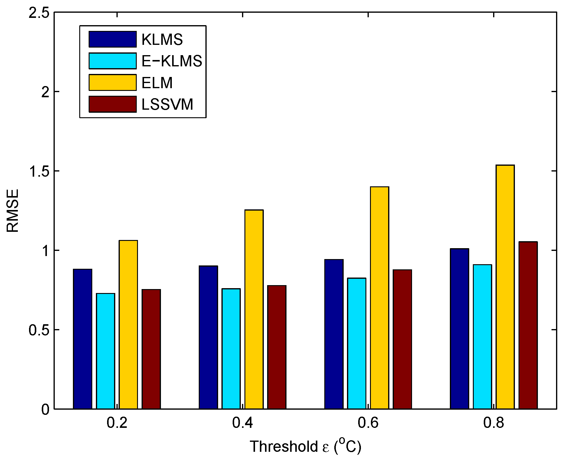
In the flexible working mechanism of keeping the prediction data synchronous in WSN, E-KLMS can achieve better prediction performance regarding the training time and computational accuracy compared with other machine learning methods such as ELM and LSSVM.
This article is organized as below. In Section 2, some related works are analyzed. In Section 3, we present some backgrounds. The entropy-based kernel learning scheme is proposed in Section 4. In Section 5, we provide the experiments, and we summarize the conclusion in Section 6.

2. Related works

2.1. Data Prediction Approaches

Data prediction is now widely used in various fields such as industrial production, economic analysis, and so on. Generally, data prediction approaches could be divided into two major categories, i.e., statistics-based methods and learning-based methods.
The former mainly includes regression model, exponential smoothing model, and autoregressive integrated moving average model (ARIMA). Regression model is an effective tool for data analysis, while revealing the relationship between random variables. However, if there is no correlation between variables, the right results could not be obtained by using it. The exponential smoothing method is widely employed in time series forecasting. But the smooth parameter in single and double exponential smoothing models is unchanged in conventional practices [24]. In statistics and econometrics, ARIMA is widely used under some circumstances with data of non-stationarity, and it could be employed to time series value prediction in the sequence [25]. Then it should define a proper initial different step to avoid the non-stationarity. Nevertheless, the error is increasing with the extension of prediction time.
Considering the limitations of those statistics-based methods, some learning-based methods have been proposed to improve the prediction performance. Usually, they are implemented by using neural network (NN) based and kernel-based machine learning methods. Error back propagation (BP) is a common method of training NN used in conjunction with an optimization method such as gradient descent, but it has low learning efficiency and slow convergence speed [26]. Support vector machine (SVM) is a significant kernel-based machine learning method which is proposed using the structural risk minimization principle rather than the empirical error commonly implemented in the NN, and thus it has better generalization ability and precision compared with traditional NN. However, SVM trains its model periodically and most of its nonlinear identification is offline. Moreover, its computation is very large [27]. Recently, a novel single-hidden layer feedforward network (SLFN) based ELM is proposed to make the predicted value approximate its actual value while achieving a good generalization performance with extremely fast speed [28,29]. But the prediction accuracy of traditional ELM is not satisfying in some cases.
Although basic SVM has its limitations, those kernel-based methods construct an increasing radial basis function network with an increasing memory structure [30]. KLMS is just one of frequently-used and effective kernel-based methods. Moreover, in order to reduce random errors, some techniques are developed to improve the performance of kernel learning methods.

2.2. Prediction Schemes in WSN

Among the available approaches, the replicated dynamic probabilistic model was presented to reduce communications between sensor nodes and sink node in [14]. In this scheme, it is always difficult to effectively mine spatial correlations among sensor nodes unless this model could be maintained while cancelling unnecessary communication between sensors. In [15], the authors proposed a data fusion strategy in WSNs with delay-aware structure, where sensor nodes are divided into many clusters of different sizes and every cluster could contact with the fusion center. However, it is very difficult to achieve ideal effect if the minimum available compression ratio is unknown. In [16], the authors applied auto-regressive modeling technique to WSNs and presented a novel data fusion method. However, the predicted errors are large while dealing with nonlinear data set under certain circumstances. Consequently, a multisensor data fusion method considering quality was presented to overcome a false indication caused by temporary loss of data, signal interference, or invalid data [31]. Meanwhile, to improve the computational efficiency, a method was developed to compute a weighted average of sensor measurements while making the data fusion centre work directly with the compressed data streams [32]. However, the model would become more complicated with the growing of the networks. Recently, many data prediction schemes were accordingly proposed through the use of advanced machine learning algorithms. In [17], a scheme GM-LSSVM in WSN was designed, where the initial prediction is implemented by using grey model (GM) and LSSVM is introduced to reduce the predicted errors. Although the LSSVM-based scheme may achieve a good prediction effect, it is impracticable in some monitoring systems in real time because there is an obstacle of employing LSSVM to predict nonlinear time series online. In [11], the author combined ELM and GM for data fusion. Different from GM-LSSVM, the calculating effort of this scheme is improved greatly due to the fact that the training phase in ELM could be completely implemented with a very fast computational speed. Through this method, the computational time could be reduced greatly. However, its precision would be worse than GM-LSSVM in some applications. Although those schemes improve the performance relating to some metrics, it may be difficult to achieve a good tradeoff between accuracy and computational efforts in WSN [23].

3. Backgrounds

3.1. Problem Statement

In cloud-assisted network environments, the data collected from the WSN will be returned from the cloud to the end-users in accordance with their requests. Figure 1 shows such an example. In an area, some sensor nodes are deployed to gather various information. And those sensory data are transmitted from the WSN to the cloud. Meanwhile, the cloud services are available to the end-users who can conduct some applications through the use of sensory data sent by cloud.
In the cloud-assisted WSN, it is expected that with the use of an effective prediction scheme, the performance of sensor nodes in WSN may be further improved. The prediction process of sensing temperature data in WSN can be described in Figure 2. In this example, the sensor nodes and sink node are supposed to employ the same prediction strategy to keep data synchronous. The sensor node sends the first 2500 data points to the sink node. Then they both conduct training to seek the hidden relationship between inputs and outputs, and then predict the following data points. If the predicted error is less than a certain threshold, the prediction value is considered as the actual value while cancelling the transmission between sink node and sensor node. Otherwise, the sensor node must respond to the sink node by sending its actual sensed data that are described by the red points in Figure 2.

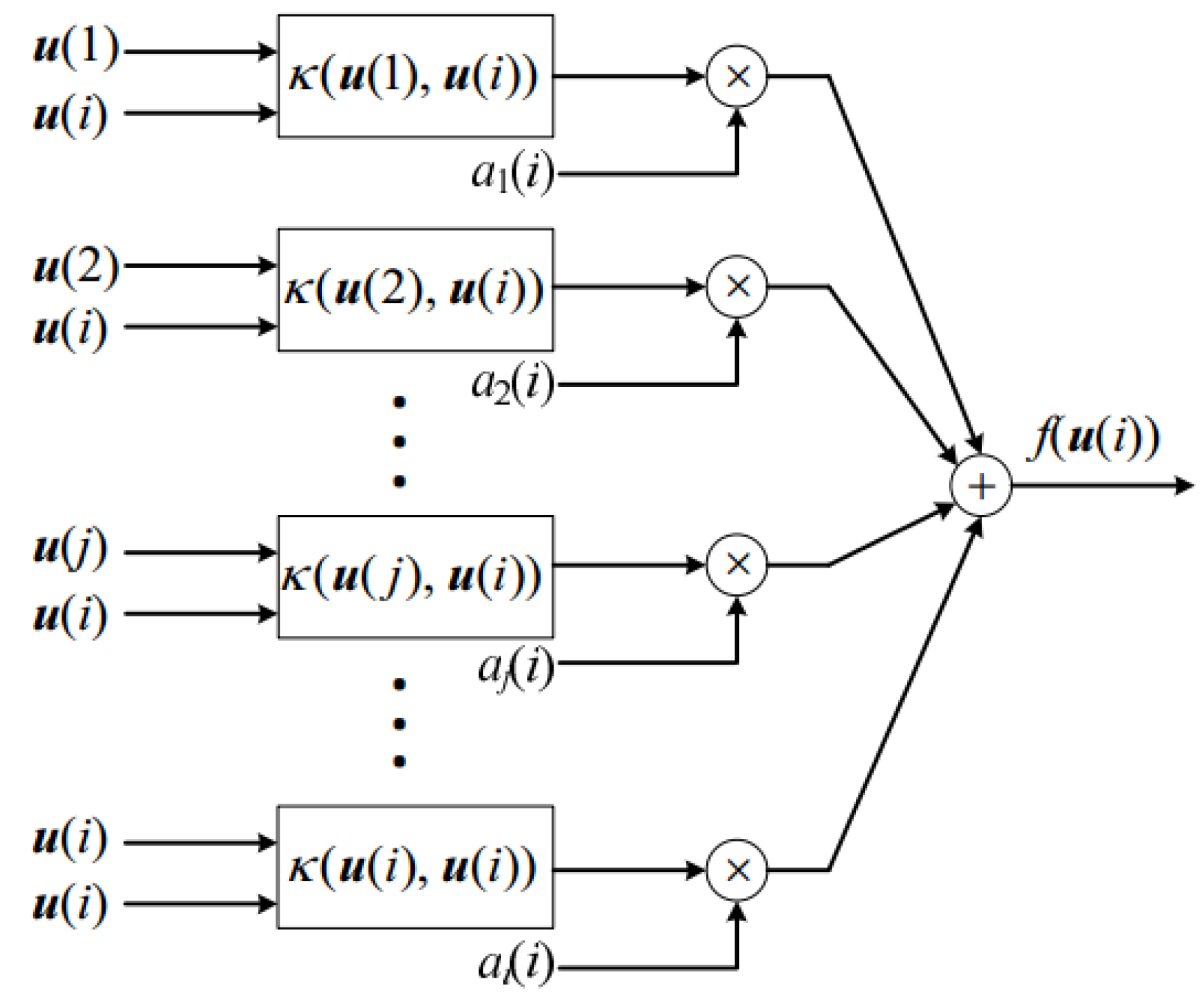
3.2. Kernel Least Mean Square Algorithm

In the past few years, the idea of least mean square (LMS) finds a wide application in the field of engineering computing, but it is not suitable for nonlinear cases. In view of it, KLMS is proposed to deal with nonlinear data [30]. At iteration i, the kernel function is employed to transform the input u ( i ) into a high-dimensional feature space F as ψ ( u ( i ) ) . Applying LMS on the basis of the data sequence { ψ ( u ( i ) ) , γ ( u ( i ) ) } and we could get
ξ ( u ( i ) ) = γ ( u ( i ) ) [ ν ( u ( i 1 ) ) ] T ψ ( u ( i ) )
ν ( u ( i ) ) = ν ( u ( i 1 ) ) + λ ξ ( u ( i ) ) ψ ( u ( i ) )
where ν ( u ( i ) ) indicates the estimation of the weight vector in higher dimensional space, γ ( u ( i ) ) denotes the desired output, and λ denotes the step-size parameter. Generally, we define ν ( u ( 0 ) ) = 0 . By repeating rules Equations (1) and (2) through iterations and we could get
ν ( u ( i ) ) = ν ( u ( i 1 ) ) + λ ξ ( u ( i ) ) ψ ( u ( i ) ) = [ ν ( u ( i 2 ) ) + λ ξ ( u ( i 1 ) ) ψ ( u ( i 1 ) ) ] + λ ξ ( u ( i ) ) ψ ( u ( i ) ) = ν ( u ( i 2 ) ) + λ [ ξ ( u ( i 1 ) ) ψ ( u ( i 1 ) ) + ξ ( u ( i ) ) ψ ( u ( i ) ) ] = ν ( u ( 0 ) ) + λ j = 1 i ξ ( u ( j ) ) ψ ( u ( j ) ) = λ j = 1 i ξ ( u ( j ) ) ψ ( u ( j ) )
Then, the weight estimation is characterized by all the former inputs, and its value depends on the predicted errors and step-size parameter. After that, with the given input u , the output value could be summarized as below
ν ( u ( i ) ) T ψ ( u ) = λ j = 1 i ξ ( u ( j ) ) [ ψ ( u ( j ) ) ] T ψ ( u ) = λ j = 1 i ξ ( u ( j ) ) [ ψ ( u ( j ) ) ] T ψ ( u )
According to the kernel mapping Equation (5), we could obtain the filter outputs on the basis of kernel evaluations
[ ψ ( u ) ] T ψ ( u ) = κ ( u , u )
[ ν ( u ( i ) ) ] T ψ ( u ) = λ j = 1 i ξ ( u ( j ) ) κ ( u ( j ) , u )
where κ denotes a mapping function. And a function with Gaussian kernel could be expressed by
κ ( u , u ) = exp ( a u u 2 )
Here, a is the parameter of kernel.
Consider f i as the mapping relationship between the inputs and outputs at iteration i, thus the computational procedure of KLMS can be summarized as follows
f i 1 ( · ) = λ j = 1 i 1 ξ ( u ( j ) ) κ ( u ( j ) , · )
f i ( · ) = f i 1 ( · ) + λ ξ ( u ( i ) ) κ ( u ( i ) , · )
f i 1 ( u ( i ) ) = λ j = 1 i 1 ξ ( u ( j ) ) κ ( u ( j ) , u ( i ) )
ξ ( u ( i ) ) = γ ( u ( i ) ) f i 1 ( u ( i ) )
KLMS is shown in Algorithm 1 [30] and a diagram is given in Figure 3. Then, a ( i ) represents the coefficient in the i-th iteration, and a ( i ) = a j ( i ) j = 1 i = λ ξ ( u ( j ) ) j = 1 i . Besides, C ( i ) represents the center set. With the new input vector u * in the i-th iteration, we can obtain its corresponding output
f i ( u * ) = λ j = 1 i ξ ( u ( j ) ) κ ( u ( j ) , u * )
Algorithm 1 KLMS Algorithm
select the kernel κ and a proper step parameter λ, i = 1 ;
a 1 ( 1 ) = λ ξ ( u ( 1 ) ) , C ( 1 ) = { u ( 1 ) } , f 1 ( · ) = a 1 ( 1 ) κ ( u ( 1 ) , · ) ;
for { u ( i ) , γ ( u ( i ) ) } do
(1)
calculate output value: f i 1 ( u ( i ) ) = j = 1 i 1 a j ( i 1 ) κ ( u ( j ) , u ( i ) ) ;
(2)
calculate error: ξ ( u ( i ) ) = γ ( u ( i ) ) f i 1 ( u ( i ) ) ;
(3)
update center set: C ( i ) = { C ( i 1 ) , u ( i ) } ;
(4)
calculate coefficients: a i ( i ) = λ ξ ( u ( i ) ) ;
(5)
update: i = i + 1 ;
end for

3.3. Information Entropy

Information entropy could survey the disordered measurement of information. The bigger the information entropy, the less effective information it contains in a system [33]. On the contrary, the smaller the information entropy, the more useful information it contains in the system. Here, the entropy of a variable X is defined as follows
H ( X ) = x X p ( x ) log b p ( x )
where p ( x ) represents the probability of x, and b is assigned a value of 2 or e. Through the use of information entropy rules, the entropy weight method is developed to measure how much information the variable contains. The calculation steps are as follows.
For a data matrix U = [ u i j ] m × n = [ u 1 , u 2 , , u n ] where u j denotes the j-th input vector and u j = [ u 1 j , u 2 j , , u m j ] T ( 1 j n ) , the data is standardized as follows
u i j + = u i j i = 1 m u i j
Then, a new matrix could be obtained by U + = [ u i j + ] m × n .
The information entropy of the j-th input vector u j is
e j = k i = 1 m u i j + ln ( u i j + )
Here, k is a constant which is related to the dimension of input vector m. Suppose that the system is in a complete disorder (i.e., u i j + = 1 m ), the entropy value H = 1 . We have
H = k i = 1 m 1 m ln 1 m = k ln m = 1
So, k = 1 ln m . Then, 0 e j 1 .
For the j-th input vector, the validity coefficient h j is defined by
h j = 1 e j , 0 h j 1
By applying Equation (17), the entropy weight of each input vector can be defined by
w j = h j j = 1 n h j
It can be seen from the above equations, the bigger the entropy weight, the more effective information the input vector contains. In addition, it means that the vector is more important to the whole system. Otherwise, the input vector is less important. Specifically, we use this entropy weight to evaluate and optimize the input data in our kernel learning scheme.

4. E-KLMS Scheme

4.1. Learning and Prediction in the Proposed Scheme

Aiming at addressing the nonlinear property of data set to reduce prediction error and achieve a better prediction performance, we present an entropy-based scheme called E-KLMS with the help of strong generalization ability of kernel learning method. In the proposed scheme, the entropy weights of input vectors are firstly calculated to measure their importance. Then we remove those input vectors whose entropy weights are less than the average value. Meanwhile their corresponding outputs are also removed. By this means, the original data set is optimized. Finally, we train the KLMS learning model with the modified training set to find out the hidden relationships between inputs and outputs. Through the use of the relationships and given inputs, the output values therefore can be predicted.
There are five steps in our proposed method. The specific descriptions are shown as below.
(1)
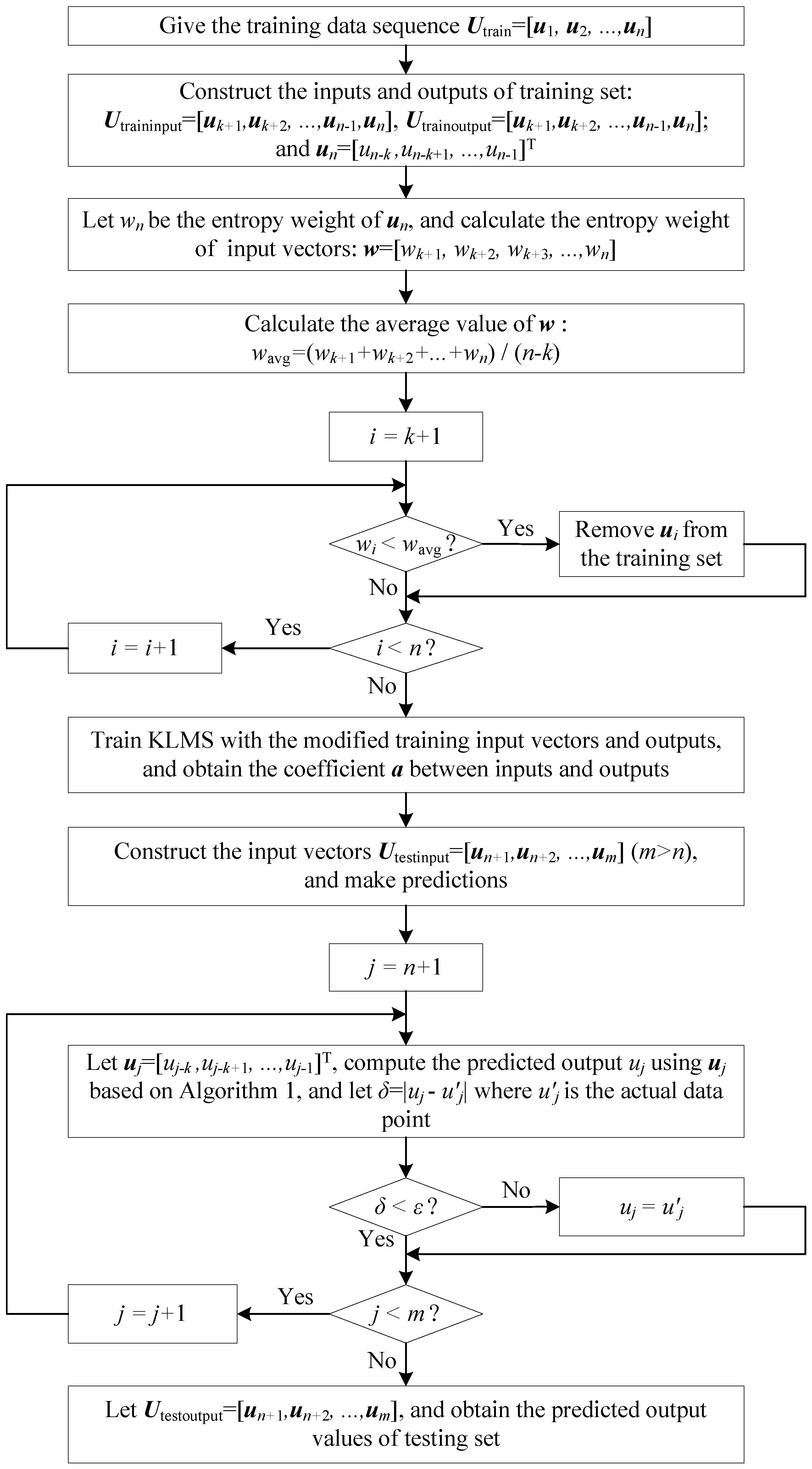
The default predicted error threshold ε will be sent to all working sensor nodes, and all sensor nodes deliver the first n actual values to the sink node which are used as training set data.
(2)
These two kinds of nodes implement prediction according to the same prediction strategy and data set. Here is the sequence: U train = [ u 1 , u 2 , , u n ] where n indicates the size of data points, the inputs and outputs of training set are constructed as follows
U traininput = [ u k + 1 , u k + 2 , , u n 1 , u n ]
U trainoutput = [ u k + 1 , u k + 2 , , u n 1 , u n ]
Here k denotes the dimension of input vectors and u n = [ u n k , u n k + 1 , , u n 1 ] T .
(3)
The entropy weight of each input vectors is calculate on the basis of Equations (14)–(18). Then, we have
w = [ w k + 1 , w k + 2 , w k + 3 , , w n ]
where w n denotes the entropy weight of u n .
(4)
After comparing entropy weights of all input vectors with the average entropy weight, we remove those input vectors whose entropy weights are less than the average value, and their corresponding outputs are deleted from training set at the same time.
(5)
With the modified training set, the KLMS learning model is trained. Then, the coefficient a between inputs and outputs is obtained. And it reveals the hidden relationships between inputs and outputs.
(6)
The testing input vector is constructed through the use of its previous k data points. Next, the prediction is conducted by using Algorithm 1. If the prediction error δ is less than ε, the transmission between these two type of nodes will be cancelled and the prediction value will be considered as the real value. Repeat this step until all the outputs are predicted.
Finally, the details of our approach E-KLMS is shown in Figure 4.

4.2. Analysis of Complexity

We briefly analyze the time complexity of the scheme proposed in this article. Obviously, E-KLMS spends most of the time on entropy calculating and KLMS model training. For every input vector in training set, the calculations would be conducted k times for generating the entropy weight, where k denotes the dimension of input vectors. And the number of input vectors in training set is n. Hence, the computational complexity of entropy calculation is O ( k n ) . Similarly, the learning complexity of KLMS is also O ( k n ) [34,35]. Consequently, it could be concluded that the complexity of E-KLMS is also O ( k n ) .
Moreover, in [34], it was noted that the time complexity of ELM for n samples and k bases models is O ( k n + k 3 ) . When n is much larger than k, the complexity of ELM approximately equals to O ( k n ) . That is to say, if the size of data set is large enough, the time complexities of these methods mentioned above could be considered as the same.

5. Experiments and Discussion

5.1. Experiment Settings

Here, our experiments are concerned with the purpose of verifying the effectiveness of the proposed intelligent data prediction scheme. It should be noted that as shown in Figure 1, we do not provide other experiments for the data transmission and processing in the cloud computing environment since they are implemented in the usual way. We import two real data sets into our experiments. Considering the analysis in Section 1 and Section 2, some traditional schemes have some limitations. The computational speed of LSSVM is not fast enough, and ELM has very fast computational speed but its precision may be unsatisfactory for some practical tasks. Meanwhile, KLMS may perform worse than LSSVM in some situations. Hence, we carry out experiments with some comparisons among our scheme, KLMS, ELM, and LSSVM to validate the computational speed and precision. LSSVM algorithm mentioned here is realized by employing the MATLAB Toolbox [36,37].
The real data sets are obtained from Intel Berkeley lab, and the distribution of sensor nodes is shown in Table 1 [38]. Here, the X and Y coordinates of sensors are in meters relative to the upper right corner of the lab. These sensor nodes obtain different type of data, regarding temperature, humidity, and light. We select one sensor node randomly in the experiments to test the algorithm performance on predicting its humidity and temperature data. It contains 4000 continuous data values, where the first 3000 data points are employed to construct training set and the following 1000 data points will be predicted. As mentioned above, ε denotes the threshold defined by end-users. Therefore, we compare the prediction errors, computational time, and prediction precision with various threshold ε. Moreover, to achieve optional prediction effect, the kernel parameter a and step-size parameter λ are chosen from the range { 2 1 , 2 2 , 2 3 , , 2 20 } , respectively.

5.2. Metrics

In addition to successful prediction rate, two metrics, including the root mean squared error (RMSE) and the mean absolute error (MAE), are selected to test prediction precision in our experiments. Their definitions are summarized as below
RMSE = 1 N j = 1 N | u j u j | 2
MAE = 1 N j = 1 N | u j u j |
where u j is the predicted value and u j is the actual value. Generally, a larger RMSE or MAE indicates a worse effect.
From Equation (19), the squares of predicted errors are firstly calculated, and the average value is accordingly obtained. Then, calculating the square root is conducted. Therefore, this metric works when decreasing the influence of large errors.

5.3. Analysis for the Implementation of Our Work

As we know, WSN in cloud-assisted network environments have become so widespread in many special fields, where data prediction and fusion schemes are rapidly developed. Thus, improving the prediction precision and reducing the energy consumption are becoming increasingly important. Aiming at such issues of improving accuracy, calculation effort, and implementation framework, we propose an efficient data prediction scheme combining KLMS and information entropy. There are some obvious advantages during the implementation of our scheme. Firstly, the synchronization mechanism in this article could greatly improve the fault tolerance of sensor nodes in WSN. Actually, if there is something wrong with sensor node at some time, the sink node is able to predict data values without receiving data from the wrong sensor node, which will be really helpful in cloud computing environment. Secondly, since the sensor nodes have limited power and it is hard to charge the batteries, reducing energy consumption is urgently needed. Data pretreatment with entropy technique will decrease the size of data set and calculation effort. By this means, energy consumption could be immensely reduced. Thirdly, in addition to monitoring system, the proposed scheme could also be employed to other practical applications with information interaction in cloud-assisted network environments.

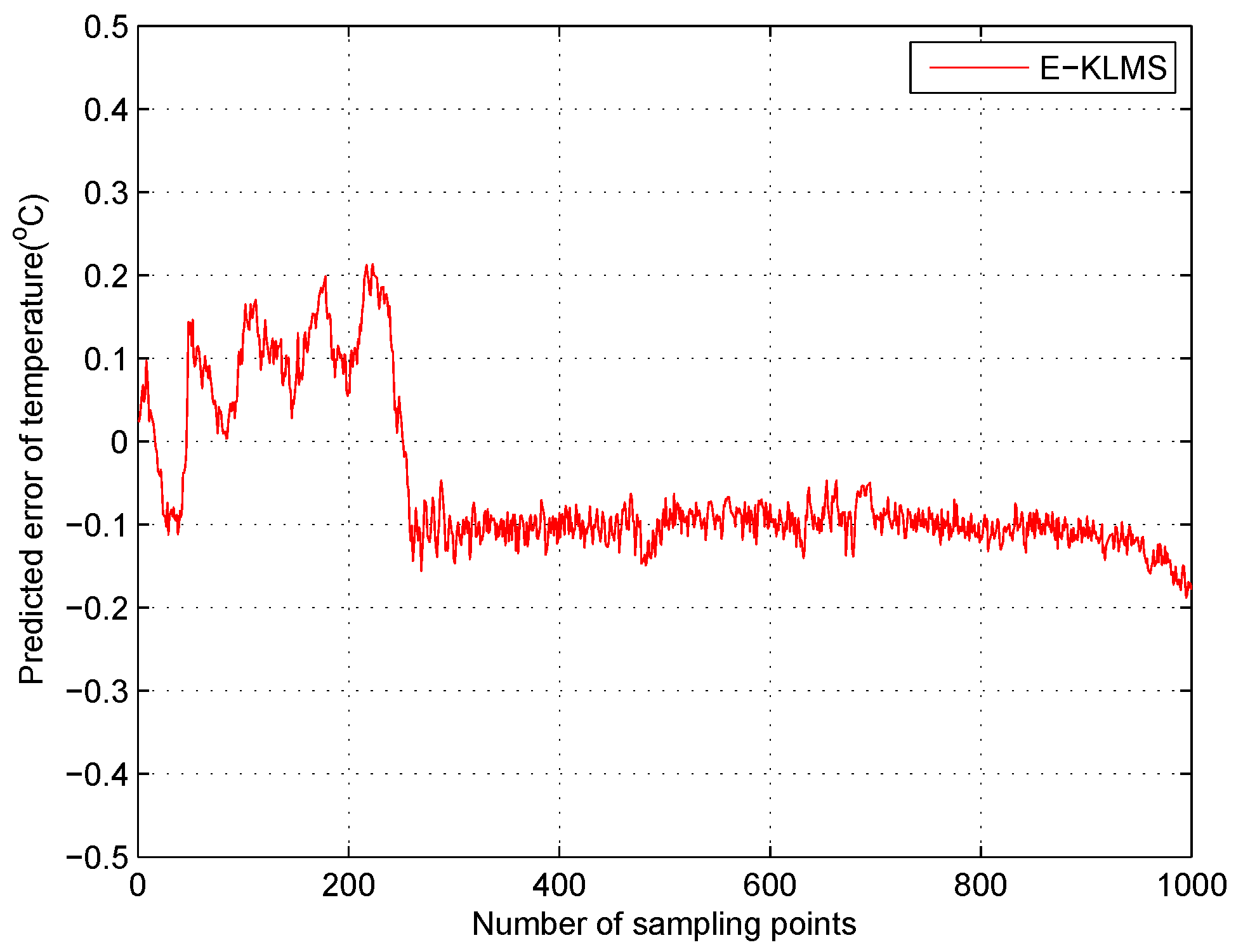
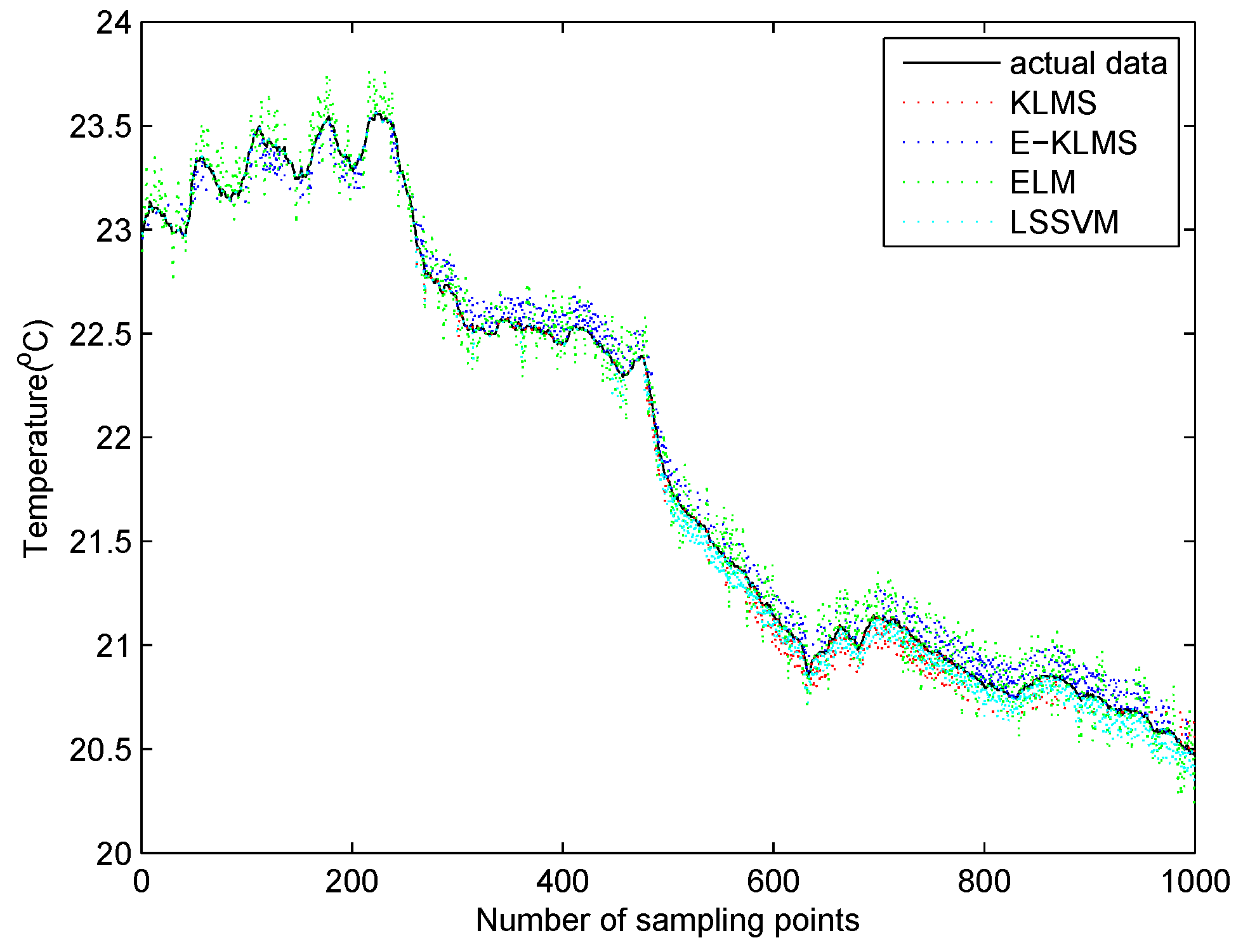
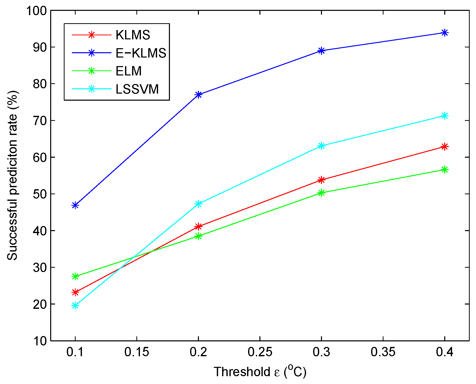
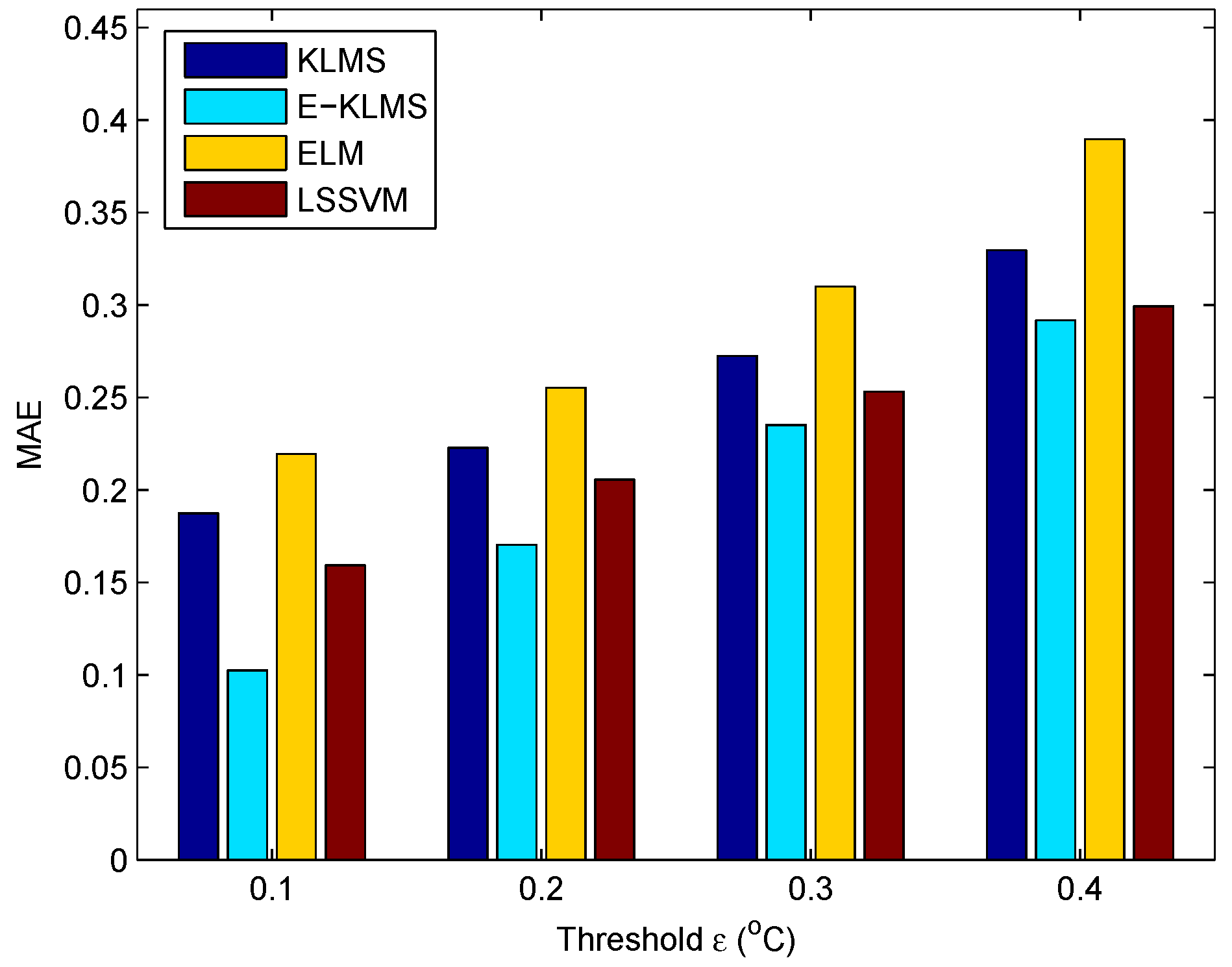
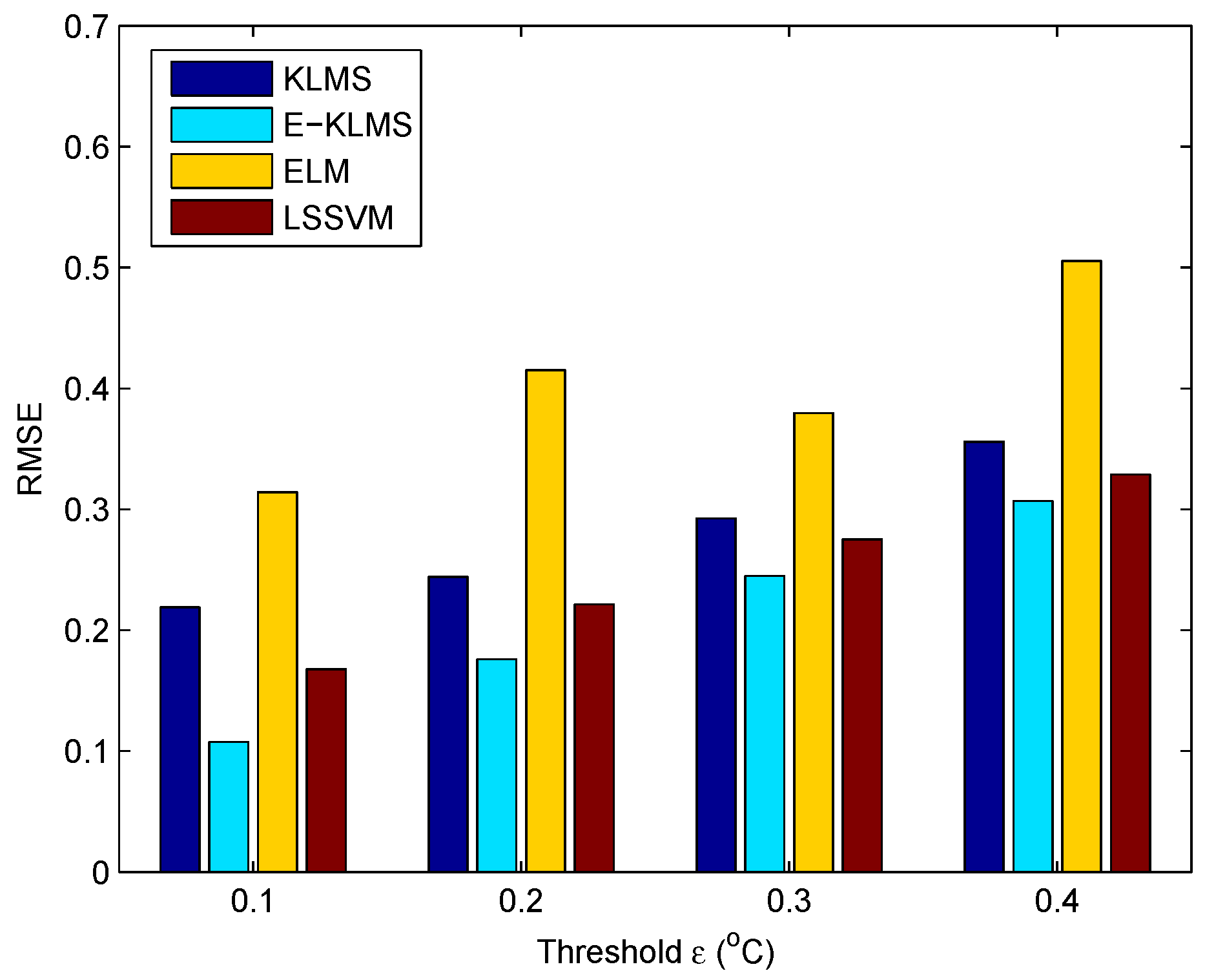
5.4. Test Case in Temperature Data Set

Figure 5 depicts the prediction effect for temperature set when ε = 0.2 . It could be seen that the predicted values of four schemes are consistent with the real values. Figure 6 provides a comparison for the successful predicted rate as ε changes. It is obvious that as the threshold increases, E-KLMS always has the highest successful prediction rate. In other words, compared with other schemes, it will produce less communication overhead in WSN through the use of E-KLMS. Thus, the goal of saving energy and extending lifetime of the whole WSN could be achieved.
Figure 7 and Figure 8 show the MAE and RMSE of these four schemes when the threshold ε changes. A smaller MAE or RMSE indicates a better forecast effect. The figures show that the MAE and RMSE of E-KLMS are minimum. As the threshold ε increases, the performances of LSSVM is very close to E-KLMS. Meanwhile, the comparison between KLMS and E-KLMS demonstrates the superiority of our proposed scheme. Considering the above results, the whole forecast effect of E-KLMS is best.
Particularly, when ε = 0.2 , the prediction errors while using E-KLMS are shown in Figure 9. It could be observed that the errors are restricted within a small scope.

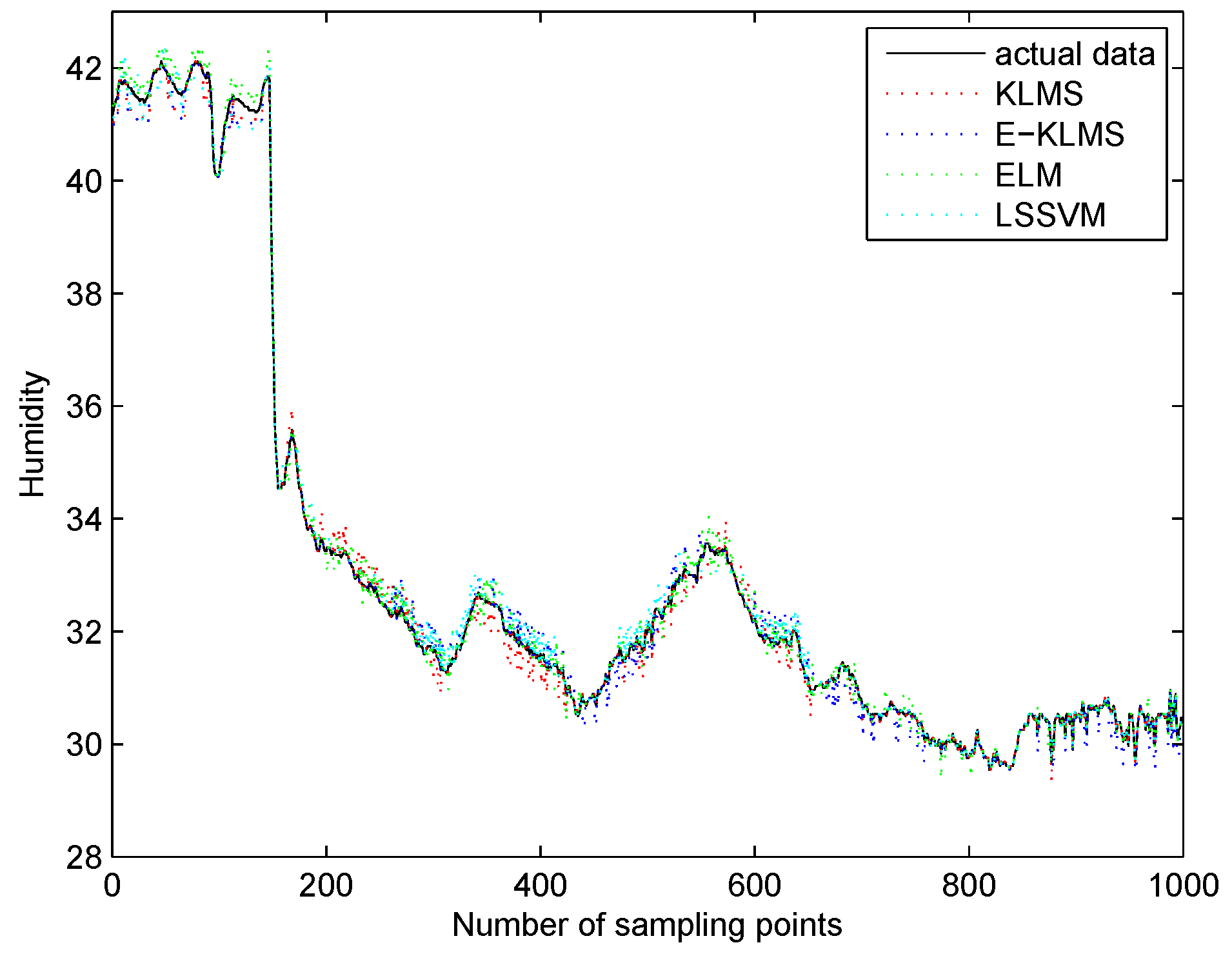
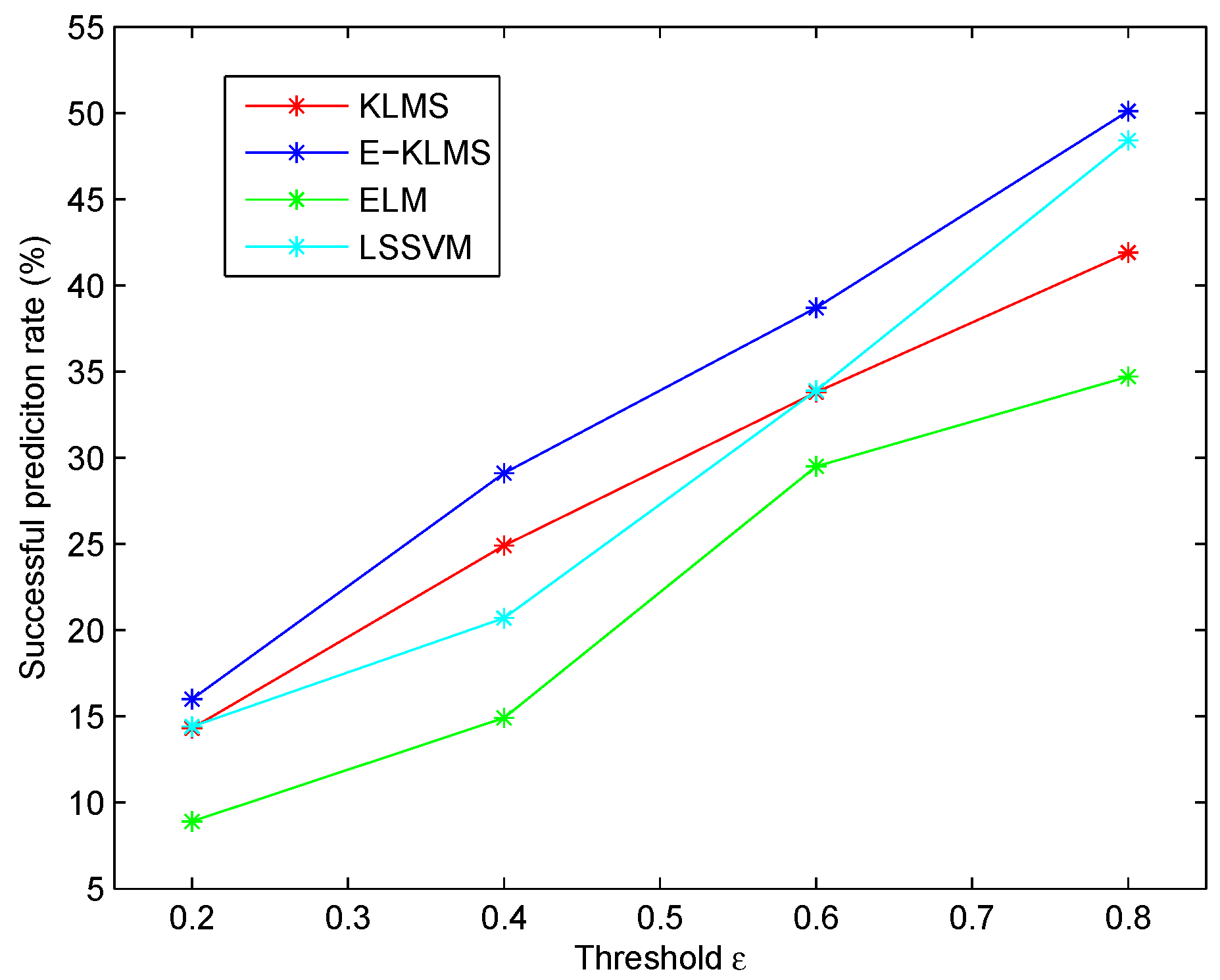
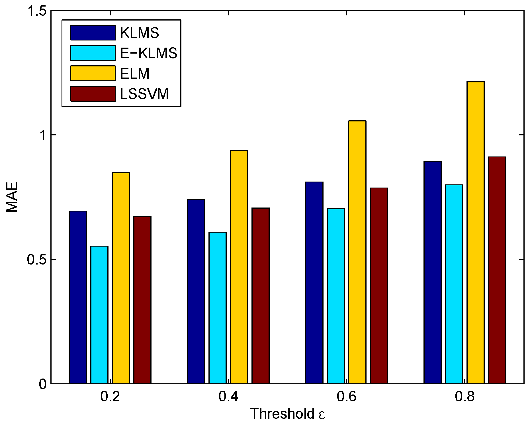
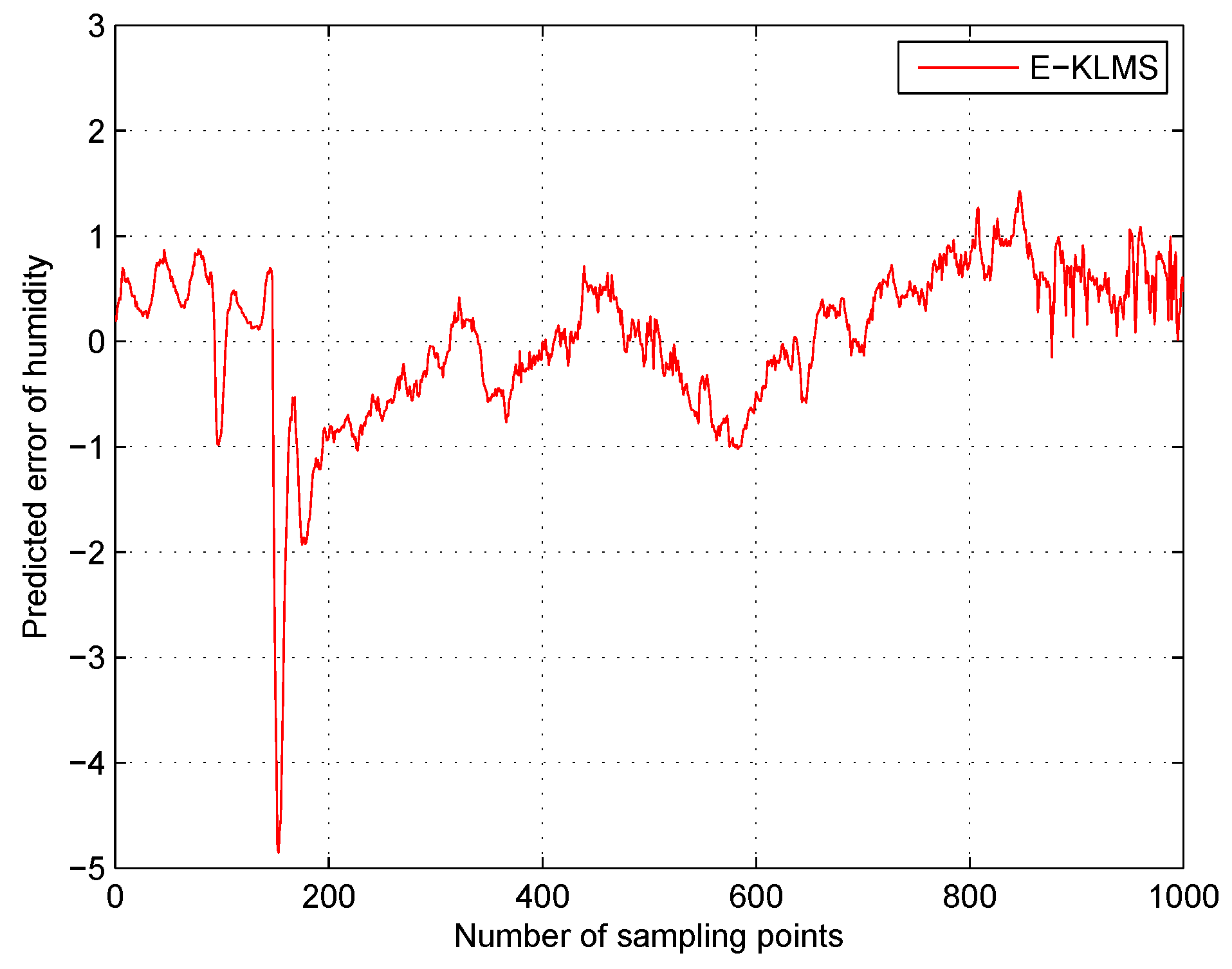
5.5. Test Case in Humidity Data Set

When ε = 0.4 , the real humidity value and the predicted value using four schemes at every data point are demonstrated in Figure 10. It can be observed that the predicted results of these four methods are consistent with the real humidity data.
However, at some sampling points, ELM, LSSVM, and KLMS perform worse with bigger errors than E-KLMS. In the proposed method, the data containing less information which may have a negative impact in prediction process, is removed from training data. Therefore, the prediction effect of E-KLMS is better than other three schemes.
Moreover, Figure 11 shows the successful prediction rate with various threshold ε. The result of LSSVM approximates to that of E-KLMS. ELM has the minimal successful prediction rates and E-KLMS has the maximal ones.
Figure 12 and Figure 13 show the corresponding MAE and RMSE of these four schemes when the threshold ε changes. Similarly, the MAE and RMSE of E-KLMS are minimum. When ε = 0.4 , Figure 14 shows the prediction errors of E-KLMS.
Furthermore, we compare the whole computational effort of these methods in data fusion and prediction process. The results are listed in Table 2. Specifically, we also compare the average computational effort of these four schemes for predicting a single data. The results are listed in Table 3. It is clear that ELM spends least time in calculation and the computational cost of LSSVM is much more than other schemes. Meanwhile, E-KLMS spends less time than KLMS in calculation. Although E-KLMS takes more time in entropy weight computation, its computational complexity will be decreased after optimizing the training set. Generally, calculation effort is closely related to energy consumption. If the sensor node spends less time in calculation, its energy consumption will be accordingly reduced.
Considering the time consumption and prediction precision, our scheme E-KLMS is a better choice in this application field. Even though ELM spends less time in calculation, it is difficult to choose proper design parameters during the implementation process. Then, the prediction accuracy of ELM may be lower than other methods. Meanwhile, LSSVM has preferable prediction effect, but it takes a very long period of time in computation. KLMS learning algorithm just maps the data into high-dimensional feature space, through adjusting itself adaptively to the projection. Hence, with every input vector, KLMS is concerned with the function space. To that end, through a combination of KLMS and entropy weight technique, E-KLMS has its superiority when using the proposed computational paradigm.

6. Conclusions

Generally, in cloud-assisted network environment, the sensed data values in a continuous time period are closely related to their adjacent data, and the storage space and energy of sensor nodes are limited. Hence, the data prediction technique in WSN is so popular with the purpose of decreasing energy consumption, cancelling unnecessary data transmissions, and extending the network life cycle. A data prediction scheme E-KLMS using KLMS and entropy is accordingly developed to deal with the problems analyzed here. The presented scheme employs a forecast technique to maintain the data consistency. During the data prediction process, the entropy weights of training set inputs are firstly calculated. Then, for the inputs and their corresponding outputs whose entropy are less than the average value, we remove them which may cause relatively large errors in prediction. Next, through the use of KLMS, the training operation is conducted to find the hidden relationships between inputs and outputs. On the basis of it, the following data value could be predicted. E-KLMS could effectively solve the tradeoff problem between precision and calculation effort while immensely simplifying the training process. Furthermore, entropy-based kernel learning method ensures the prediction performance through improving the accuracy and reducing errors. It can be seen from the experimental results that our scheme can efficiently decrease redundant transmissions while improving the prediction precision. By this means, the energy of sensor nodes is also saved and the fault tolerance is improved. Meanwhile, the experimental comparisons between E-KLMS and other traditional schemes are implemented. The prediction accuracy of ELM is not satisfying although its computational speed is really fast compared with other schemes. On the contrary, the prediction effect of LSSVM is so good, but it spends too much time on computation. The proposed scheme E-KLMS performs best according to prediction precision, and its calculation speed is also competitive. Furthermore, through the comparison of E-KLMS and KLMS, both the prediction accuracy and computation metrics demonstrate the effectiveness of information entropy used in our scheme. In view of those facts mentioned above, E-KLMS may be a better choice in cloud-assisted network environment for WSN.

Acknowledgments

This research is funded by the National Natural Science Foundation of China under Grants 61174103, 61272357, and 61300074, the National Key Technologies R&D Program of China under Grant 2015BAK38B01, the China Postdoctoral Science Foundation under Grant 2016M590048, and the Fundamental Research Funds for the Central Universities under Grant 06500025.

Author Contributions

In this article, Xiong Luo and Weiping Wang provided the original ideas and were responsible for revising the whole article; Ji Liu and Dandan Zhang designed and performed the experiments; Yueqin Zhu analyzed the data. All authors have read and approved the final manuscript.

Conflicts of Interest

The authors declare no conflict of interest.

References

  1. Yick, J.; Mukherjee, B.; Ghosal, D. Wireless sensor network survey. Comput. Netw. 2008, 52, 2292–2330. [Google Scholar] [CrossRef]
  2. Oliveira, L.M.; Rodrigues, J.J. Wireless sensor networks: A survey on environmental monitoring. J. Commun. 2011, 6, 1796–2021. [Google Scholar] [CrossRef]
  3. Nam, Y.; Rho, S.; Lee, B.G. Intelligent context-aware energy management using the incremental simultaneous method in future wireless sensor networks and computing systems. EURASIP J. Wirel. Commun. Netw. 2013, 2, 146–155. [Google Scholar] [CrossRef]
  4. Baccarelli, E.; Cordeschi, N.; Mei, A.; Panella, M.; Shojafar, M.; Stefa, J. Energy-efficient dynamic traffic offloading and reconfiguration of networked data centers for big data stream mobile computing: Review, challenges, and a case study. IEEE Netw. 2016, 30, 54–61. [Google Scholar] [CrossRef]
  5. Shojafar, M.; Cordeschi, N.; Baccarelli, E. Energy-efficient adaptive resource management for real-time vehicular cloud services. IEEE Trans. Cloud Comput. 2016, PP. [Google Scholar] [CrossRef]
  6. Ryu, S.; Chen, A.; Choi, K. Solving the stochastic multi-class traffic assignment problem with asymmetric interactions, route overlapping, and vehicle restrictions. J. Adv. Transp. 2016, 50, 255–270. [Google Scholar] [CrossRef]
  7. Canali, C.; Lancellotti, R. Detecting similarities in virtual machine behavior for cloud monitoring using smoothed histograms. J. Parallel Distrib. Comput. 2014, 74, 2757–2759. [Google Scholar] [CrossRef] [Green Version]
  8. Yu, C.M.; Chen, C.Y.; Chao, H.C. Verifiable, privacy-assured, and accurate signal collection for cloud-assisted wireless sensor networks. IEEE Commun. Mag. 2015, 53, 48–53. [Google Scholar] [CrossRef]
  9. Zhu, C.; Leung, V.C.M.; Yang, L.T.; Shu, L. Collaborative location-based sleep scheduling for wireless sensor networks integrated with mobile cloud computing. IEEE Trans. Comput. 2015, 64, 1844–1856. [Google Scholar] [CrossRef]
  10. Esch, J. A survey on topology control in wireless sensor networks: Taxonomy, comparative study, and open issues. Proc. IEEE 2013, 101, 2534–2537. [Google Scholar] [CrossRef]
  11. Luo, X.; Chang, X.H. A novel data fusion scheme using grey model and extreme learning machine in wireless sensor networks. Int. J. Control Autom. Syst. 2015, 13, 539–546. [Google Scholar] [CrossRef]
  12. Yang, F.C.; Yang, L.L. Low-complexity noncoherent fusion rules for wireless sensor networks monitoring multiple events. IEEE Trans. Aerosp. Electron. Syst. 2014, 50, 2343–2353. [Google Scholar] [CrossRef]
  13. Nakamura, E.F.; Loureiro, A.A.F.; Frery, A.C. Information fusion for wireless sensor networks: Methods, models, and classifications. ACM Comput. Surv. 2007, 39, 415–416. [Google Scholar] [CrossRef]
  14. Chu, D.; Deshpande, A.; Hellerstein, J.M.; Hong, W. Approximate data collection in sensor networks using probabilistic models. In Proceedings of the 22nd International Conference on Data Engineering, Atlanta, GA, USA, 3–7 April 2006; pp. 48–60.
  15. Cheng, C.T.; Leung, H.; Maupin, P. A delay-aware network structure for wireless sensor networks with in-network data fusion. IEEE Sens. J. 2013, 13, 1622–1631. [Google Scholar] [CrossRef]
  16. Hui, A.; Cui, L. Forecast-based temporal data aggregation in wireless sensor networks. Comput. Eng. Appl. 2007, 43, 121–125. [Google Scholar]
  17. Wang, R.; Tang, J.; Wu, D.; Sun, Q. GM-LSSVM based data aggregation in WSN. Comput. Eng. Des. 2012, 33, 3371–3375. [Google Scholar]
  18. Liu, W.F.; Pokharel, P.P.; Principe, J.C. The kernel least-mean-square algorithm. IEEE Trans. Signal Process. 2008, 56, 543–554. [Google Scholar] [CrossRef]
  19. Chen, B.D.; Zhao, S.L.; Zhu, P.P.; Principe, J.C. Quantized kernel least mean square algorithm. IEEE Trans. Signal Process. 2012, 23, 22–32. [Google Scholar]
  20. Chen, B.D.; Zhao, S.L.; Zhu, P.P.; Principe, J.C. Quantized kernel recursive least squares algorithm. IEEE Trans. Neural Netw. Learn. Sys. 2013, 24, 1484–1491. [Google Scholar] [CrossRef] [PubMed]
  21. Luo, X.; Liu, J.; Zhang, D.D.; Chang, X.H. A large-scale web QoS prediction scheme for the industrial Internet of Things based on a kernel machine learning algorithm. Comput. Netw. 2016, 101, 81–89. [Google Scholar] [CrossRef]
  22. Paninski, L. Estimation of entropy and mutual information. Neural Comput. 2003, 15, 1191–1253. [Google Scholar] [CrossRef]
  23. Luo, X.; Zhang, D.D.; Yang, L.T.; Liu, J.; Chang, X.H.; Ning, H.S. A kernel machine-based secure data sensing and fusion scheme in wireless sensor networks for the cyber-physical systems. Future Gener. Comput. Syst. 2016, 61, 85–96. [Google Scholar] [CrossRef]
  24. Chen, F.Y.; Li, Q.; Liu, J.H.; Zhang, J.Y. Variable smoothing parameter of the double exponential smoothing forecasting model and its application. In Proceedings of the International Conference on Advanced Mechatronic Systems, Tokyo, Japan, 18–21 September 2012; pp. 386–388.
  25. Contreras, J.; Espinola, R.; Nogales, F.J. ARIMA models to predict next-day electricity prices. IEEE Trans. Power Syst. 2003, 18, 1014–1020. [Google Scholar] [CrossRef]
  26. Nejad, H.C.; Farshad, M.; Rahatabad, F.N.; Khayat, O. Gradient-based back-propagation dynamical iterative learning scheme for the neuro-fuzzy inference system. Expert Syst. 2016, 33, 70–76. [Google Scholar] [CrossRef]
  27. Zheng, S.; Shi, W.Z.; Liu, J.; Tian, J. Remote sensing image fusion using multiscale mapped LS-SVM. IEEE Trans. Geosci. Remote Sens. 2008, 46, 1313–1322. [Google Scholar] [CrossRef]
  28. Huang, G.B.; Zhou, H.; Ding, X.; Zhang, R. Extreme learning machine for regression and multiclass classification. IEEE Trans. Syst. Man Cybern. Part B Cybern. 2012, 42, 513–529. [Google Scholar] [CrossRef] [PubMed]
  29. Huang, G.B. An insight into extreme learning machines: Random neurons, random features and kernels. Cogn. Comput. 2014, 6, 376–390. [Google Scholar] [CrossRef]
  30. Liu, W.F.; Principe, J.C.; Haykin, S. Kernel Adaptive Filtering; Wiley: Hoboken, NJ, USA, 2011. [Google Scholar]
  31. Kreibich, O.; Neuzil, J.; Smid, R. Quality-based multiple-sensor fusion in an industrial wireless sensor network for MCM. IEEE Trans. Ind. Electron. 2014, 61, 4903–4911. [Google Scholar] [CrossRef]
  32. Chou, C.T.; Ignjatovic, A.; Hu, W. Efficient computation of robust average of compressive sensing data in wireless sensor networks in the presence of sensor faults. IEEE Trans. Parallel Distrib. Syst. 2013, 24, 1525–1534. [Google Scholar] [CrossRef]
  33. Craciun, S.; Cheney, D.; Gugel, K. Wireless transmission of neural signals using entropy and mutual information compression. IEEE Trans. Neural Syst. Rehabil. Eng. 2011, 19, 35–44. [Google Scholar] [CrossRef] [PubMed]
  34. Principe, J.C.; Chen, B.D. Universal approximation with convex optimization: Gimmick or reality? IEEE Comput. Intell. Mag. 2015, 10, 68–77. [Google Scholar] [CrossRef]
  35. Chen, B.D.; Zhao, S.L.; Zhu, P.P.; Principe, J.C. Mean square convergence analysis of the kernel least mean square algorithm. Signal Process. 2012, 92, 2624–2632. [Google Scholar] [CrossRef]
  36. Suykens, J.A.K.; Brabanter, J.D.; Lukas, L. Weighted least squares support vector machines: Robustness and sparse approximation. Neurocomputing 2002, 48, 85–105. [Google Scholar] [CrossRef]
  37. LS-SVMlab Toolbox. Available online: http://www.esat.kuleuven.be/sista/lssvmlab (accessed on 14 July 2016).
  38. Madden, S. Intel Berkeley Research Lab Data. Available online: http://db.csail.mit.edu/labdata/labdata (accessed on 14 July 2016).
Figure 1. The framework of the cloud-assisted wireless sensor network.
Entropy 18 00274 g001
Figure 2. The predicted temperature data.
Entropy 18 00274 g002
Figure 3. Schematic diagram in the i-th iteration computation of KLMS.
Entropy 18 00274 g003
Figure 4. The flowchart of proposed scheme.
Entropy 18 00274 g004
Figure 5. Prediction value of four schemes for temperature item.
Entropy 18 00274 g005
Figure 6. Successful prediction rate with different threshold of four schemes for temperature item.
Entropy 18 00274 g006
Figure 7. The MAE of four schemes for temperature item.
Entropy 18 00274 g007
Figure 8. The RMSE of four schemes for temperature item.
Entropy 18 00274 g008
Figure 9. The predicted error of E-KLMS for temperature item.
Entropy 18 00274 g009
Figure 10. Prediction value of four schemes for humidity item.
Entropy 18 00274 g010
Figure 11. Successful prediction rate with different threshold of four schemes for humidity item.
Entropy 18 00274 g011
Figure 12. The MAE of four schemes for humidity item.
Entropy 18 00274 g012
Figure 13. The RMSE of four schemes for humidity item.
Entropy 18 00274 g013
Figure 14. The predicted error of E-KLMS for humidity item.
Entropy 18 00274 g014
Table 1. The distribution of the sensor nodes.
ID123456789101112
X Location21.524.519.522.524.519.522.524.521.519.516.513.5
Y Location23.020.019.015.012.012.008.004.002.005.003.001.0
ID131415161718192021222324
X Location12.508.505.501.501.505.503.500.504.501.506.001.5
Y Location05.006.003.002.008.010.013.017.018.023.024.030.0
ID252627282930313233343536
X Location04.507.508.510.512.513.515.517.519.521.524.526.5
Y Location30.031.026.031.026.031.028.031.026.030.027.031.0
ID373839404142434445464748
X Location27.530.530.533.536.539.535.540.537.534.539.535.5
Y Location26.031.026.028.030.030.024.022.019.016.014.010.0
ID495051525354
X Location39.538.535.531.528.526.5
Y Location06.001.004.006.005.002.0
Table 2. Computational time for the whole process of data fusion and prediction.
SchemeTime for Temperature Set (s)Time for Humidity Set (s)
KLMS214.3298290.4895
E-KLMS182.2404261.8789
ELM73.710572.6965
LSSVM2133.70002228.8000
Table 3. Computational time for predicting a single data.
SchemeTime for Temperature Set (s)Time for Humidity Set (s)
KLMS0.17150.2353
E-KLMS0.12940.1807
ELM0.06340.0611
LSSVM1.72831.8276

