1. Introduction
The growing applications of power electronic apparatus and non-linear loads can result in serious harmonic pollution in electrical power systems. As a consequence, the harmonic estimation and localization of harmonic sources have drawn wide concern globally.
Harmonic State Estimation (HSE) [
1,
2] involves harmonic distribution and harmonic source identification [
3,
4,
5,
6,
7,
8,
9,
10]. With regard to the HSE problems, a multitude of methods have been employed, including least squares (LS) [
1,
2], singular value decomposition (SVD) [
4], Kalman filter [
5], neural networks (NN) [
6], sparsity maximization [
7], and particle swarm optimization (PSO) [
8]. Additionally, it has been proved that the complete harmonic distribution can be derived based on selected measurement data [
5]. However, in terms of the HSE methods, precise information on network parameters are required, which are rarely known in practice. Furthermore, sufficient measurements are also required to guarantee full observability, while considerable computational resources are demanded to ensure a relatively satisfactory processing speed, especially for a large distribution system. Consequently, the applications of HSE in the power system are restricted.
To estimate harmonic sources in the absence of prior information relating to the harmonic impedances, independent component analysis (ICA) [
11,
12] was conducted [
13,
14,
15,
16], using one of the blind source separation (BSS) approaches [
17,
18], which use measured bus voltages to estimate the magnitude of harmonic currents. In this process, it is assumed that the harmonic sources are statistically independent, non-Gaussian distributed, and linearly mixed [
11]. The ICA algorithms applied include fast independent component analysis (Fast-ICA) [
13], efficient variant Fast-ICA (EFICA) [
14], supervised independent component analysis (SICA) [
15], and single-channel independent component analysis (SCICA) [
16]. For harmonic current estimation, different ICA algorithms display different levels of accuracy for different harmonic frequencies. Meanwhile, the estimation error at lower load levels is, accordingly, increased with the measurement noise [
19]. However, the existing ICA-based harmonic current estimation methods often ignore measurement errors. Additionally, the orders of the components estimated by ICA algorithms are usually random, in which case it is difficult to determine the exact locations of harmonic sources. Thus, it appears necessary to propose a method which can precisely estimate harmonic currents and locate harmonic sources at the most concerned frequencies with the presence of measurement noises.
This paper proposes a method based on the fast kernel entropy optimization ICA (FKEO-ICA) aiming at estimating harmonic currents, and based on the minimum conditional entropy, which aims to identify the exact locations of harmonic sources. The main advantage of this method is that it only needs to measure the bus harmonic voltage, which is more accessible and more reliable compared with other harmonic measurements. There is no requirement for the data of system harmonic impedances.
Section 2 discusses the relationship between the harmonic state estimation model and the ICA model. Additionally, the basic principle of the FKEO-ICA algorithm is elaborated in
Section 3.
Section 4 and
Section 5 present the specific process of harmonic source localization with the employment of FKEO-ICA and minimum conditional entropy. Furthermore, the estimation and localization results for the IEEE 34-bus system are shown in
Section 6. Lastly,
Section 7 concludes the findings.
2. The Relationship between HSE Model and ICA Model
The model of HSE at the harmonic order
without noise is as follows:
where
is the sampling time;
is the number of samples;
are the measured harmonic voltage vectors which have been known previously;
are the unknown harmonic current vectors; and
is the harmonic impedance matrix, which can be obtained by
, where
is the nodal harmonic admittance matrix, as defined in [
3].
BSS is to estimate
P statistically-independent zero-mean signals,
, from
K measured signals,
, where
K ≥
P;
N represents the number of signal samples. Generally, the model of ICA without noise [
14] can be described as:
where
M is a
mixture matrix.
The ICA algorithm aims to obtain the separation matrix
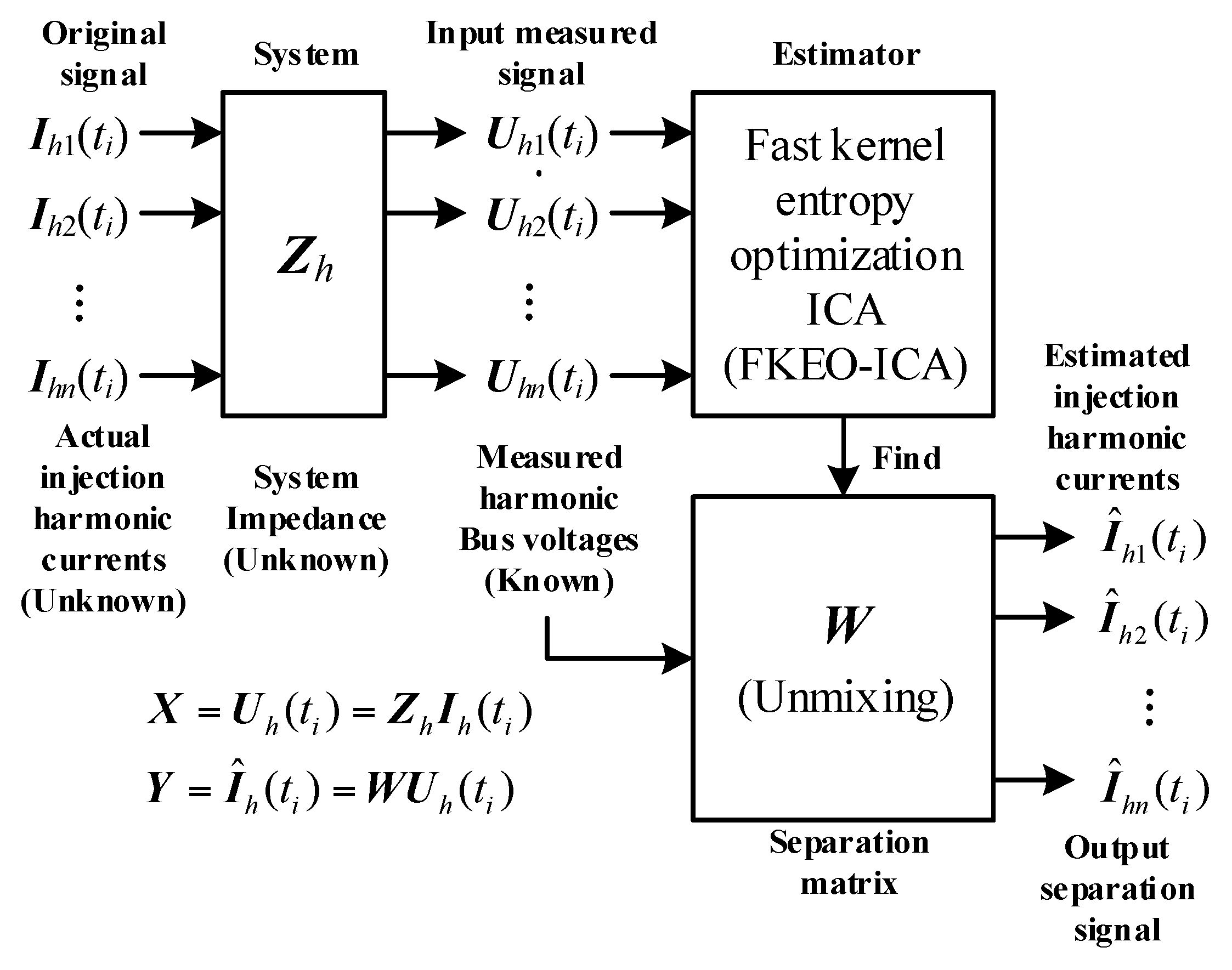
W so as to eliminate the mixing. That is, the estimation of the sources can be given as:
where
Y is the estimation value of
S.
In accordance with Equations (1) and (2), , , and in the HSE model are associated with , , and in the ICA model, respectively. Therefore, the harmonic state estimation problem can be formulated as an ICA problem.
3. The Principle of the FKEO-ICA Algorithm
In view of the high dimension and large sample size of harmonic data involved in the electric power systems, the fast kernel optimization ICA method based on the FFT-based fast convolution, as presented in [
20], is applied to estimate harmonic currents in this paper. The basic principle of the FKEO-ICA algorithm is described as follows.
The set of independent signal sources is denoted as , where represents each individual source, . With regard to the linear mixture of , the set of measured signals is denoted as . Additionally, is assumed to be the set of estimated sources.
According to Equation (3),
can be obtained. The aim of ICA is to calculate separation matrix
W which can make the estimated sources independent. The common criterion is the mutual information of the estimated signal sources [
14]. Furthermore, the mutual information of
is expressed as follows:
where
is the entropy of estimated signal
, and
is a constant, generally, which can be ignored in the optimization process. Accordingly, the minimization problem to be solved becomes:
where
is a constant weight,
is a weighted sum which is applied to solve the ambiguities issue from the scale invariance of mutual information, and its impact for the calculation accuracy is negligible [
20].
Based on Parzen-windows (PW), the estimation of
is capable of differentiating estimated entropies, while an approximate expression is required for the differential entropy gradients [
20]. For a given
r, the PW estimator for the probability density function is:
where
is sampled from estimated signal
and
represents the smoothing kernel function.
The PW estimator for
is:
The gradient of
is
[
16]. Thus, the gradient of
can be expressed as:
where
can be calculated from:
The derivatives of Equation (7) are:
where
represents the derivatives of
, and
represents the kroneker delta,
.
Based on the above-mentioned derivation process, the gradient equations have been converted into accurate analytical formulae, and the separation matrix
W can, thus, be obtained. Further acceleration based on the FFT-based fast convolution is described in [
20], which has proved that the estimation error is reasonably small. Moreover, through the FKEO-ICA algorithm, both high computational accuracy and low computational complexity can be achieved.
The harmonic current estimation model using FKEO-ICA is illustrated in
Figure 1.
4. Identification of Harmonic Source Localization Using Minimum Conditional Entropy
Similar to other ICA methods, FKEO-ICA is not capable of determining the exact bus of harmonic sources. The relationship between the harmonic currents and the bus voltages is
, which indicates that the injected harmonic current
produced by the harmonic source at the injected bus has a certain correlation with the bus harmonic voltage
. As a consequence, the bus harmonic voltage
and the injected harmonic current
can be considered as two random variables with associated distributions. In accordance with the information theory [
21,
22,
23], the conditional entropy has been employed to measure the correlation between two random variables in case one of them is known. The pair-wise conditional entropy between the estimated harmonic current
and the measured bus voltage
at each frequency can be expressed as follows:
where
is the joint probability distribution of the measured bus voltage and the estimated harmonic current;
, where
is the probability of the estimated harmonic current under the given measured bus voltage;
is the marginal probability distribution of the measured bus voltage averaging over information about the estimated harmonic current, and it can be calculated by summing the joint probability distribution over the estimated harmonic current.
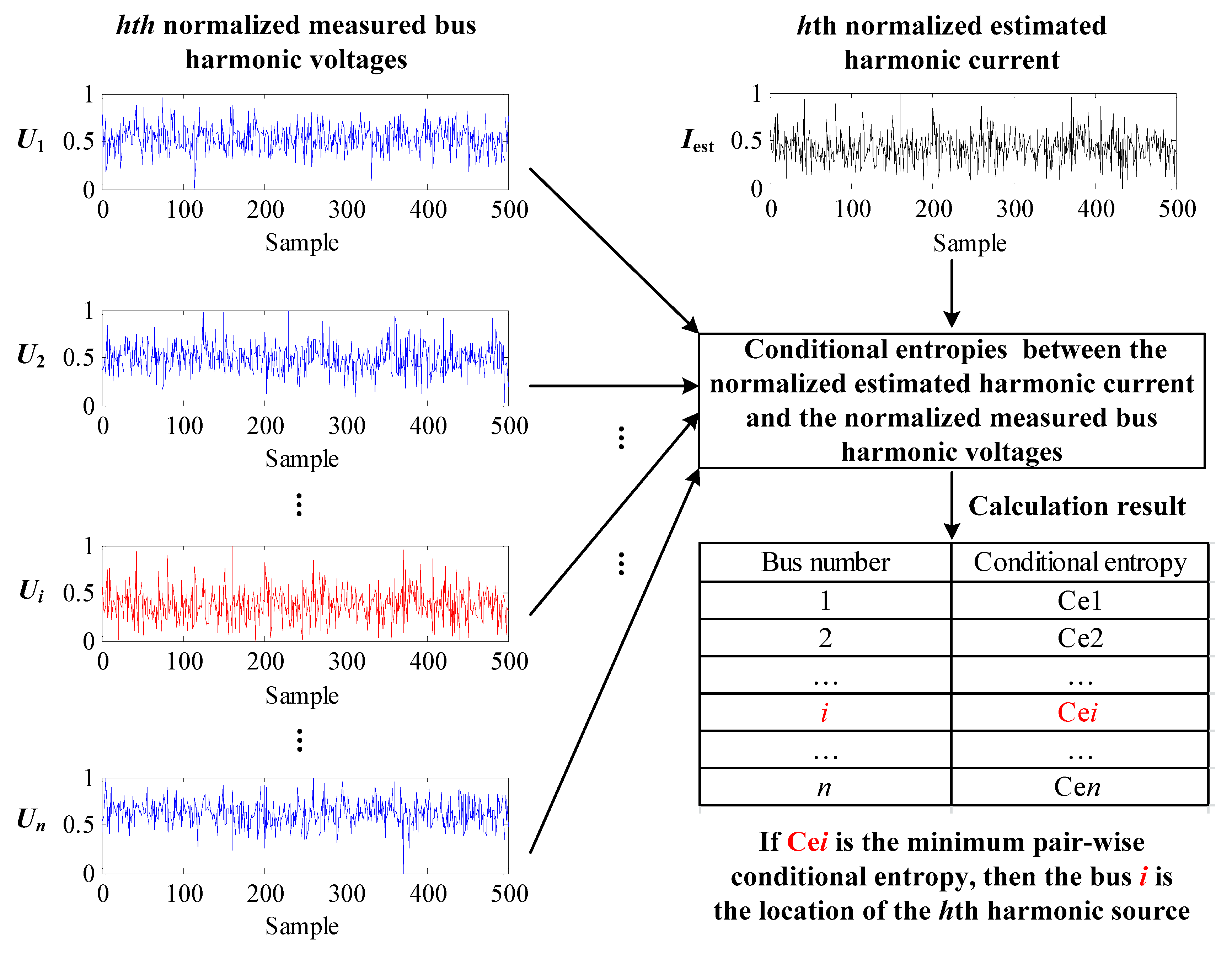
The stronger the correlation between the two random variables, the smaller their conditional entropy is. Owing to the current division effect between branches, the injected harmonic current has minimum conditional entropy with the voltage of its injected bus, compared with the conditional entropies with other bus voltages. Thus, The minimum pair-wise conditional entropy
can be used to determine the harmonic source location, where
is the normalized estimated harmonic current, and
is the normalized measured bus voltage. The principle of harmonic source localization based on the minimum pair-wise conditional entropy is shown in
Figure 2.
5. Harmonic Source Localization Using FKEO-ICA and Minimum Conditional Entropy
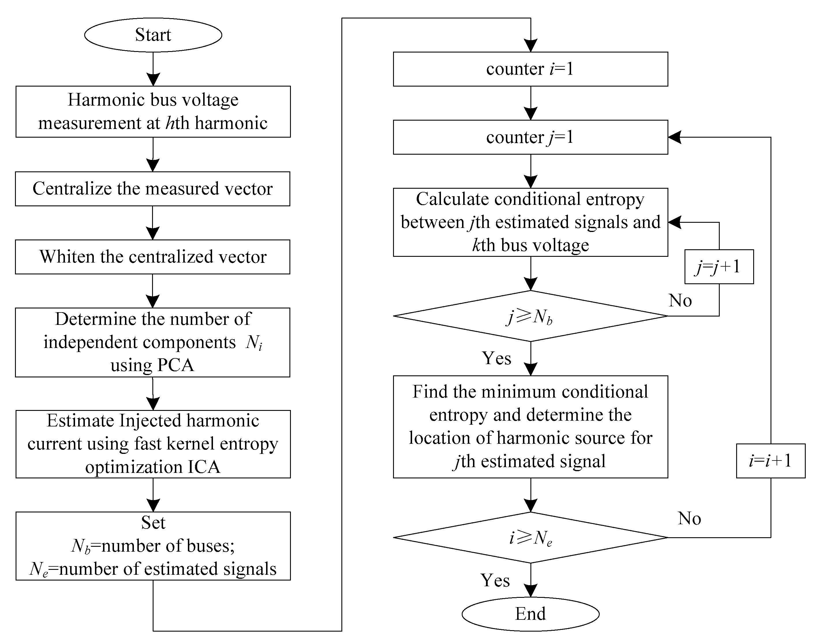
The process of the harmonic source localization based on FKEO-ICA and minimum conditional entropy is as follows:
(1) Measurement of bus harmonic voltages
The harmonic voltages at all buses are measured and represented as vector .
(2) Centralization of the harmonic voltage data
The first pre-processing procedure is centralization, which aims to transform vector into the zero-mean vector by subtracting the mean of .
(3) Whitening of the centralized data
The second pre-processing procedure is to whiten the centralized data. This means that the centralized vector
can be linearly transformed into
. In the process, the components of
are independent, while the variances of
are normalized into a unity. The linear whitening transformation can be defined as:
where
indicates the orthogonal matrix with vectors
as the unit norm eigenvectors of the covariance matrix relating to
, and
is the diagonal matrix of the eigenvalues concerned with the covariance matrix of
.
(4) Determination of the number of independent components
Prior to the estimation of harmonic currents, the number of independent components needs to be identified through the principal component analysis [
24].
(5) Estimation of harmonic currents
The FKEO-ICA algorithm elaborated in
Section 3 can be used to obtain the separation matrix
W. Then the harmonic currents
can be estimated based on Equation (3).
(6) Localization of the harmonic sources
The last procedure is to calculate the conditional entropies between the normalized estimated currents and the normalized voltages based on Equation (11), and find the precise location of harmonic sources based on the minimum conditional entropy.
In summary, the process of the proposed algorithm for harmonic source localization can be illustrated in
Figure 3.
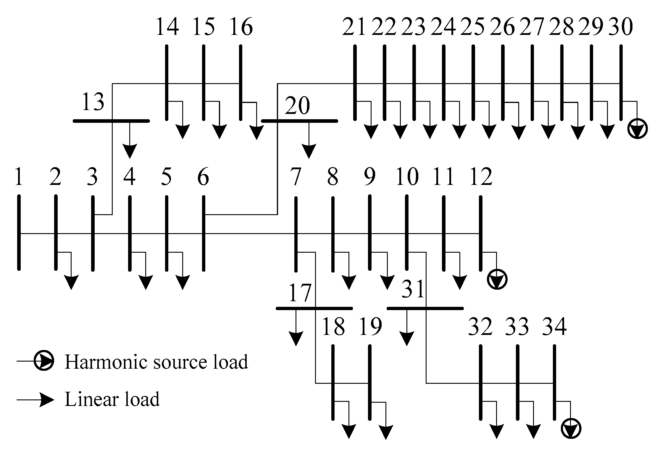
6. Example Test
The IEEE 34-bus power system [
25] as shown in
Figure 4 is selected as the test system, with the system parameters listed in the
Appendix.
In the simulation, the fundamental frequency of the system is 50 Hz. The harmonic loads are modeled as constant power loads in the fundamental frequency power flow calculations. Then the power flow solution, together with the spectrum of the six-pulse HVDC as shown in
Table 1, are used to obtain the harmonic current source models. In our work, the 5th, 7th, and 11th harmonics are selected for the test, as the amplitude of them is larger than that of the higher order harmonics. Then, the three harmonic sources containing the 5th, 7th, and 11th harmonic orders are located at bus 12, 30, and 34, respectively. To simulate altered operating situations, all loads are multiplied with the random variables, which are statistically independent and obey a Laplace distribution with the variance of 0.002. Furthermore, the Backward/Forward Sweep-based algorithm [
26] has been applied to calculate harmonic power flow and generate harmonic voltages. To take measurement noises into account, the white Gaussian noise with SNR = 60 dB is added to the harmonic power flow data using the “AWGN” function in the Communications System Toolbox of MATLAB. In this study, 600 samples of RMS harmonic bus voltages and injected harmonic currents for the 34 buses were created.
Comparison has been made among the estimation performances of FKEO-ICA, Fast-ICA [
17], equivalent robust ICA (ERICA) [
27], and unbiased qNewton ICA (UNICA) [
27]. All algorithms are implemented on MATLAB R2014a in an Intel Pentium Dual Core, 2.0 GHz, 1 GB RAM computer. The correlation coefficients (
CC) between the actual and estimated currents are calculated as shown in
Table 2. Meanwhile, the errors are measured by:
where
and
represent the estimated and actual current values under the same conditions of time and frequency, respectively;
MAE indicates the mean absolute error;
MSE indicates the mean squared error; and
MAPE indicates the mean absolute percentage error. The errors of four ICA algorithms are shown in
Table 3,
Table 4 and
Table 5.
The tables above show that, compared with other two ICA algorithms, the FKEO-ICA and the Fast-ICA algorithm can estimate harmonic currents more accurately. For all of the concerned frequencies, the correlation coefficients of the FKEO-ICA algorithm are closer to 1 compared with that of other ICA algorithms. Meanwhile, the error of the FKEO-ICA algorithm is relatively lower at all concerned frequencies, thus proving better accuracy of the FKEO-ICA algorithm compared with other ICA algorithms.
In order to test the running time of different ICA algorithms concerned with harmonic current estimation, simulations are conducted repeatedly 100 times. It can be shown in
Table 6 that the running time of all algorithms is around three seconds, while the proposed method can reach a higher estimation precision with a slightly longer time in comparison with other methods.
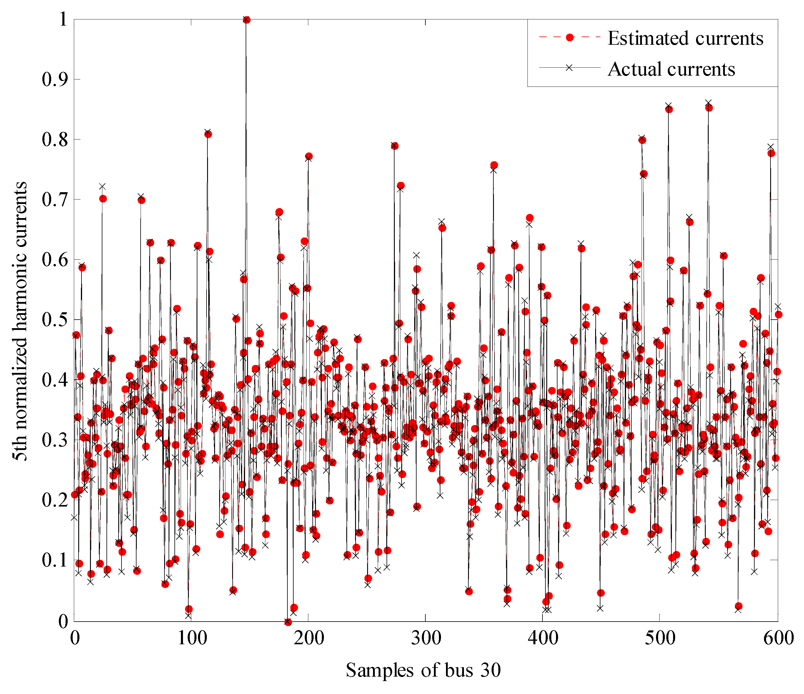
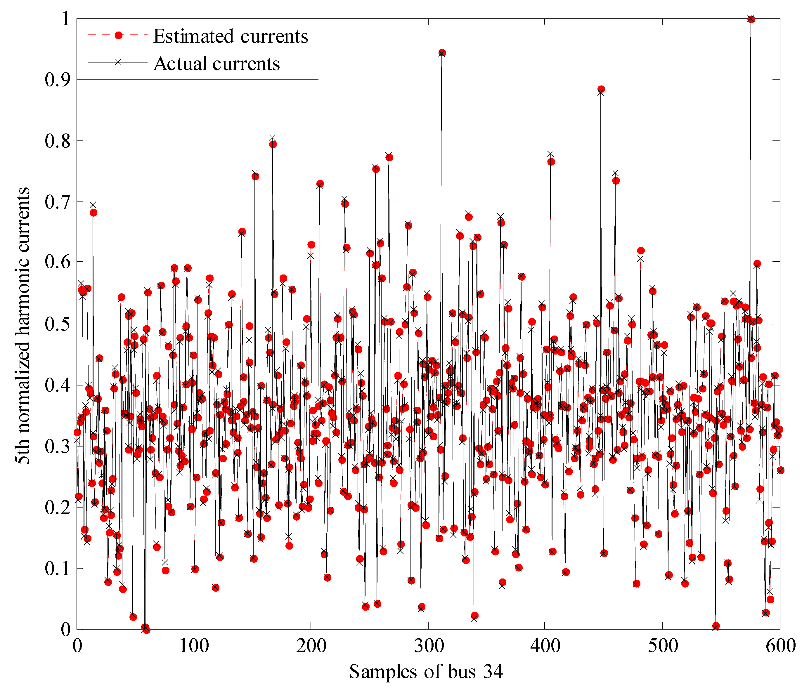
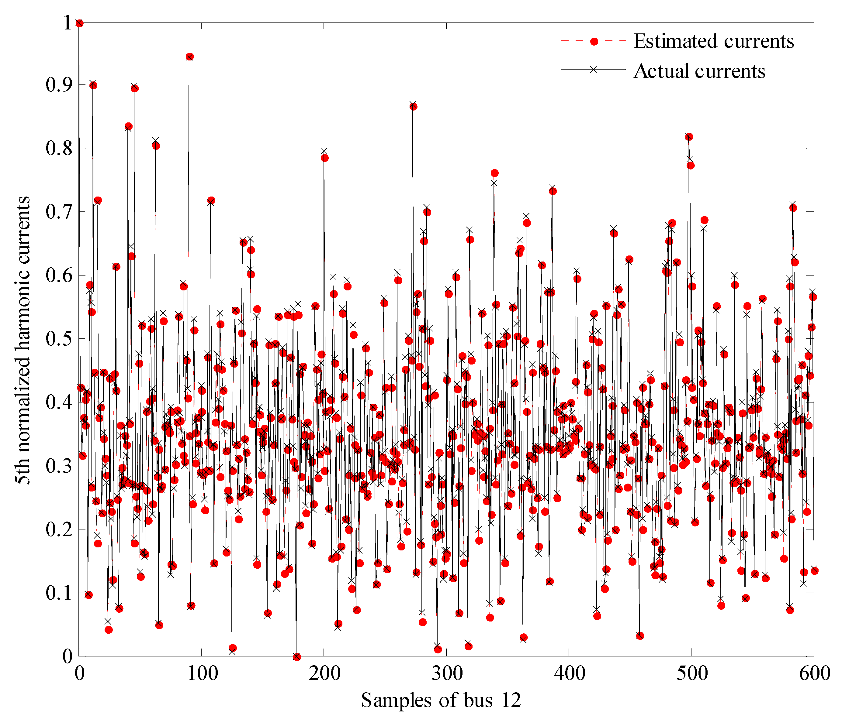
Based on the FKEO-ICA algorithm, the comparisons of normalized actual and estimated harmonic currents of bus 12, 20, and 34 at
h = 5 are shown in
Figure 5,
Figure 6 and
Figure 7, which indicate that the estimated harmonic currents are highly consistent with the actual harmonic currents.
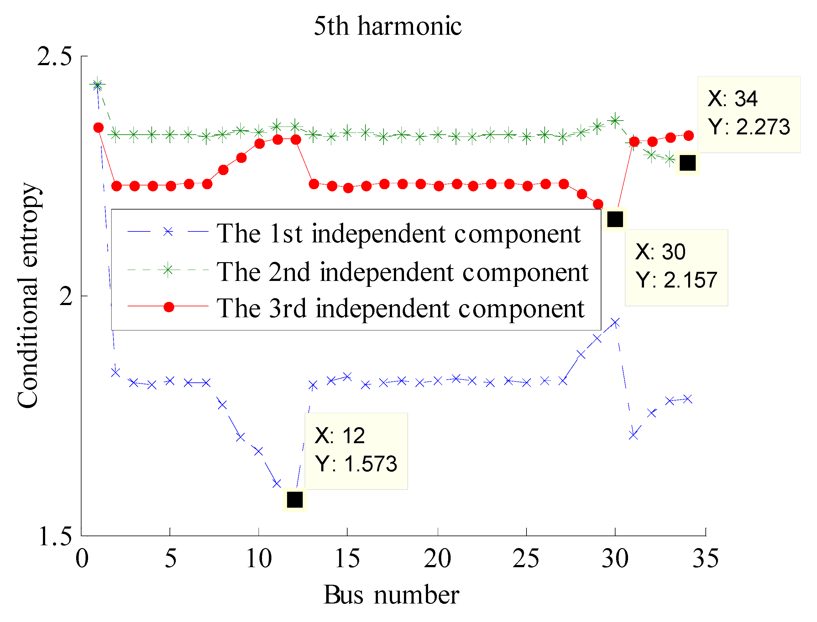
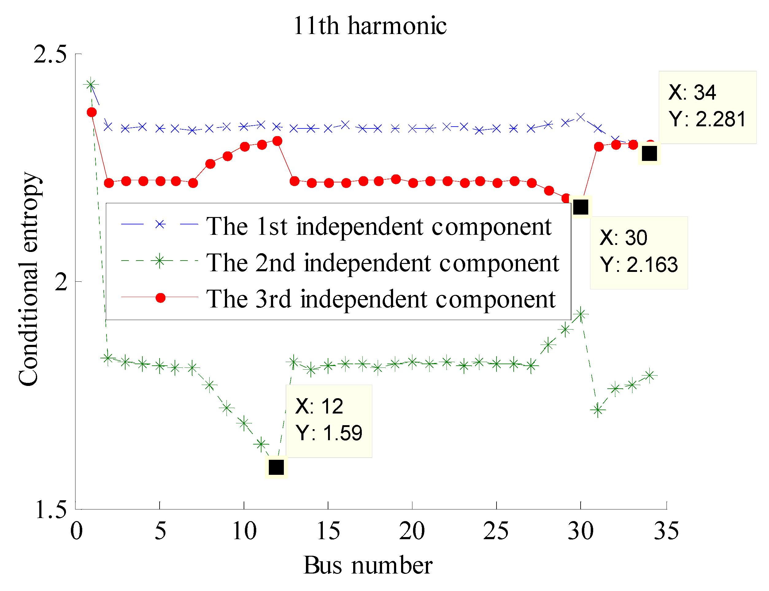
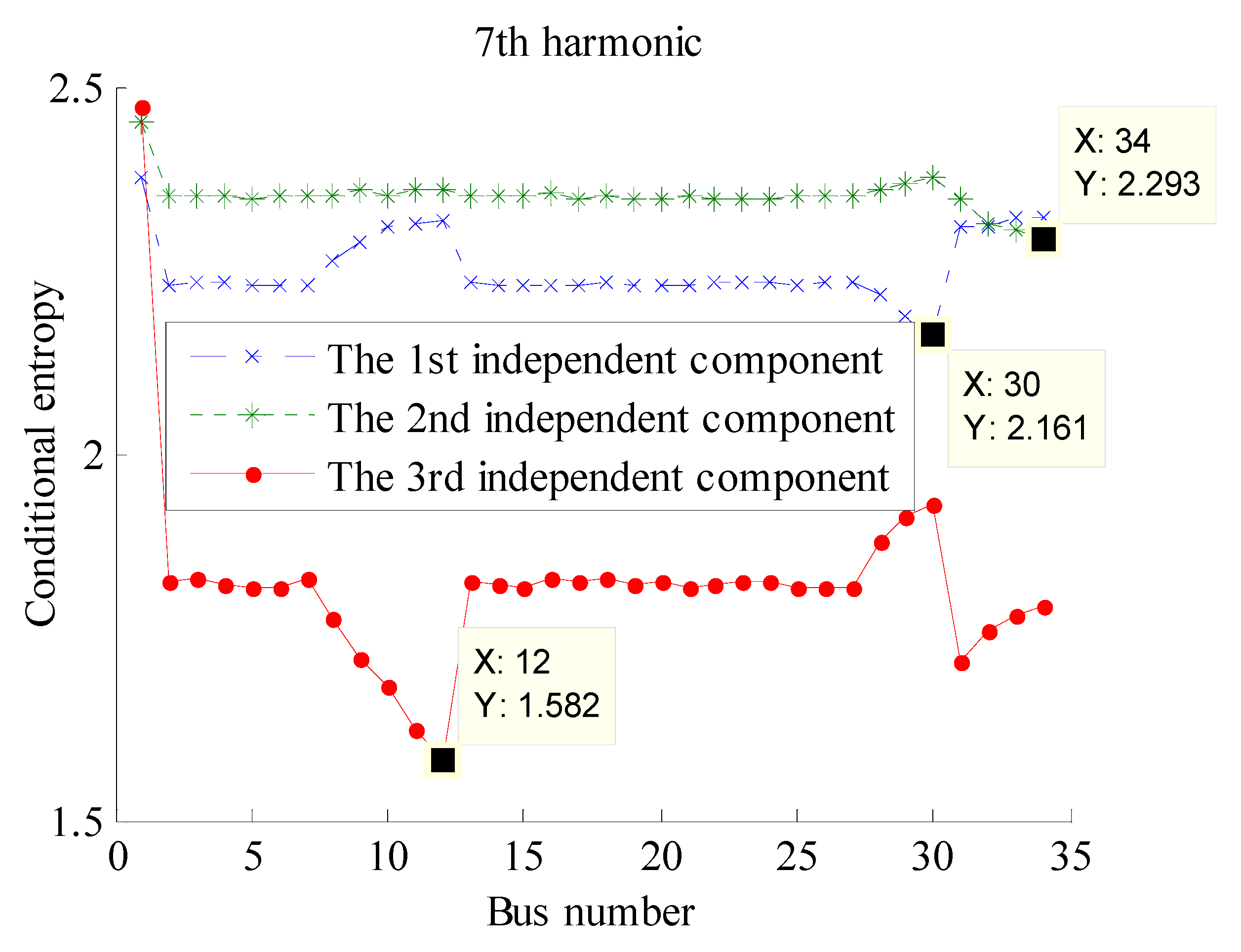
To find the exact bus position of harmonic sources, the pair-wise conditional entropy
is calculated for each concerned frequency. The results are shown in
Figure 8,
Figure 9 and
Figure 10, where the base of the algorithm in Equation (11) is assumed as 2.
As indicated in
Figure 8,
Figure 9 and
Figure 10, although the orders of the estimated independent components (
i.e., estimated harmonic currents) are random, the harmonic injection bus can be accurately identified when its voltage exhibits the minimum conditional entropy with the estimated harmonic currents.
7. Conclusions
This paper presents a method to identify harmonic sources based on FKEO-ICA and the minimum conditional entropy. In this study, the injected harmonic currents are estimated through the FKEO-ICA algorithm, in which the processed harmonic bus voltages are used as inputs. The advantage of the FKEO-ICA algorithm lies in that it does not require the prior information about system parameters. Additionally, the minimum conditional entropy is applied to locate the bus position of harmonic sources. The results indicate that the FKEO-ICA could achieve a better accuracy of harmonic current estimation, while the minimum conditional entropy can precisely locate the harmonic sources. In the simulations, only weak measurement noises are taken into consideration. In practice, the harmonic measurement quality and the detection technology can be further improved so as to avoid the increase of estimation errors caused by strong measurement noises.


