1. Introduction
Quantities of interest are typically surrounded by a number of uncertain events. According to statistical reasoning, probability measures are employed to model uncertain events and to make inferences over the quantities of interest. The observed relevant information is contained in the observed sample [
1]. The statistical model is formally written by the triplet:
, where
is the sample space,
is the associated
σ-field and
is a family of sampling probabilities indexed by a parameter
, where
, with
, is a non-empty set called the parameter space. The quantities of interest are connected with the parameter
, e.g., the expectation of some random quantity defined in the statistical model.
The inferential process about
involves a summary of the information provided by the observed
data using (minimal) sufficient statistics and their respective induced models that concentrate the statistical relevant information. There are essentially two types of estimation theories, namely, point and set estimation theories; this paper focuses on the latter. For the univariate case, Neyman [
2] provided a theory of confidence intervals, which is based on a random interval
such that its probability is greater than (or equal to) to a given predefined value
(confidence level), where
X is the random sample. The most frequent interpretation states that if the experiment is repeated and a confidence interval is computed for each experiment, then the parameter
θ is expected to lie at least in
of those observed confidence intervals. However, in practice, the experiment is repeated once and just one confidence set is observed. This observed confidence set
contains non-random values, since
x is the observed value of
X, so, the probability that this observed confidence set contains any specific point or region will always be zero or one [
3]. Therefore, after observing the sample the confidence sets cannot be interpreted in terms of frequencies (as Neyman proposed in 1935 [
2]).
Fuzzy set theory developed by Zadeh [
4,
5] allows generating possibility distributions by using confidence sets (see for example [
6,
7,
8]). Probability measures are dominated by possibility measures in the following sense: Events with zero possibility must have zero probability, however not all events with positive possibility have positive probability [
9]. That is, in some cases, some events with positive possibility do have zero probability. Therefore, possibility measures can provide an information not featured by probability measures. We will show that, for a given observed sample, the related possibility distribution provides information about the structure of confidence sets.
The main contribution of our paper is to show how to generate a fuzzy number from a given confidence set and therefore infer about some parameter
under the light of fuzzy set theory. Although this approach has already been discussed in the literature (see [
7,
8,
10]), our approach is more general (e.g., the confidence region is formally defined, the parameter space is multidimensional,
etc.) and oriented to the statistical community. In this context, the proposal presented in this paper is based on a general membership function proposed in Patriota [
11]. As a consequence of this characterization, properties and comparisons of confidence sets are discussed under the scope of fuzzy set theory but from a statistical point of view.
The paper is organized as follows. In
Section 2, a review of fuzzy set theory for statisticians is provided.
Section 3 focuses on the connection between confidence sets and fuzzy sets through a membership function.
Section 4 presents some examples of the results obtained and
Section 5 provides an application to a real dataset. Finally, in
Section 6, a discussion about different proposals existing in the literature for relating confidence theory and fuzzy theory is presented.
Section 7 ends the paper with some remarks and conclusions.
2. Preliminaries
2.1. A Brief Review of Fuzzy Theory
Fuzzy set theory provides mathematical treatment of some vague linguistic terms such as “about”, “around”, “close”, “short”, among others. From the fuzzy theory viewpoint, numbers are idealizations of imprecise information expressed by means of numerical values. For example, when the height of an individual is measured, a numerical value is registered including some inaccuracies. Such inaccuracies may have been caused by the measurement instruments, human limitations, rounding, or biased prior information among many other causes. If the “real" value of the height is represented by the number
h, maybe it would be more correct to say that the value of the height is approximately and not exactly
h [
12], the word “approximately” is imprecise and can be modeled by fuzzy theory. As was noted by Coppi
et al. [
13], fuzzy theory can provide an additional value to statistical methods because of the uncertainty inherent to the observable world and its associated information sources are combined beyond the traditional probability theory. For example, Tanaka
et al. [
14] introduced the concept of fuzzy regression while Wünsche
et al. [
15] characterized the least squares method for fuzzy random variables and Arabpour and Tata [
16] developed some theoretical elements regarding parameter estimation in fuzzy regression models. The connection between the estimation of parameters and fuzzy theory has been studied by several authors. Geyer and Meeden [
17] established a relation between the concept of
p-value and fuzzy structures and Parchami
et al. [
18] introduced the concept of fuzzy confidence intervals. On the other hand, Casals
et al. [
19] studied fuzzy decision problems by relating the concepts of hypothesis testing and fuzzy information nature. Saade and Schwarzlander [
20] and Saade [
21] proposed a characterization of fuzzy hypothesis testing while Watanabe and Imaizumi [
22] related the concepts of hypothesis test statistics and fuzzy hypotheses. Arnold [
23,
24] related the concept of fuzzy hypothesis testing with conventional methods of real
data analysis. Taheri and Behboodian [
25] generalized the Neyman–Pearson approach for hypothesis testing under the fuzzy point of view and Filzmoser and Viertl [
26] introduced the concept of fuzzy
p-value for statistical hypotheses using fuzzy
data. Recently, Patriota [
11] provided an evidence measure for testing null hypotheses that is intrinsically related to fuzzy theory.
2.2. Overview of Fuzzy Theory
In order to make our paper self-contained, we provide an overview of fuzzy theory in this section. We only use some concepts and terminology of fuzzy set theory, mainly based on the works of [
5,
27,
28].
Definition 1. Let be a non-empty subset of the k-dimensional Euclidean space. A fuzzy set is a set of ordered pairs , where is called the membership function for the fuzzy set . In addition, the empty fuzzy set is characterized by for all .
The fuzzy set theory extends the traditional set theory by relaxing the concept of membership of elements in their respective sets. On the one hand, in the ordinary set theory it is considered that (membership one) or (membership zero), that is, it is a binary operation. On the other hand, fuzzy set theory considers a degree of membership that ranges over the interval , that is, is a member of A with a certain degree and this same element is a member also of with another degree. Probability theory is built on the usual set theory and provides a number in to describe the degree of uncertainty that .
The main difference between probability theory and fuzzy theory lies in the definition of a set: the former considers traditional sets and the latter considers fuzzy sets. As will be seen in this section, the properties of fuzzy sets are very different from those of traditional sets. The applicability of fuzzy sets is enormous in language modeling [
29], image analysis [
30] among many others. One simple example is that an object with gray color has a degree of blackness and a degree of whiteness, so it would be much more informative to model this phenomenon inside the fuzzy set framework setting membership degrees than by setting a binary membership (traditional set theory).
From Definition 1, we can represent an ordinary set by using fuzzy notation. For instance, if , then any usual subset is represented by setting for all and for all . As a special case, let and be an interval on the real line with . Then, B can be written in terms of a fuzzy set as .
It is important to stress that membership and probability density functions are intrinsically different. For example, if is a density function, i.e., for all and , then we can obtain a membership function by defining , provided that . However, the converse is not necessarily true, since a membership function does not need to be integrable over Ω.
For probability density functions, it is common to define a support to characterize the set of all points with positive density. For membership functions, we have the same definition to represent the set of all points with positive membership in the fuzzy set. Definition 2 formalizes this concept.
Definition 2. The support of a fuzzy set
is defined as
Notice that, an element has full membership in its respective fuzzy set when its membership is one. In this context, the element fully contains all features required by the fuzzy set. Definition 3 formalizes the set of all points with full membership, that is, all points where their membership functions are equal to one.
Definition 3. The core of a fuzzy set is defined as .
When the core has as least one element, we have a normal fuzzy set (see Definition 4).
Definition 4. A fuzzy set is called normal if its core is nonempty. In other words, there is at least one point with
Let
be a normal fuzzy set. Then, the closer
is to one, the more we believe that
lies in
and the closer
is to zero, the more we believe that
is not in
. That is, the degree of membership for an element can also be seen as a measure of uncertainty [
29].
Let
and
be two fuzzy sets with membership functions
and
, respectively. According to Zadeh [
5], (see also [
31]), if
the common operations are defined as follows:
for all .
for all .
is the complement of for all .
for all .
for all .
From the above definitions, if we consider
as the universal fuzzy set, then for any fuzzy set
we have
, provided that the membership function of
has domain Ω. In addition, if there exists
such that
we have that
. Also, if there exists
such that
, we have that
. As the reader can see, these properties block the excluded middle and contradiction laws of classic set theory (for further details see [
31,
32,
33]).
The concept of a fuzzy set is very broad and difficult to handle without some additional specifications. In this context, the next definition allows us to specify fuzzy numbers, which are natural extensions of traditional numbers. However, this latter definition depends on fuzzy convexity, which is defined next (see [
5] for more details).
Definition 5. A set is convex if and only if for all and
Note that the concept of convexity under the fuzzy approach differs from the classic definition of convexity under functional analysis. More discussion about this concept will be presented in
Section 3. A fuzzy interval
is a fuzzy set that satisfies the condition of convexity and normality, so the core of a fuzzy interval is constituted by all elements with membership one. A fuzzy interval
is a fuzzy number when the cardinality of
equals 1 [
28]. Fuzzy numbers and fuzzy intervals are useful to represent imprecision for point and interval measures, respectively. As mentioned earlier, these concepts have multiple applications, e.g., in artificial intelligence, image processing, speech recognition, biological, and medical science, operations research, decision analysis, information processing, economics, geography, psychology, linguistics,
etc. More applications can be found in [
34,
35].
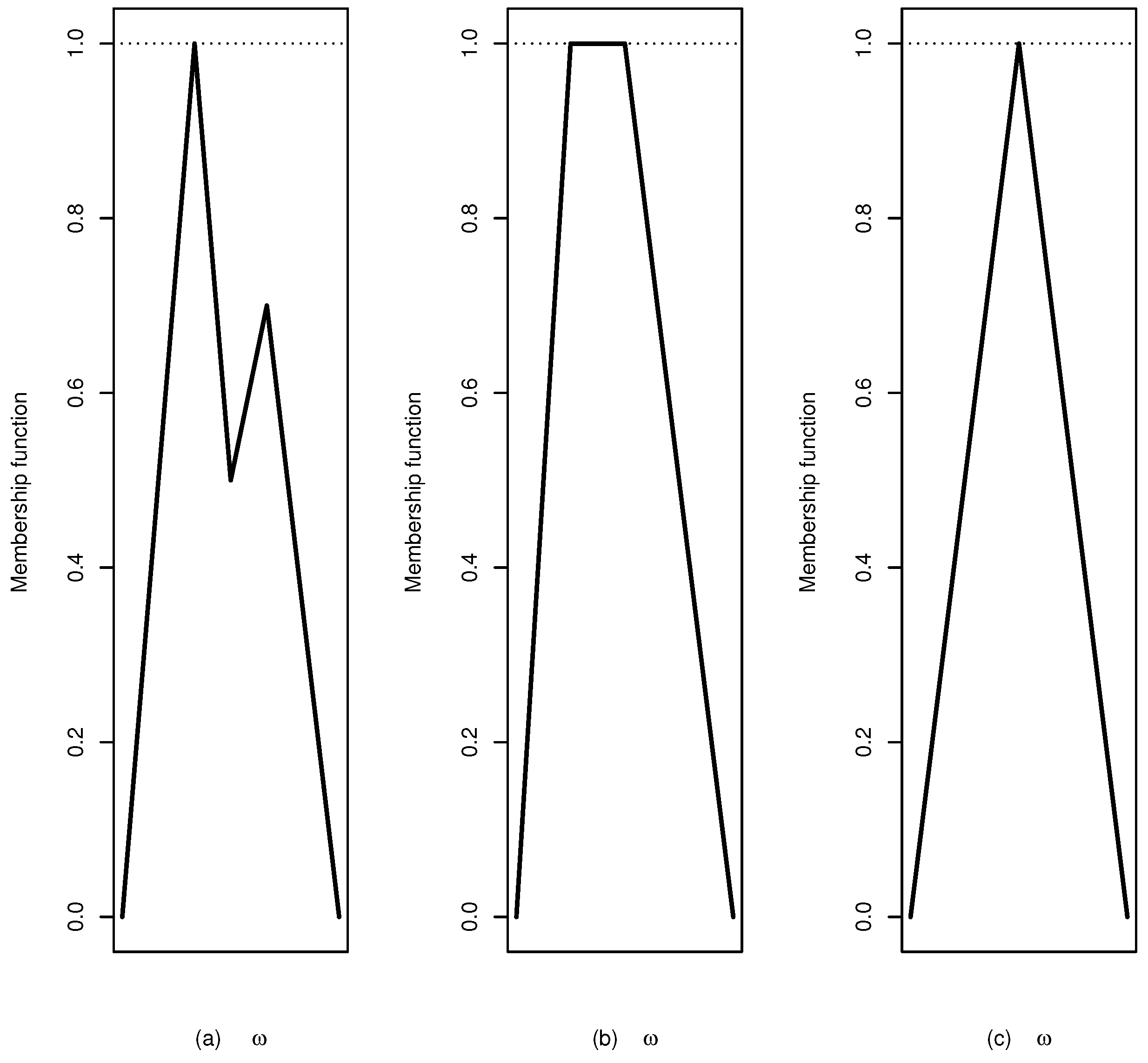
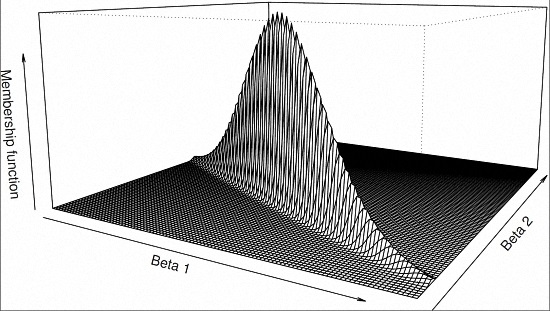
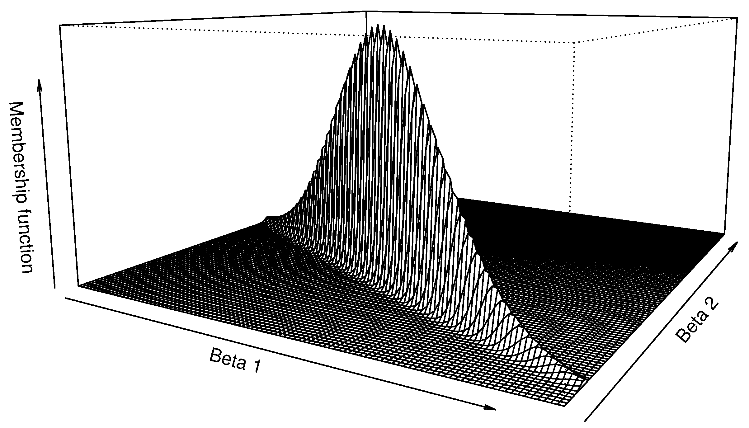
Figure 1a–c illustrate a general fuzzy set, a fuzzy interval and a fuzzy number, respectively.
Dubois
et al. [
27] defined the class of LR (left and right) membership functions defined over
,
i.e., the class of membership functions that can be entirely characterized by three parameters, namely,
, and two functions
L and
R. The next definition is related to the concept of LR-type fuzzy numbers.
Definition 6. The fuzzy number
is said to be of LR-type if two decreasing functions exist
with
and positive real numbers
,
,
such that
where
m is called the center of
and
α and
β are called the left and right propagations, respectively.
If , is called a symmetric fuzzy number. For a symmetric membership function, the equality holds for all .
In this paper, we use all definitions presented in this section to connect the classic statistical quantities with fuzzy theory.
3. Confidence Sets and Membership Functions
As mentioned in the Introduction, the main goal of this paper is to infer about some parameter using the confidence sets under the fuzzy set theory. For that reason, we start this section by presenting the definition of a general confidence set.
Under a parametric statistical model
with
, where
and
, a
confidence set is a function
, where
is the family of all subsets of Θ (the power set) satisfying
for every
, where
is a random vector defined in the statistical model (see [
36], p. 315). When
for all
, then the confidence set
is exact. Procedures to build confidence sets can be found in [
37,
38,
39,
40,
41] among others. These procedures are in general based on pivotal quantities and likelihood-ratio statistics. Here,
is called the confidence level and
α is called the significance level [
42]. Intuitively, the interval width depends on the confidence level, for instance, the greater the confidence level the greater the interval width built under normal distributions (see [
43]).
After observing the sample, the confidence set
is a fixed set and
is zero or one, where
is the observed sample, so the probability statements in Equation (
1) are used just to construct a proper confidence set. Once the sample is observed, this confidence set is fixed. Therefore, the observed confidence sets cannot be interpreted in terms of probabilities (see [
44] Section 3.1.2, p. 41, for further details). In this section we show that, although it is not possible to make probabilistic statements about observed confidence sets, we can interpret the observed confidence sets in terms of fuzzy sets. We present a general membership function that provides all information contained in an observed confidence set
, for all levels
(alpha-cuts).
Lemma 1. Let be a confidence set of level for some subset of Θ
, where . Let where is non-empty. For each , we definewhere . We use the short notation when the family is not the focus. Then, is a membership function, that is, . Proof. As is a function and is non-empty. The proof is straightforward. ☐
For each proposed confidence region, we can represent the parameter space by the fuzzy set
where
is given in Equation (
2). Note that for different confidence sets
and
we have different memberships, namely
and
, respectively, where
and
with
. As a consequence, the resulting fuzzy sets will have different representations, namely
respectively. Additional information with respect to Equation (
2) can be found in Mauris
et al. [
45] and more recently in [
11]. Patriota [
11] studied some relationships with p-values when the confidence region
is built under the likelihood-ratio statistic.
The next result characterizes the core of .
Theorem 1. Let and be the quantities defined in Equation (2), then . Proof. From Definition 3, we have that . Now, we have that if, and only if, . This last fact occurs when for all concluding the proof. ☐
Theorem 1 characterizes the functional form of the core for the membership function defined in Equation (
2), that is, those values in Θ that produce full membership.
Remark 1. If the confidence set is centered in the maximum likelihood (ML) estimate , then we have that . This means that the ML estimate is part of the core of the fuzzy set . We can interpret as the set of all parameter values for which the related probability distribution explains the observed data according to .
Next we define non-increasing confidence sets in terms of the significance level α.
Definition 7. Let be a family of confidence sets. We say that is a non-increasing family of confidence sets if for all .
The next result relates the monotonicity property of confidence sets with the membership functions.
Theorem 2. Let be a family of non-increasing confidence sets. If , then , for all and , where and with .
Proof. As
and
is non-increasing, we have for each
and
that
Applying the supremum, we obtain
, concluding the proof. ☐
Another important result for non-increasing confidence sets is the relationship between the convexity concept in Definition 5, defined by Zadeh [
5], and the monotonicity property. This relationship is based on Theorem 2, concluding that
, for all
and
and therefore
is convex in the fuzzy context. Theorem 2 can be used to compare the membership functions. Next definition introduces the concept of supremacy for comparing confident sets.
Definition 8. Let be two membership functions with the same core. We say that has total supremacy over if for all . They are totally equivalent if for all . We denote total supremacy by and total equivalence by .
Definition 8 allows us to compare two different confidence sets, e.g., we can determine if a confidence set is more conservative than another for all confidence levels. Definition 8 is similar to the definition of
superiority given by Xie and Singh [
46]. Note also that if
is the family of all membership functions then
establishes an order relation in
and this relation is the order relation of the inclusion for fuzzy sets, (see for instance [
47]). Notice that Definition 8 is strong and is not applicable in many situations, notably if two membership functions have different core sets. In order to make the supremacy concept less restrictive, allowing us to include more situations, we define the following operators.
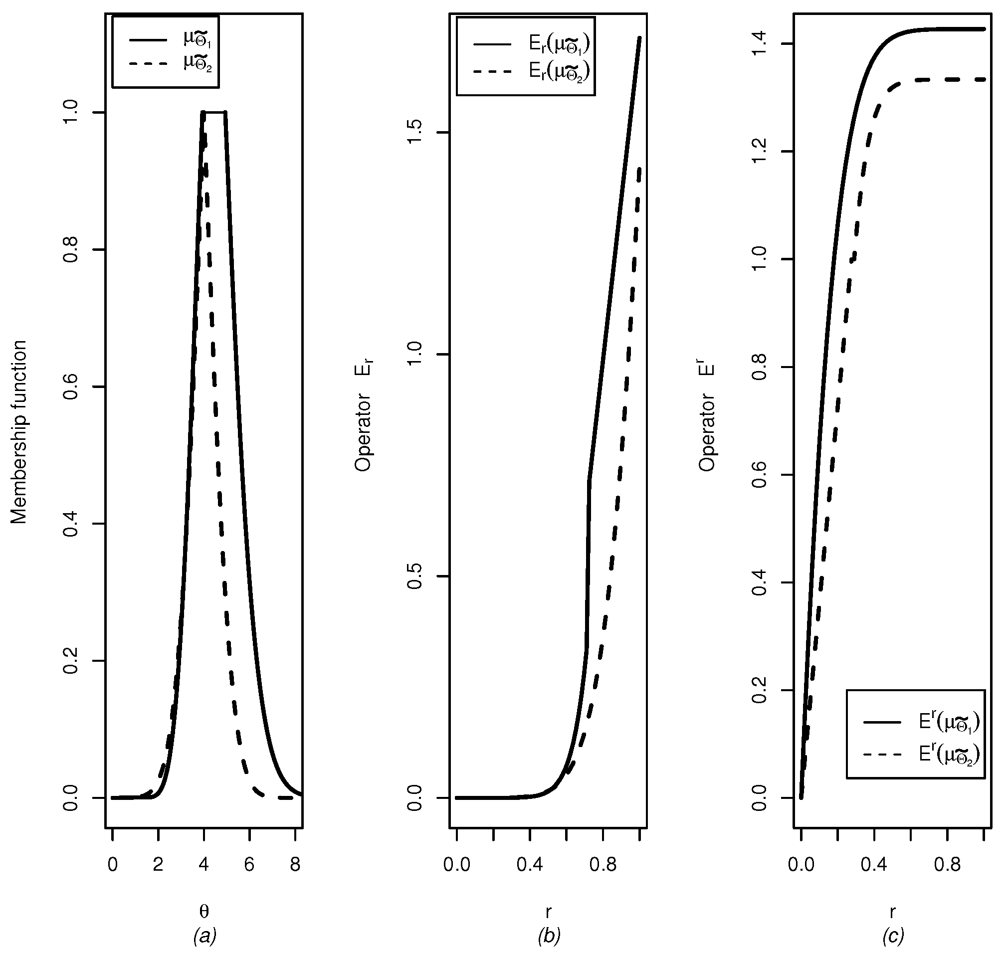
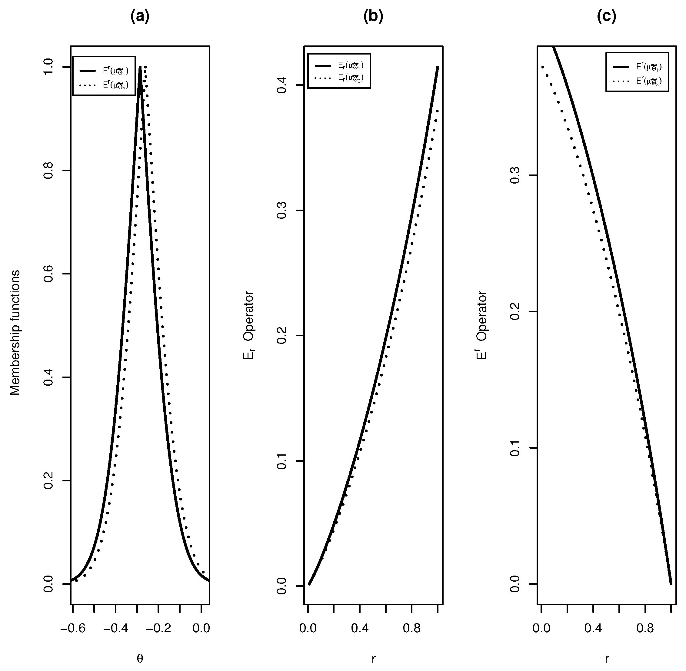
Definition 9. Let
and
two continuous membership functions. We say that
has
r-up-supremacy over
if
, and is denoted by
. Moreover, they are
r-up-equivalent when
, and are denoted by
, where
with
and
is such that the resulting integral is well defined.
If
is integrable with respect to the Lebesgue measure in dimension
,
has
r-down-supremacy over
if
, denoted by
. Moreover, they are
r-down-equivalent when
, and it is denoted by
, where
with
We call the r-up integral operator and the r-down integral operator.
Notice that, if
is integrable, then by Definition 9, it is straightforward that
for all
. In addition, if
, we also have that
. Example 1 describes how to analytically compute the quantities
and
. However, for more complex models, analytical solutions are virtually impossible, so these integrals have to be computed numerically by using any software (for instance,
MAPLE,
MATLAB,
Ox,
R,
SAS).
Example 1. Let
be a random sample (the random variables are independent and identically distributed) from a normal population with mean
θ and known variance
and let
be the observed sample. Here,
and a
confidence set for
θ, using the pivotal quantity method, is given by
for
, where
is the sample mean and
is the
qth-quantile of a standard normal distribution. The membership function is given by
Then, solving the equations
with respect to
and
, where
, we obtain
and
where
. Letting
, we have that
Now, by using the identity [
48]
where
stands for the standard normal density function, we have that
Similarly for the
r-up integral operator,
then
Definition 9 will be used to identify more conservative confidence sets. It is possible to show that , and satisfy the requirements to be order relations (reflexivity, antisymmetry and transitivity) and , and satisfy the requirements to be equivalence relations (reflexivity, symmetry and transitivity).
Theorem 3 establishes some relations among the three types of supremacies.
Theorem 3. Let be two continuous and integrable membership functions. Then,Moreover, if ,where . Proof. Let and and define . Notice that , for all , if and only if there exist and such that , where the latter is the inclusion of fuzzy sets and depends on the membership function . This implies that for all . The proof of the converse is similar. If , by the equality of the cores, we have if and only if . ☐
A confidence interval is said to be more conservative than another if the former interval’s amplitude is greater than the latter’s for a specific significance level. A procedure to generate a confidence interval is considered more conservative than another if the interval’s amplitude is greater than the latter’s for all significance levels. Below, we define the conservative concept for general confidence sets.
Definition 10. Let and be two families of confidence sets. We say that is more conservative than if their respective memberships and satisfy for all . We say that the region is up-more conservative than if and down-more conservative if .
The next proposition establishes some properties of . The proof is straightforward from Lemma 1, Definition 3 and Definition 8 and therefore is omitted.
Proposition 1. Let with as in Equation (2). Then, the following statements are valid.- 1.
, where . Also, if is a singleton then is a fuzzy number.
- 2.
If the cardinality of is greater than 1, then is a normal fuzzy set.
- 3.
If , then .
- 4.
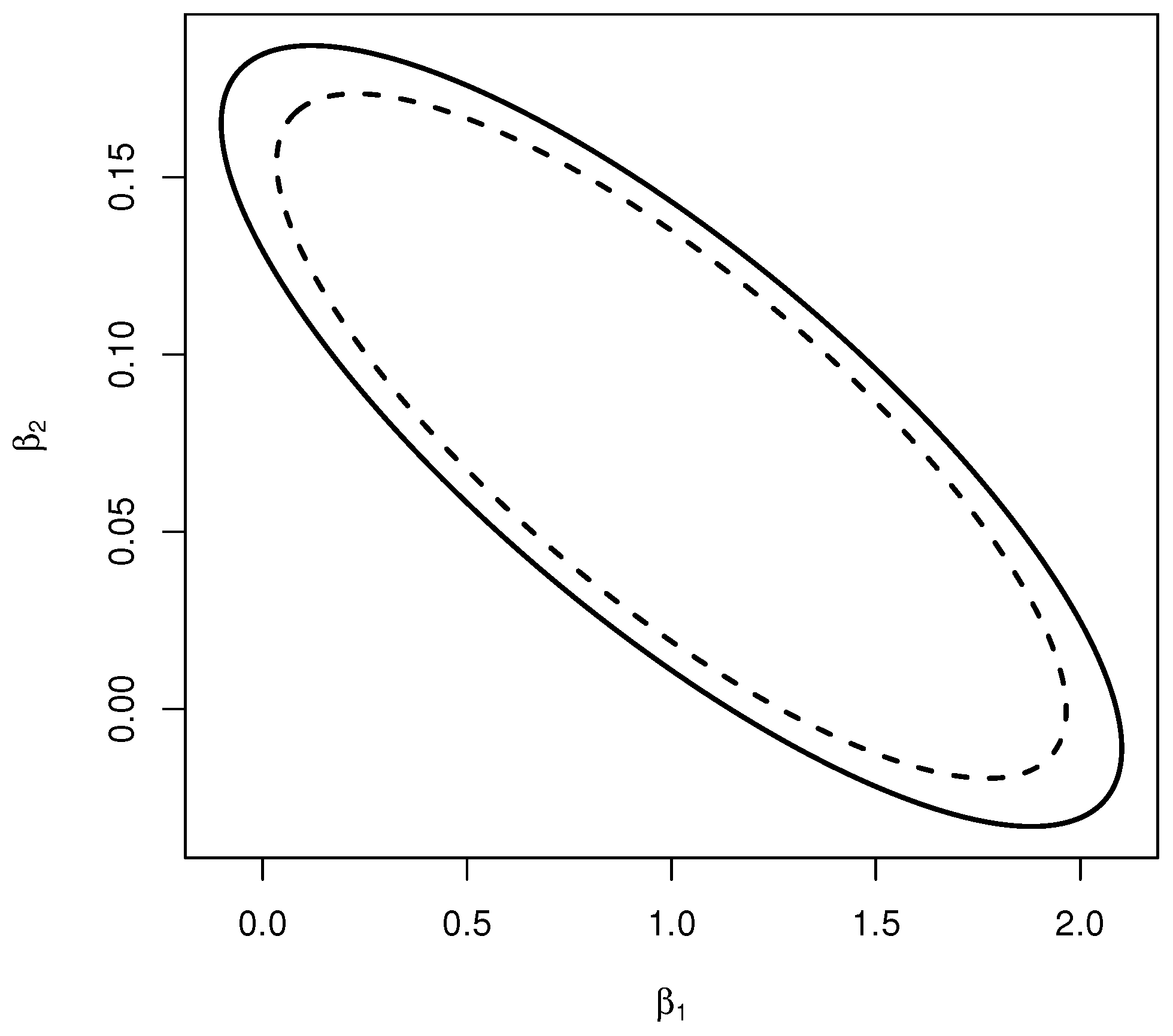
Let and be two fuzzy set representations over the parametric space Θ associated with and respectively. If for all , then and is more conservative than for all .
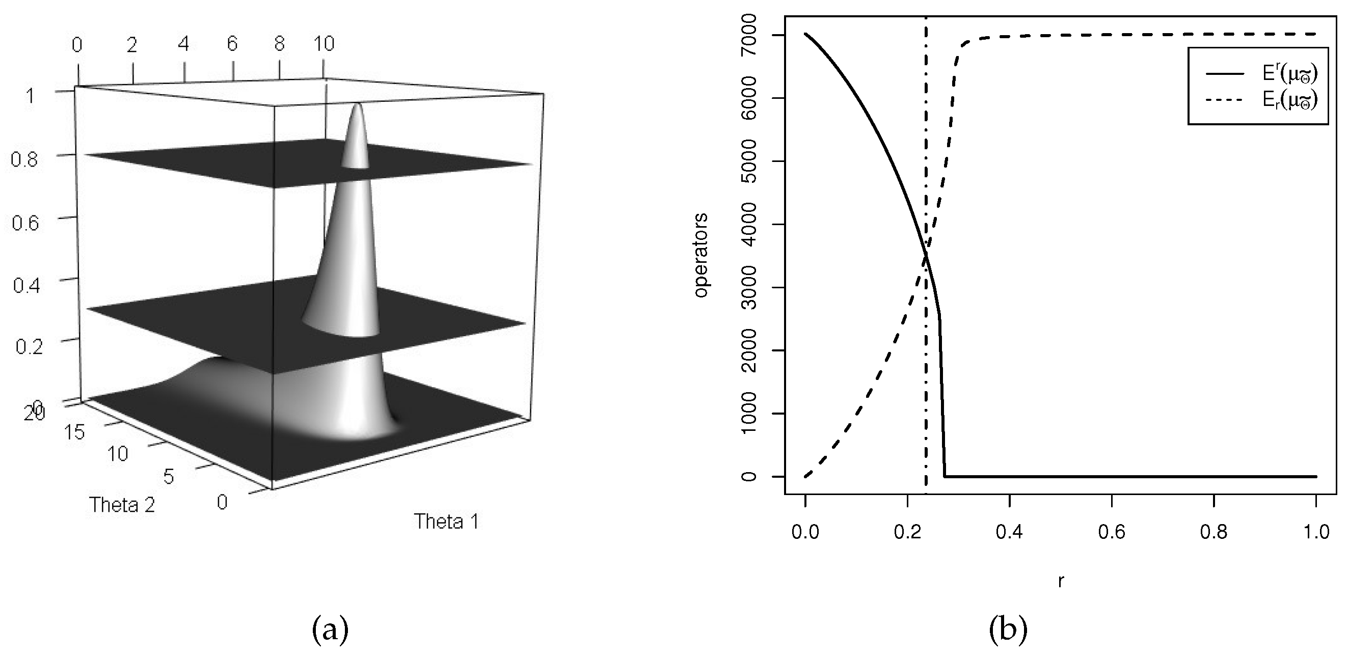
Definitions 8–10 are tools for comparing confidence sets through their respective membership functions. The membership functions used are defined in the same parameter space. However, there are situations in which we are interested in comparing confidence sets from a partial vector parameter with confidence sets from a full parameter vector. Therefore, a membership function for partial parameter vectors is defined next.
Let
, where
and
are vectors with dimensions
and
with
. Without loss of generality, let
be a confidence set for
and let Λ be the set in which
varies. Then, a membership function for
can be defined simply by
such that
The same properties of the membership (
2) and the above definitions are valid for this partial membership function.
6. Discussion
The connection between confidence sets and fuzzy theory has already been investigated in the fuzzy literature. As mentioned, some works about this topic have been published in recent years (see for example among others [
6,
7,
8,
10]). All of them are related to the idea of generating a possibility distribution from the information provided by confidence sets. The main goal of this proposal is to find, in the context of fuzzy theory, more information in terms of degrees of possibility about the parameter of interest. More information can be extracted from confidence sets (or confidence intervals) after the sample is observed than just one fixed set (or interval). Indeed, a large family of sets is available.
There are also other proposals with the purpose of inferring about a parameter using confidence sets. These proposals are the fiducial inference [
61], Dempster–Shaffer (DS) calculus [
62], confidence distribution [
46] and posterior Bayes. Some of them are carefully discussed by [
63,
64,
65]. The main idea of fiducial inference is to consider a distribution for a parameter of interest using the sample information. The idea is to provide some probability statements about a parameter from the observed information, particularly, the information provided by a sufficient statistic. Fiducial distributions are often criticized because in some cases they do not integrate to one,
i.e., they are not proper probability distributions [
66,
67]. Moreover, some pivotal quantities used to build a fiducial distribution generate inconsistent results [
68,
69,
70]. Therefore, some alternatives have been proposed such as confidence distributions and DS calculus.
The idea of confidence distributions is closely related with the fiducial distribution. As Schweder and Hjort [
71] established, “confidence distributions are the Neymanian interpretation of Fisher’s fiducial distributions” and they can be defined as a sample-dependent distribution able to represent confidence of all levels for a parameter of interest [
46]. One of the most famous representatives of this class of distributions is the bootstrap distribution. It is important to remark that, the confidence distribution is considered a distribution estimator and its interpretation has to be done in a frequentist framework, considering a fixed and non-random parameter. Moreover, it is possible to obtain confidence intervals, point estimates and hypothesis test results about the parameter of interest using this distribution.
The DS calculus is based on the idea of convert observed data and pivotal relationships to upper and lower probability statements [
72]. These statements are related to the probability of support by some subset of the parameter space, the contradiction of this event and the probability of “do not know" about both of them. According to Hanning and Xie [
72], a confidence distribution can be formally put into a DS framework. The main difference between DS calculus and fiducial and confidence distributions is the concept of
degree of belief. While the latter are focused on providing an estimator of a parameter of interest in terms of a quantity or/and interval/subset, DS calculus is concentrated on obtaining different degrees of belief or confidence for a simple question (related to a parameter). For this purpose, a
belief function is used rather than probabilities.
In Bayesian inference we use the concept of prior distribution over the parametric space in order to infer about the parameter of interest. Although in this case, a distribution is also obtained, the notion of unknown parameter considered in the approaches described above is replaced by the notion of random parameter. Moreover, in this setup, the prior distribution summarizes the available information about this parameter. Some other authors have comprehensively discussed the methods discussed in this section. For a detailed discussion, we refer to [
73,
74,
75].
Finally, our proposal intends to use the fuzzy set theory to represent a confidence set and, in this context, to provide more information to the statistical community about a specific confidence set. We believe, this approach represents both the uncertainty and imprecision existent about the parameter of interest by using the possibility theory obtained from a simple confidence set.


