General Bulk-Viscous Solutions and Estimates of Bulk Viscosity in the Cosmic Fluid

Abstract

We derive a general formalism for bulk viscous solutions of the energy-conservation equation for $\rho (a,\zeta )$, both for a single-component and a multicomponent fluid in the Friedmann universe. For our purposes, these general solutions become valuable in estimating the order of magnitude of the phenomenological viscosity in the cosmic fluid at present. $H\left(z\right)$ observations are found to put an upper limit on the magnitude of the modulus of the present-day bulk viscosity. It is found to be ${\zeta }_0\sim {10}^6$ Pa·s, in agreement with previous works. We point out that this magnitude is acceptable from a hydrodynamic point of view. Finally, we bring new insight by using our estimates of ζ to analyze the fate of the future universe. Of special interest is the case $\zeta \propto \sqrt{\rho }$ for which the fluid, originally situated in the quintessence region, may slide through the phantom barrier and inevitably be driven into a big rip. Typical rip times are found to be a few hundred Gy.

1. Introduction

Recent years have witnessed a considerable interest in theories of the dark energy cosmic fluid in the late universe. With present time defined as $t=0$, this means the region $t>0$. The interest in this topic is very natural, in view of current observations of the equation of state parameter, commonly called w. From the 2015 Planck data, Table 5 in [1], we have $w=-{1.019}_{-0.080}^{+0.075}$. Writing the equation of state in the usual homogeneous form:

$$p=w\rho ,w=\mathrm{constant}\equiv -1+\alpha ,$$

(1)

with the parameter w here assumed constant for simplicity, we see that the value of α lies between two limits,

$${\alpha }_{\min }=-0.099,{\alpha }_{\max }=+0.056.$$

(2)

It is thus quite conceivable that the cosmic fluid can be regarded as a dark energy fluid (the region $-1<w<-1/3$ is called the quintessence region, while $w<-1$ is the phantom region). Observing that the dark energy fraction is so dominant, about $70\%$, it has, for the future universe, been common to describe the cosmic fluid as a one-component fluid [2,3,4,5,6,7,8,9], for instance in the search for future singularities. For some years, it has been known that if the cosmic fluid starts out from some value of w lying in the phantom region, it will encounter some form of singularity in the remote future. The most dramatic event is called the big rip, in which the fluid enters into a singularity after a finite time $t_s$ given by [2,10,11]:

$$t_{\mathrm{s}}=\frac{2}{\left|\alpha \right|{\theta }_0}=\frac{2}{\left|\alpha \right|\sqrt{24\pi G{\rho }_0}},{\theta }_0=3H_0,$$

(3)

${\theta }_0$ being the scalar expansion and $H_0$ the Hubble parameter at present time. There exist also softer variants of the future singularity where the singularity is not reached until an infinite time, called the little rip [12,13,14], the pseudo rip [15] and the quasi rip [16].

In various previous contexts, the effects of relaxing the constancy of w have been investigated, assuming instead that this quantity depends on ρ,

$$p=w\left(\rho \right)\rho ,$$

(4)

with:

$$w\left(\rho \right)=-1+\alpha {\tilde{\rho }}^{\gamma -1},\mathrm{with}\tilde{\rho }=\rho /{\rho }_0,$$

(5)

where α and γ are nondimensional constants (the subscript zero refers to $t=0$). The ansatz Equation (5) is meant to apply regardless of whether the fluid is in the quintessence or the phantom region. On physical grounds, we expect that $\gamma \ge 1$. If $\gamma =1$, Equation (5) reduces to $w=-1+\alpha$, i.e., the same as Equation (1). If $\gamma >1$ and the fluid develops as a phantom fluid, then the influence from the density on the pressure becomes strongly enhanced near the big rip where $\rho \to \infty$. The form (5) has previously been investigated in [3,4,8,9].

In the present work, we will not consider the generalization contained in Equation (5) further. Instead, we will generalize, at least in principle, by allowing for a multi-component fluid. There are several earlier works in this direction; cf., for instance, [17,18,19,20,21,22]. Such a model means that the total energy density is written as $\rho ={\sum }_i{\rho }_i$. Treating ordinary matter and dark matter on the same footing, we have, according to the ΛCDM model, ${\Omega }_{0\mathrm{m}}+{\Omega }_{\Lambda }+{\Omega }_{0\mathrm{K}}=1$ (actually, ${\Omega }_{0\mathrm{K}}$ is a one-parameter extension of the base model). Here, ${\Omega }_{0\mathrm{i}}$ denotes the relative density of component i at present. $i=\mathrm{m}$ denotes matter (mainly dark matter), and $i=\mathrm{K}$ includes the curvature contribution. Λ is the cosmological constant. Again, referring to the Planck data, Table 4 in [1], we have ${\Omega }_{\Lambda }=0.6911\pm 0.0062$, ${\Omega }_{0\mathrm{m}}=0.3089\pm 0.0062$, when $68\%$ intervals are considered. This already adds up to one, and the remaining one-parameter extension $|{\Omega }_{0\mathrm{K}}|<0.005$ will for the present purposes be neglected. We shall, however, briefly consider the one-parameter extension of radiation, ${\Omega }_{0\mathrm{r}}$.

As a second generalization, we will take into account the bulk viscosity of the cosmic fluid. As is known, there exists also a second viscosity coefficient, the shear viscosity [23], to be considered in the general case when one works to the first order deviations from thermal equilibrium. The shear coefficient is of particular importance when dealing with flow near solid surfaces, but it can be crucial also under boundary-free conditions, such as in isotropic turbulence (for cosmological applications, cf. [14,24]). When the fluid is spatially isotropic, the shear viscosity is usually left out, and we will make the same assumption here. Then, only the bulk viscosity ζ remains in the fluid’s energy-momentum tensor. It is notable that in recent years, it has become quite common to include viscous aspects of the cosmic fluid (readers interested in general accounts of viscous cosmology under various circumstances may consult, for instance, [25,26,27,28,29]).

We will make the following ansatz for the bulk viscosity:

$$\zeta \left(\rho \right)={\zeta }_0{\left(\frac{\theta }{{\theta }_0}\right)}^{2\lambda }={\zeta }_0{\left(\frac{\rho }{{\rho }_0}\right)}^{\lambda },$$

(6)

where $\lambda \ge 0$ and ${\zeta }_0$ is the present viscosity. The above ansatz, for some power of λ, has often been used in the literature, both for the early universe [30,31,32,33] and for the later universe [4,5,8,34,35,36]. The two most actual values for λ are $\lambda =\frac{1}{2}$, whereby $\zeta \propto \theta \propto \sqrt{\rho }$, and $\lambda =1$, whereby $\zeta \propto {\theta }^2\propto \rho$. Again, considering the case of a dark fluid, we see that Equation (6) predicts $\zeta \to \infty$ near the big rip where $\theta \to \infty$. In some of the previous literature mentioned above, both Equation (6) and Equation (5) are assumed at the same time, with $\gamma -1=\lambda$. As mentioned, Equation (5) is however not assumed in the present work; for clarity, we take $w=-1+\alpha$ throughout.

When dealing with the future universe, one needs to have information about the value of the present-day viscosity ${\zeta }_0$ and the coefficient λ. To achieve this, one has to take into account observations about the past universe (in our notation $t<0$). We will work out below general solutions from which estimates can be given for these two quantities. Especially the magnitude of ${\zeta }_0$ is of interest, as little seems to be known about this quantity from before. We intend to come back to an analysis of these general solutions in a later paper.

It is to be borne in mind that the inclusion of a bulk viscosity is done only on a phenomenological basis. There might be fundamental reasons for the viscosity, based on kinetic theory; but this is a different topic, and readers interested in such a line of research should consider, for instance, [27,37]. From an analogy with standard hydrodynamics, a phenomenological approach is obviously natural.

Let us now write down the standard FRW (Friedmann–Robertson–Walker) metric, assuming zero spatial curvature, $k=0$,

$$d{s}^2=-d{t}^2+a^2\left(t\right)d{\mathbf{x}}^2.$$

(7)

The energy-momentum tensor for the whole fluid is:

$$T_{\mu \nu }=\rho U_{\mu }{U}_{\nu }+(p-\theta \zeta )h_{\mu \nu },$$

(8)

where $h_{\mu \nu }=g_{\mu \nu }+U_{\mu }{U}_{\nu }$ is the projection tensor. In co-moving coordinates ($U^0=1$, $U^i=0$) and with the metric Equation (7), Einstein’s equation gives the two Friedmann equations:

$${\theta }^2=24\pi G\rho ,$$

(9)

$$\dot{\theta }+\frac{1}{2}{\theta }^2=-12\pi G\left(p-\zeta \left(\rho \right)\theta \right),$$

(10)

where ρ denotes the cosmological fluid as a whole. By Equation (8), the conservation equation for energy and momentum becomes for the overall fluid:

$${T^{\mu \nu }}_{;\nu }=0\Rightarrow \dot{\rho }+(\rho +p)\theta =\zeta {\theta }^2\mathrm{when}\mu =0.$$

(11)

The following point ought here to be noted. If we simply impose the conservation equation ${T_i^{\mu \nu }}_{;\nu }=0$ for the matter subsystem i=m, we will get, for $\mu =0$,

$${\dot{\rho }}_m+({\rho }_m+p_m)\theta ={\zeta }_m{\theta }^2,$$

(12)

with ${\zeta }_m$ referring to the matter. Compare this to the balance equations for energy following from the assumption about an interacting system consisting of matter and dark energy (DE) fluid,

$${\dot{\rho }}_{\mathrm{m}}+({\rho }_{\mathrm{m}}+p_{\mathrm{m}})\theta =Q,$$

(13)

$${\dot{\rho }}_{\mathrm{de}}+({\rho }_{\mathrm{de}}+p_{\mathrm{de}})\theta =-Q,$$

(14)

where Q is the energy source term. This is actually the way in which the coupling theory is usually presented (cf., for instance, the recent references [22,38]). Comparison between Equation (12) and Equation (13) shows that the coupling is in our case essentially the viscosity. This suggests that the viscosity should preferably be taken to depend on the fluid as a whole, thus $\zeta =\zeta \left(H\right)$, $\zeta =\zeta \left(\rho \right)$, or $\zeta =\zeta \left(z\right)$ (z being the redshift), instead of being taken as a function of the fluid components.

Our idea will now be to develop a general formulation for the viscous fluid and to compare the theoretical predictions with measurements. As mentioned, similar approaches have been applied in [17,18], but not in the general way here considered. Our main reason for developing this framework is, as mentioned, to study the future universe. The formalism as such is applicable to the past, as well to the future universe, and we need to use observations from the past universe in order to get an idea about its future development. We intend also to relate various models presented in the literature to each other.

Section 2 contains a central part of our work, as general bulk-viscous solutions are presented for $\zeta \left(z\right)$ and $\zeta \left(\rho \right)$, respectively. We justify our approach and present the underlying assumptions. In Section 3, we implement a definite model with the theoretical framework worked out in the foregoing sections. The section also contains some simple non-linear regressions for three different models of the bulk viscosity. In Section 4, we discuss our results, with emphasis on the model where $\zeta \propto \sqrt{\rho }$. Magnitudes of the viscosity suggested so far in the literature are considered. Finally, on the basis of the obtained value for the viscosity, we return in Section 5 to the future universe. In particular, we estimate the time needed to run into the big rip singularity.

2. General Solutions, Assuming $\zeta =\zeta \left(\rho \right)$

In the present section, we let the viscosity be dependent on the overall density ρ of the cosmic fluid, i.e., $\zeta \left(\rho \right)$. We start by solving Equation (11) (restated below) with respect to $\rho (a,\zeta )$. Thereafter, this solution is used in the first Friedmann Equation (9) to find $E(a,\zeta )$, where $E=H/H_0$ is the dimensionless Hubble parameter. We introduce the definition:

$$B\equiv 12\pi G{\zeta }_0,$$

(15)

as a useful abbreviation, where ${\zeta }_0$ is the present viscosity (divide by $1/c^2$ to convert to physical units). This definition differs from that found in [17] only by the omission of $T_0^{\delta }$, since we do not consider temperatures in this approach. In physical units, the dimension of B is the same as that of the Hubble parameter, $\left[B\right]=\left[H_0\right]=$s${}^{-1}$. One may for convenience express B in the conventional astronomical units, km ·s${}^{-1}$Mpc${}^{-1}$. If we denote this quantity as B[astro.units], we obtain:

$${\zeta }_0=B[\mathrm{astro}.\mathrm{units}]\times 1.15\times {10}^6\text{Pa}·\mathrm{s},$$

(16)

which is a useful conversion formula. Now, consider the energy conservation Equation (11) following from Equation (8),

$$a{\partial }_a\rho \left(a\right)+3[\rho \left(a\right)+p]=3\zeta \left(\rho \right)\theta$$

(17)

when rewritten in terms of the scale factor a. Evidently the viscosity here refers to the fluid as a whole . By the inclusion of ζ in the Equation (8) for $T{}^{\mu \nu }$, we have ensured a divergence-free total energy-momentum tensor ${T^{\mu \nu }}_{;\nu }=0$ by construction. However, the interpretations of the phenomenologically included ζ is to an extent open, as we have already anticipated. It depends essentially on whether we take the fluid to be a one-component or a multicomponent system (cf. a closer discussion in Appendix A). This is a matter of physical interpretation and does not need to be specified for the purposes of the present section. We do not here require that $T{}_i^{\mu \nu };\nu =0$ for each component i. See also the brief discussion on this point in Appendix B.

We have so far made no assumption about the form of $\rho \left(a\right)$. For a general multicomponent fluid with an arbitrary number of components, we can however write $\rho ={\sum }_i{\rho }_i$, where the sum goes over an arbitrary number of components. First, if there is no viscosity, we have:

Assumption 1. 

$$p=\sum _i{w}_i{\rho }_i,$$

(18)

which means that each component i contributes linearly to the overall pressure p. In this case, the energy-conservation-equation is easily verified to have the homogeneous solution (i.e., $\zeta =0$):

$${\rho }_{\mathrm{h}}\left(a\right)=\sum _i{\rho }_{\mathrm{h}i}\left(a\right)=\sum _i{\rho }_{0i}{a}^{-3(w_i+1)},$$

(19)

where ${\rho }_{0i}$ are the present densities $(a_0=1)$. Thus, in the absence of viscosity, the overall fluid would evolve as Equation (19). Now, including viscosity, we let the general solution be a sum of a homogeneous and a particular one, so that:

$$\rho \left(a\right)=\sum _i{\rho }_{\mathrm{h}i}\left(a\right)+{\rho }_{\mathrm{p}}(a,\zeta )=\sum _i{\rho }_{\mathrm{h}i}\left(a\right)\left[1+u_i(a,\zeta )\right]=\sum _i{\rho }_{0i}{a}^{-3(w_i+1)}\left[1+u_i(a,\zeta )\right],$$

(20)

where $u_i\left(a\right)$ are functions to be determined by substituting Equation (20) for ρ in the energy-conservation Equation (17). Doing so, we find the differential equation:

$$\sum _i{\rho }_{\mathrm{h}i}\left(a\right)\frac{\partial u_i(a,\zeta )}{\partial a}=3\frac{\zeta \left(\rho \right)}{a}\theta .$$

(21)

Inserting θ from the first Friedmann Equation (9), we find:

$$\sum _i{\rho }_{\mathrm{h}i}\left(a\right)\frac{\partial u_i(a,\zeta )}{\partial a}=9\frac{\zeta \left(\rho \right)}{a}\sqrt{\frac{8\pi G}{3}{\sum }_i{\rho }_{\mathrm{h}i}\left(a\right)\left[1+u_i(a,\zeta )\right]}.$$

(22)

This equation, as it stands, is not particularly useful. In principle, one might solve it for one component $u_i(a,\zeta )$, but since the equation is non-linear in ρ, the superposition principle cannot be used to find the solution for a multicomponent fluid with density $\rho \left(a\right)$. This would mean that different $u_i$s must be calculated, since the viscosity effect would be different for the different components. We will follow a simpler approach; by noting that the above equation can be solved if all of the $u_i(a,\zeta )$s are equal; $u_i(a,\zeta )\to u(a,\zeta )$. In this way, the non-linearity of Equation (22) in ρ is avoided. Physically, this means introducing a phenomenological viscosity for the overall fluid. Equation (20) now becomes:

Assumption 2. 

$$\rho \left(a\right)={\rho }_{\mathrm{h}}\left(a\right)\left[1+u\left(a\right)\right],$$

(23)

This assumption simplifies the formalism. Note that the relative contributions of the fluid components for any redshift remain unaltered compared to the inviscid case. By the above assumption, Equation (22) becomes:

$$\frac{\partial u\left(a\right)}{\partial a}=9\frac{\zeta \left(a\right)}{a{\rho }_h\left(a\right)}\sqrt{\frac{8\pi G}{3}{\rho }_h\left(a\right)\left[1+u(a,\zeta )\right]}.$$

(24)

We may at this point refer to [18], where rather general remarks are made in the case of $\zeta \to \zeta \left({\rho }_i\right)$. Equation (24) may now be solved for $u(a,\zeta )$, if $\zeta \left(\rho \right)$ is known. Inserting our ansatz Equation (6) for ζ we find:

$$\frac{1}{{(1+u)}^{\lambda +1/2}}\frac{du}{da}=\frac{9{\zeta }_0}{a{\rho }_0^{\lambda }}\sqrt{\frac{8\pi G}{3}}{\left({\rho }_{\mathrm{h}}\left(a\right)\right)}^{\lambda -1/2},$$

(25)

where the arguments of u were suppressed for brevity. The solution is:

$$u(z,B,\lambda )=\left\{\begin{array}{cc}{\displaystyle {\left[1-\left(1-2\lambda \right)\frac{B}{H_0}{\int }_0^z\frac{1}{(1+z){\sqrt{\Omega }}^{1-2\lambda }}dz\right]}^{\frac{2}{1-2\lambda }}-1}\hfill & \text{for}\lambda \ne \frac{1}{2},\hfill \\ {\displaystyle {(1+z)}^{-\frac{2B}{H_0}}}\hfill & \text{for}\lambda =\frac{1}{2},\hfill \end{array}\right.$$

(26)

where we have rewritten in terms of the redshift through $a=1/(1+z)$ and where the initial condition was chosen, such that $\rho (z=0,\zeta =0)={\sum }_i{\rho }_{0i}$. Furthermore, for brevity,

$$\Omega \equiv \sum _i{\Omega }_{0i}{(1+z)}^{3(1+w_i)} \text{where} {\Omega }_{0i}=\frac{{\rho }_{0i}}{{\rho }_c} \text{and} {\rho }_c=\frac{3H_0^2}{8\pi G}$$

(27)

and as defined previously; $B=12\pi G{\zeta }_0$. By Equation (23), Friedmann’s first Equation (9) now gives the dimensionless Hubble parameter $E\left(z\right)$ as:

$${\displaystyle E^2\left(z\right)=\Omega \left[1+u(\lambda ,{\zeta }_0)\right]}\phantom{0},$$

(28)

where $u(\lambda ,{\zeta }_0)$ is given by the solution Equation (26). Initial condition $E(z=0)=1$ is fulfilled. In the case of zero viscosity, Equation (28) reduces to the first Friedmann equation (with $k=0$) on the standard dimensionless form. This is as expected and shows that the particular solution is needed in order to account for the viscosity properly. Since the above equations are valid for any number of components, it should be possible to apply them in many different scenarios, also inflationary scenarios, for instance, as a natural extension of the case studied in [22]. The general solution of the integral in Equation (26) is quite involved, but we solve it for the specific cases $\lambda =1/2$ and $\lambda =1$, which, as mentioned in the Introduction, are among the most popular choices. We end this section by noting that also one-fluid models, such as the kind found, for instance, in [4], naturally becomes a special case of our general solutions. Equation (28) presents the cases that we shall study further in the present work. However, before that, we shall briefly comment on the theoretical aspects of the case $\zeta \left(z\right)$.

Comments on the Case $\zeta \left(z\right)$

The energy-conservation-equation is solvable also in the case of $\zeta \left(z\right)$. A redshift-dependent viscosity might be more natural in some cases, like the treatment given in [17]. Following the same procedure as in the case $\zeta \left(\rho \right)$ presented above, one this time finds:

$$\begin{array}{ccccc}\hfill E^2\left(z\right)=\Omega \left[1+u\left(\zeta \right)\right]& & \hfill \text{where}& & \hfill u\left(\zeta \right)={\left[1-\frac{B}{H_0}{\int }_0^z\frac{\zeta \left(z\right)}{(1+z)\sqrt{\Omega }}dz\right]}^2-1,\end{array}$$

(29)

when initial condition $E(z=0)=1$ is fulfilled. We shall not use these solutions any further in this paper.

3. Implementing the Theory with Realistic Universe Models and Determining ${\zeta }_0$

3.1. Restricting the Number of Components in the Fluid Model

Now that the general bulk-viscous framework is in place, one may attempt to implement specific universe models. In particular, what needs to be determined, is which components one should include in the cosmic fluid and what kind of viscosity. In [39], one finds Hubble parameter measurements back to redshifts $\sim 2.3$. As

Table 1. Overview of cosmological time as a function of redshift. The first three columns are based on [40]; the last column contains useful approximate redshifts.

Cosmological Evolution
Cosmic Time	Scale Factor a	Era	Redshifts
$t=13.8$ Gy	1	present	0
$9.8$ Gy$<t<13.8$ Gy	$a\left(t\right)=e^{H_{0}t}$	DE dominance	-
$t=9.8$ Gy	0.75	onset of DE dominance	0.25
47 ky$<t<9.8$ Gy	$a\left(t\right)\propto t^{2/3}$	matter dominance	-
$t=47$ ky	$1.2\times {10}^{-4}$	onset of matter dominance	3400
$t<47$ ky	$a\left(t\right)\propto t^{1/2}$	radiation dominance	-
$t={10}^{-10}$ s	$1.7\times {10}^{-15}$	electroweak phase transition	-
${10}^{-44}$s$<t<{10}^{-10}$s	$a\left(t\right)\propto t^{1/2}$	possible inflation or bounce	-
$t<{10}^{-44}$	$1.7\times {10}^{-32}$	Planck time	$5.9\times {10}^{31}$

shows, this stretches deep into the matter-dominated epoch. As is known, at redshift $z=0.25$ dark energy becomes the main constituent. Taken all together, it is natural as a first approach to assume the universe consisting of dust ($w=0$) and a constant dark energy term ($w=-1$). With $\rho \left(z\right)\to {\rho }_m\left(z\right)+{\rho }_{\mathrm{de}}$, we find:

$$E^2\left(z\right)=[{\Omega }_{\mathrm{de}}+{\Omega }_{0\mathrm{m}}{(1+z)}^3]\left(1+u\right),$$

(30)

where u now is given by Equation (26), since we intend to give the viscosities as function of ρ. We intend in the following to give an estimate of the viscosity useful for future properties of the cosmic fluid, such as singularities like the big rip. In the previous investigations to this end, a phenomenological one-component approach has been used (cf. the Introduction). Since we want to follow the well-established ΛCDM (Lambda cold dark matter) model as closely as possible, we will not consider a one-component fluid. However, we will assign a bulk viscosity only to the fluid as a whole. This gives a natural transition into a one-component phenomenological description of the future cosmic fluid. In the following, we shall implement the three most used cases $\zeta =\mathrm{constant}$, $\zeta \propto \sqrt{\rho }$ and $\zeta \propto \rho$ in order to estimate the magnitude of the viscosity ${\zeta }_0$. The whole point with estimating ${\zeta }_0$ is in the present context to determine its impact on properties of the future cosmic fluid.

3.2. Explicit Formulae for $E(z,{\zeta }_0)$ Obtained for the Three Cases $\zeta =$constant, $\zeta \propto \sqrt{\rho }$ and $\zeta \propto \rho$

Solving the integral in Equation (29) for $u\left(z\right)$ in the three different cases, Equation (30) becomes:

$$E\left(z\right)=\left\{\begin{array}{cc}{\displaystyle \sqrt{\Omega \left(z\right)}\left[1-\frac{2B}{3H_0\sqrt{{\Omega }_{\mathrm{de}}}}arctanh\left(\sqrt{\frac{\Omega \left(z\right)}{{\Omega }_{\mathrm{de}}}}\right)+I_0\right]}\hfill & \mathbf{when} \zeta =\mathrm{constant},\hfill \\ {\displaystyle \sqrt{\Omega \left(z\right)}{(1+z)}^{-\frac{B}{H_0}}}\hfill & \mathbf{when} \zeta ={\zeta }_0{\left(\frac{\rho }{{\rho }_0}\right)}^{1/2},\hfill \\ {\displaystyle \frac{\sqrt{\Omega }}{\sqrt{1+\frac{2B}{3H_0}\left[\sqrt{\Omega }\left(1-\frac{\sqrt{{\Omega }_{\mathrm{de}}}}{\sqrt{\Omega }}arctanh\sqrt{1+\frac{{\Omega }_{0\mathrm{m}}}{{\Omega }_{\mathrm{de}}}{(1+z)}^3}\right)\right]+C}}}\hfill & \mathbf{when} \zeta \propto \rho .\hfill \end{array}\right.$$

(31)

where we have rewritten the expressions in terms of relative densities. The definition (15) has also been used. The integration constants are readily determined by the initial condition $E(z=0)=\Omega (z=0)\equiv {\Omega }_0=1$.

3.3. Data Fitting

Before we go on to discuss the future universe, we need an estimate of the magnitude of the viscosity. For the present purposes, an estimate of order of magnitude suffices, and hence, we will apply a simple procedure. From the formulae in the previous section, we are able to estimate an upper limit on the magnitude of the modulus of ${\zeta }_0$. This was done by minimizing:

$${\chi }_{\mathrm{H}}^2(H_0,\zeta )=\sum _{i=1}^N\frac{{\left[H^{\mathrm{th}}(z_i;H_0,\zeta )-H^{\mathrm{obs}}\left(z_i\right)\right]}^2}{{\sigma }_{\mathrm{H},i}^2},$$

(32)

where N is the number of data points, $H^{\mathrm{th}}\left(z_i\right)$ is the theoretical Hubble parameter value at redshift $z_i$, $H^{\mathrm{obs}}\left(z_i\right)$ is the observed value at redshift $z_i$ and ${\sigma }_{\mathrm{H},i}^2$ is the variance in observation i. To the best of our knowledge, [39] contains the most up-to-date set of independent $H\left(z\right)$ observations. To estimate orders of magnitude from the prescriptions found therein, we minimize Equation (32) through a non-linear least square procedure.

Table 2. Results of the different models that have been compared to observations. (CI: Confidence Interval).

Summary of Model Fitting
Model for ζ	Adjusted R${}^2$	Fit-Value for B	$95\%$ CI
	$[-]$	$(\mathrm{km}·{\mathrm{s}}^{-1}·{\mathrm{Mpc}}^{-1}$)
$\zeta =$ constant	0.9601	0.6873	(−2.788, 4.163)
$\zeta \propto {\rho }^{1/2}\propto H$	0.9604	0.7547	(−1.706, 3.215)
$\zeta \propto \rho \propto H^2$	0.9609	0.5906	(−0.8498, 2.031)

compares the fit of the different assumptions made for ζ. In the most recent Planck data, Table 4 in [1], one finds the values $H_0=67.74\text{km}{\mathrm{s}}^{-1}{\text{Mpc}}^{-1}, {\Omega }_{0\mathrm{m}}=0.3089, {\Omega }_{\mathrm{de}}=0.6911.$ These values were used in our regression.

Much more could be done to obtain accurate estimates of ${\zeta }_0$, especially by including different datasets. However, this is not necessary for our purposes, and we leave it for future investigations.

4. Discussion and Further Connection to Previous Works

Additional information should be taken into account in order to help with deciding between the three cases ${\zeta }_0$, $\zeta \propto \sqrt{\rho }$ and $\zeta \propto \rho$ discussed above. In this section, we make comments on this point and also on the expected magnitude of ${\zeta }_0$.

4.1. The Evolution of ζ

The three functional forms implemented in this paper appear to be widely accepted (cf. the Introduction). As [34] formulates it, the most common dependencies $\zeta \propto \rho$ and $\propto \sqrt{\rho }$ are chosen because they lead to well-known analytic solutions. Any attempt at extrapolating the theory into the future will involve knowledge about the functional form of ζ. In the following, we consider the option $\zeta \propto \sqrt{\rho }$ and wish to point out that this form for ζ, at least from a dynamical point of view, has the characteristic property that it is subject to multiple possibilities of interpretation. Going back to the energy-conservation equation, Equation (17) and inserting $\zeta ={\zeta }_0\theta /{\theta }_0$, we can move the right-hand side over to the left-hand side and find:

$$a{\partial }_a\rho \left(a\right)+3[\rho \left(a\right)+p]=\frac{3{\zeta }_0}{{\theta }_0}{\theta }^2 \to \sum _i\left[a{\partial }_a{\rho }_i\left(a\right)+3(1+w_i-\frac{2B}{{\theta }_0}){\rho }_i\right]=0.$$

(33)

$p={\sum }_i{w}_i{\rho }_i$ and $B=12\pi G{\zeta }_0$ are used as before. From the above equation, it is clear that we dynamically could obtain the same result by shifting each equation of state parameter $w_i$, such that:

$$w^{\prime }=w-\frac{2B}{{\theta }_0},$$

(34)

where $w_i^{\prime }$ is the new equation of state parameter. This property is pointed out from another perspective, also in, e.g., [3,18]. The result is seen to confirm the solution of Equation (28), with $\lambda =1/2$. Note that $B\sim 1$ km·s${}^{-1}$Mpc${}^{-1}$ would correspond to a shift in w of $\sim 0.01$ according to the above equation. By interpreting the viscosity as a result of the interplay between various fluid components with homogeneous equations of state (treated in more detail in [27]), we show in Appendix A that one is led to a phenomenological viscosity of the form:

$$\zeta =\frac{H_0}{8\pi G}\left[w-w_1\frac{{\Omega }_1\left(z\right)}{\Omega \left(z\right)}-w_2\frac{{\Omega }_2\left(z\right)}{\Omega \left(z\right)}\right]\sqrt{\Omega \left(z\right)},$$

(35)

where $\Omega \left(z\right)$ includes all fluid components. This expression accounts for the phenomenological viscosity resulting when two of the components ($i=1,2$) in a multi-component fluid are seen as one single fluid component with a single equation of state parameter w. Note the functional form of ζ in the above equation: if the square bracket is well approximated by a constant, the functional form of ζ approaches $\zeta \propto \sqrt{\Omega \left(z\right)}\propto \sqrt{\rho }$. Inserting $B\sim 1$ km·s${}^{-1}$Mpc${}^{-1}$ and the corresponding $w=0.01$, we find such a regime for redshift values $-1<z<1$ when extending the base ΛCDM model by including radiation and baryons as one effective matter/radiation component (${\rho }_{\mathrm{mr}}$). This means that we now deal with a phenomenological fluid consisting of three components ${\rho }_{\mathrm{de}}$, ${\rho }_{\mathrm{dm}}$ and ${\rho }_{\mathrm{mr}}$. The kind of viscosity that we here consider, originating from lumping two or more components together, may be simplifying, though obviously phenomenological. However, it is of definite interest in making predictions for the future universe, which we will do in a later section.

4.2. The Magnitude of ${\zeta }_0$

The magnitude is of comparable size for all three functional forms here tested. Using Equations (15) and Equation (16) for the B-values listed in Table 2, we seem to be on safe ground by saying that ${\zeta }_0<{10}^7\text{Pa}·\mathrm{s}$. This is largely in agreement with [17] and also [41], wherein bulk-dissipative dark matter is considered. As pointed out in the same paper, this is 10 orders of magnitude higher than the bulk viscosity found in, for instance, water at atmospheric pressure and room temperature. We mention also the even better agreement with the conservative estimate recently given in [6,42], where the interval ${10}^4\mathrm{Pa}·\mathrm{s}<{\zeta }_0<{10}^6\mathrm{Pa}·\mathrm{s}$ is found. Furthermore, [43] seems to find a bulk viscosity ${\zeta }_0\sim {10}^7\mathrm{Pa}·\mathrm{s}$ in the case of bulk viscous matter when constant viscosity ${\zeta }_0$ is considered. Since in fluid mechanics the viscosity coefficients appear in connection with first order modification to thermodynamical equilibrium, it becomes natural to expect that the pressure modification caused by the bulk viscosity should be much smaller than the equilibrium pressure. Using the critical density (${\rho }_{\mathrm{c}}\sim {10}^{-26}$ kg·m${}^{-3}$) as a measure of the present day pressure in the universe and estimating the equation of state parameter w to be of order unity, the above restriction reduces to:

$$\left|p\right|=\left|w\rho \right|\gg |{\zeta }_0\theta | \to |{\zeta }_0|\ll {10}^8\text{Pa}·\mathrm{s}$$

(36)

in SI units. p here means the pressure in the overall fluid, and ρ is the overall density. This result shows that the viscosity coefficient actually can be extremely high compared to the intuition given by kinetic theory applied on atomic and molecular scales. Our regression found the upper limit on the magnitude of the modulus of the present-day viscosity to be ${\zeta }_0\sim {10}^6\text{Pa}·\mathrm{s}$, consistent with thermodynamics and $1\%$ of the estimated equilibrium pressure.

5. Future Universe: Calculation of the Rip Time

Armed with the above information, we can now make a quantitative calculation of the future big rip time, based on a chosen model for the bulk viscosity. As before, we let $t=0$ refer to the present time, and we shall in this section adopt the formulation for which $\zeta =\zeta \left(\rho \right)$. As before, ρ here refers to the cosmological fluid as a whole. Since we are looking at the future universe, we shall in this section go back to the much-studied one-component model discussed in Section 1. Using Friedmann’s equations and the energy conservation under the assumptions $k=0$ and $\Lambda =0$, we obtain the following governing equation for the scalar expansion θ [6,8]:

$$\dot{\theta }+\frac{1}{2}\alpha {\theta }^2-12\pi G\zeta \left(\rho \right)\theta =0,$$

(37)

which can be rewritten in terms of the density as:

$$\dot{\rho }+\sqrt{24\pi G}\alpha {\rho }^{3/2}-24\pi G\zeta \left(\rho \right)\rho =0.$$

(38)

The solution is:

$$t=\frac{1}{\sqrt{24\pi G}}{\int }_{{\rho }_0}^{\rho }\frac{d\rho }{{\rho }^{3/2}\left[-\alpha +\sqrt{24\pi G}\zeta \left(\rho \right)/\sqrt{\rho }\right]}.$$

(39)

We will henceforth consider two models for the bulk viscosity:

Case 1: ζ equal to a constant. We put for definiteness the value of ζ equal to its present value,

$$\zeta ={\zeta }_0={10}^5\mathrm{Pa}·\mathrm{s},$$

(40)

i.e., the mean of the interval given previously in Section 4.2. It corresponds to the viscosity time (in dimensional units):

$$t_{\mathrm{c}}=\frac{c^2}{12\pi G{\zeta }_0}=3.58\times {10}^{20}\mathrm{s}.$$

(41)

The rip time becomes in this case [6]:

$$t_{\mathrm{s}}=t_{\mathrm{c}}ln\left(1+\frac{2}{\left|\alpha \right|{\theta }_0{t}_{\mathrm{c}}}\right),$$

(42)

where we have taken into account that in this case, α has to be negative to lead to a big rip. For definiteness, we choose:

$$\alpha =-0.05,$$

(43)

which is a reasonable negative value according to experiment; cf. Equation (2). With ${\theta }_0=6.60\times {10}^{-18}$ s${}^{-1}$, we then get:

$$t_{\mathrm{s}}=6.00\times {10}^{18}\mathrm{s}=190\mathrm{Gy},$$

(44)

thus much larger than the age $13.8$Gy of our present universe.

Case 2: $\zeta \propto \sqrt{\rho }$. We take:

$$\zeta \left(\rho \right)={\zeta }_0\sqrt{\tilde{\rho }},\tilde{\rho }=\rho /{\rho }_0,$$

(45)

with ${\zeta }_0$ the same as above. From Equation (39), we then get:

$$t=\frac{1}{\sqrt{24\pi G}}\frac{2}{-\alpha +{\zeta }_0\sqrt{24\pi G/{\rho }_0}}\left(\frac{1}{\sqrt{{\rho }_0}}-\frac{1}{\sqrt{\rho }}\right),$$

(46)

The remarkable property of this expression, as pointed out already in [8], is that it permits a big rip singularity even if the fluid is initially in the quintessence region $\alpha >0$. The condition is only that:

$$-\alpha +{\zeta }_0\sqrt{24\pi G/{\rho }_0}>0.$$

(47)

If this condition holds, the universe runs into a singularity ($\rho =\infty$) at a finite rip time:

$$t_{\mathrm{s}}=\frac{1}{\sqrt{24\pi G{\rho }_0}}\frac{2}{-\alpha +({\zeta }_0/c^2)\sqrt{24\pi G/{\rho }_0}},$$

(48)

here given in dimensional units. Identifying ${\rho }_0$ with the critical energy density ${\rho }_c=2\times {10}^{-26}$kg/m${}^3$ (assuming the conventional h parameter equal to 0.7), we can write the rip time in the form:

$$t_{\mathrm{s}}=\frac{2}{-\alpha +0.0056}\times {10}^{17}\mathrm{s},$$

(49)

which clearly shows the delicate dependence on α. If the universe starts from the quintessence region, it may run into the big rip if $\alpha <0.0056$, thus very small. If the universe starts from the phantom region, it will always encounter the singularity. In the special case when $\alpha =0$, we obtain $t_{\mathrm{s}}=3.6\times {10}^{19}$s, thus even greater than the previous expression Equation (44) for the constant viscosity case. If $\alpha =-0.05$ as chosen above, we find $t_{\mathrm{s}}=3.59\times {10}^{18}\mathrm{s}=114$ Gy.

6. Conclusion

We may summarize as follows:

• The main part of this paper contains a critical survey over solutions of the energy-conservation-equation for a viscous, isotropic Friedmann universe having zero spatial curvature, $k=0$. We assumed the equation of state in the homogeneous form $p={\sum }_i{w}_i{\rho }_i$, with $w_i=$ constant for all components in the fluid. With ρ meaning the energy density and ζ the bulk viscosity, we focused on three options: (i) $\zeta =$constant, (ii) $\zeta \propto \sqrt{\rho }$ and (iii) $\zeta \propto \rho$. We here made use of information from various experimentally-based sources; cf. [17,39], and others. Our analysis was kept at a general level, so that previous theories, such as that presented in [4], for instance, can be considered as a special case. We also mentioned the potential to include $\zeta \left(z\right)$ cases and component-dependent cases ${\zeta }_i\left({\rho }_i\right)$, such as those treated in, for instance, [17,18]. Note that our solutions also have the capability to include component extensions of the base ΛCDM model, such as the inclusion of radiation. This was so because we assumed a general multicomponent fluid.
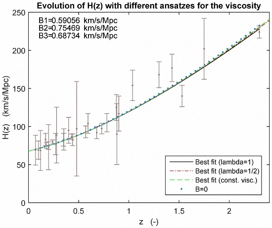
• A characteristic property as seen from the Figure 1 is that the differences between the predictions from the various viscosity models are relatively small. It may be surprising that even the simple ansatz $\zeta =$ constant reproduces experimental data quite well. These models however tend to underpredict $H\left(z\right)$ for large redshifts. In the literature, the ansatz $\zeta \propto \sqrt{\rho }$, is widely accepted.
• As for the magnitude of the bulk viscosity ${\zeta }_0$ in the present universe, we found, on the basis of various sources, that one hardly does better than restricting ${\zeta }_0$ to lie within an interval. We suggested the interval to extend from ${10}^4$ to ${10}^6$ Pa·s, although there are some indications that the upper limit could be extended somewhat. In any case, these are several orders of magnitude larger than the bulk viscosities encountered in usual hydrodynamics.
• In Section 5, we considered the future universe, extending from $t=0$ onwards. For definiteness, we chose the value ${\zeta }_0={10}^5$Pa·s. We focused on the occurrence of a big rip singularity in the far future. The numerical values found in the earlier sections enabled us to make a quantitative estimate of the rip time $t_s$. With α defined as $\alpha =w+1$, we found that even the case $\zeta ={\zeta }_0=$ constant allows the big rip to occur, if α is negative, i.e., lying in the phantom region. This is the same kind of behavior as found earlier by Caldwell [10] and others, in the non-viscous case. Of special interest is, however, the case $\zeta \propto \sqrt{\rho }$, where the fate of the universe is critically dependent on the magnitude of α. If $\alpha <0$, the big rip is inevitable, similarly as above. If $\alpha >0$ (the quintessence region), the big rip can actually also occur if α is very small, less than about 0.005. This possibility of sliding through the phantom divide was actually pointed out several years ago [8], but can now be better quantified. Typical rip times are found to lie roughly in the interval from 100 to 200 Gy.

References

1. Ade, P.A.R.; Aghanim, N.; Arnaud, M.; Ashdown, M.; Aumont, J.; Baccigalupi, C.; Banday, A.J.; Barreiro, R.B.; Bartlett, J.G.; Bartolo, N.; et al. Planck 2015 results. XIII. Cosmological parameters. 2015. [Google Scholar]
2. Nojiri, S.; Odintsov, S.D. Final state and thermodynamics of a dark energy universe. Phys. Rev. D 2004, 70. [Google Scholar] [CrossRef]
3. Nojiri, S.; Odintsov, S.D. Inhomogeneous equation of state of the universe: Phantom era, future singularity, and crossing the phantom barrier. Phys. Rev. D 2005, 72. [Google Scholar] [CrossRef]
4. Brevik, I. Viscosity-induced crossing of the phantom divide in the dark cosmic fluid. Front. Phys. 2013, 1, 27. [Google Scholar] [CrossRef] [Green Version]
5. Brevik, I. Crossing of the w = −1 barrier in viscous modified gravity. Int. J. Mod. Phys. D 2006, 15, 767–775. [Google Scholar] [CrossRef]
6. Brevik, I. Viscosity-induced crossing of the phantom barrier. Entropy 2015, 17, 6318–6328. [Google Scholar] [CrossRef] [Green Version]
7. Disconzi, M.M.; Kephart, T.W.; Scherrer, R.J. A new approach to cosmological bulk viscosity. Phys. Rev. D 2015, 91. [Google Scholar] [CrossRef]
8. Brevik, I.; Gorbunova, O. Dark energy and viscous cosmology. Gen. Relativ. Gravit. 2005, 37, 2039–2045. [Google Scholar] [CrossRef]
9. Stefancić, H. “Expansion” around the vacuum equation of state-sudden future singularities and asymptotic behavior. Phys. Rev. D 2005, 71, 118–120. [Google Scholar] [CrossRef]
10. Caldwell, R.R.; Kamionkowski, M.; Weinberg, N.N. Phantom energy: Dark energy with w less than −1 causes a cosmic doomsday. Phys. Rev. Lett. 2003, 91, 071301. [Google Scholar] [CrossRef] [PubMed]
11. Nojiri, S.; Odintsov, S.D. Quantum de Sitter cosmology and phantom matter. Phys. Lett. B 2003, 562, 147–152. [Google Scholar] [CrossRef]
12. Frampton, P.H.; Ludwick, K.J.; Scherrer, R.J. The little rip. Phys. Rev. D 2011, 84, 063003. [Google Scholar] [CrossRef]
13. Brevik, I.; Elizalde, E.; Nojiri, S.; Odintsov, S.D. Viscous little rip cosmology. Phys. Rev. D 2011, 84, 103508. [Google Scholar] [CrossRef]
14. Brevik, I.; Myrzakulov, R.; Nojiri, S.; Odintsov, S.D. Turbulence and little rip cosmology. Phys. Rev. D 2012, 86, 063007. [Google Scholar] [CrossRef]
15. Frampton, P.H.; Ludwick, K.J.; Scherrer, R.J. Pseudo-rip: Cosmological models intermediate between the cosmological constant and the little rip. Phys. Rev. D 2012, 85. [Google Scholar] [CrossRef]
16. Wei, H.; Wang, L.F.; Guo, X.J. Quasi-rip: A new type of rip model without cosmic doomsday. Phys. Rev. D 2012, 86, 1173–1188. [Google Scholar] [CrossRef]
17. Wang, J.; Meng, X. Effects of new viscosity model on cosmological evolution. Mod. Phys. Lett. A 2014, 29, 390–400. [Google Scholar] [CrossRef]
18. Velten, H.; Wang, J.; Meng, X. Phantom dark energy as an effect of bulk viscosity. Phys. Rev. D 2013, 88. [Google Scholar] [CrossRef]
19. Bamba, K.; Capozziello, S.; Nojiri, S.; Odintsov, S.D. Dark energy cosmology: The equivalent description via different theoretical models and cosmography tests. Astrophys. Space Sci. 2012, 342, 155–228. [Google Scholar] [CrossRef]
20. Elizalde, E.; Obukhov, V.V.; Timoshkin, A.V. Inhomogeneous viscous dark fluid coupled with dark matter in the FRW universe. Mod. Phys. Lett. A 2014, 29. [Google Scholar] [CrossRef]
21. Brevik, I.; Obukhov, V.V.; Timoshkin, A.V. Dark energy coupled with dark matter in viscous fluid cosmology. Astrophys. Space. Sci. 2015, 355, 399–403. [Google Scholar] [CrossRef]
22. Brevik, I.; Timoshkin, A.V. Viscous coupled fluids in inflationary cosmology. JETP 2016, 122, 679–684. [Google Scholar] [CrossRef]
23. Floerchinger, S.; Tetradis, N.; Wiedemann, U.A. Accelerating cosmological expansion from shear and bulk viscosity. Phys. Rev. Lett. 2015, 114, 091301. [Google Scholar] [CrossRef] [PubMed]
24. Brevik, I.; Gorbunova, O.; Nojiri, S.; Odintsov, S.D. On isotropic turbulence in the dark fluid universe. Eur. Phys. J. C 2011, 71, 1–7. [Google Scholar] [CrossRef]
25. Weinberg, S. Entropy generation and the survival of protogalaxies in an expanding universe. Astrophys. J. 1971, 68, 175. [Google Scholar] [CrossRef]
26. Weinberg, S. Gravitation and Cosmology; John Wiley & Sons: New York, NY, USA, 1972. [Google Scholar]
27. Zimdahl, W. ‘Understanding’ cosmological bulk viscosity. Mon. Not. R. Astron. Soc. 1996, 280, 1239–1243. [Google Scholar] [CrossRef]
28. Brevik, I.; Grøn, Ø. Relativistic Viscous Universe Models. In Recent Advances in Cosmology; Anderson, T., Brady, S., Eds.; Nova Scientific Publications: New York, NY, USA, 2013; pp. 99–127. [Google Scholar]
29. Bamba, K.; Odintsov, S.D. Inflation in a viscous fluid model. Eur. Phys. J. C 2016, 76, 1–12. [Google Scholar] [CrossRef]
30. Murphy, G.L. Big-bang model without singularities. Phys. Rev. D 1973, 8. [Google Scholar] [CrossRef]
31. Barrow, J.D. The deflationary universe: An instability of the de Sitter universe. Phys. Lett. B 1986, 180, 335–339. [Google Scholar] [CrossRef]
32. Li, W.J.; Ling, Y.; Wu, J.P.; Kuang, X.M. Thermal fluctuations in viscous cosmology. Phys. Lett. B 2010, 687, 1–5. [Google Scholar] [CrossRef]
33. Campo, S.D.; Herrera, R.; Pavon, D. Cosmological perturbations in warm inflationary models with viscous pressure. Phys. Rev. D. 2007, 75, 147–148. [Google Scholar]
34. Cardenas, V.H.; Cruz, N.; Villanueva, J.R. Testing a dissipative kinetic k-essence model. Eur. Phys. J. C 2015, 75. [Google Scholar] [CrossRef]
35. Nojiri, S.; Odintsov, S.D.; Tsujikawa, S. Properties of singularities in the (phantom) dark energy universe. Phys. Rev. D 2005, 71. [Google Scholar] [CrossRef]
36. De Paolis, F.; Jamil, M.; Quadir, A. Black holes in bulk viscous cosmology. Int. J. Theor. Phys. 2010, 49, 621–632. [Google Scholar] [CrossRef]
37. Van den Horn, L.J.; Salvati, G.A.Q. Cosmological two-fluid bulk viscosity. Mon. Not. R. Astron. Sci. 2016, 457, 1878–1887. [Google Scholar] [CrossRef]
38. Fay, S. Constraints from growth-rate data on some coupled dark energy models mimicking a ΛCDM expansion. 2016. [Google Scholar]
39. Chen, Y.; Geng, C.-Q.; Cao, S.; Huang, Y.-M.; Zhu, Z.-H. Constraints on a ϕCDM model from strong gravitational lensing and updated Hubble parameter measurements. J. Cosmol. Astropart. Phys. 2015, 2. [Google Scholar] [CrossRef]
40. Frampton, P.H. Cyclic Entropy: An alternative to inflationary cosmology. Int. J. Mod. Phys. A 2015, 30, 1550129. [Google Scholar] [CrossRef]
41. Velten, H.; Schwarz, D.J. Dissipation of dark matter. Phys. Rev. D 2012, 86, 083501. [Google Scholar] [CrossRef]
42. Brevik, I. Temperature variation in the dark cosmic fluid in the late universe. Mod. Phys. Lett. A 2016, 31. [Google Scholar] [CrossRef]
43. Sasidharan, A.; Mathew, T. Phase space analysis of bulk viscous matter dominated universe. 2015. [Google Scholar]
Figure 1. Friedmann’s first equation for H ( z ) (km·s - 1 Mpc - 1 ) with three different ansatzes for the viscosity. The fit-values used for B are (i) B 1 = 0.590 km·s - 1 Mpc - 1 for ζ ρ (solid, black line), (ii) B 2 = 0.755 km·s - 1 Mpc - 1 for ζ ρ (stippled, dotted red line) and (iii) B 3 = 0.687 km·s - 1 Mpc - 1 for constant viscosity (stippled, green line). The dotted blue line gives the corresponding evolution for B = 0 (no viscosity).
Entropy 18 00215 g001