Entropy and Stability Analysis of Delayed Energy Supply–Demand Model

Abstract

In this paper, a four-dimensional model of energy supply–demand with two-delay is built. The interactions among energy demand of east China, energy supply of west China and the utilization of renewable energy in east China are delayed in this model. We discuss stability of the system affected by parameters and the existence of Hopf bifurcation at the equilibrium point from two aspects: single delay and two-delay. The stability and complexity of the system are demonstrated through bifurcation diagram, Poincare section plot, entropy diagram, etc. in numerical simulation. The simulation results show that the parameters beyond the stable region will cause the system to be unstable and increase the complexity of the system. At this point, because of energy supply–demand system fluctuations, it is difficult to formulate energy policies. Finally, the bifurcation control is realized successfully by the method of delayed feedback control. The results of bifurcation control simulation indicate that the system can return to stable state by adjusting the control parameter. In addition, we find that the bigger the value of the control parameter, the better the effect of the bifurcation control. The results of this paper can provide help for maintaining the stability of the system, which will be conducive to energy scheduling.

1. Introduction

Energy is the foundation of the national economy. Because of the uneven distribution of natural resources and the difference of economic development in China, the energy demand in east China is relatively large. We generally take a variety of measures to meet the great demand for energy in east China, such as the energy transportation project from west to east, energy imports and the development of renewable energy. Many scholars have studied energy demand and supply and energy sustainable development. They have obtained many valuable results. Wu et al. [1] studied energy efficiency, environmental efficiency and the integration of energy and environmental measures. They obtained some valuable results. For instance, the energy-saving and emission-reduction efficiency in western and central China is worse than that in east China. Fang et al. [2] discussed the impact of carbon tax on energy intensity and economic growth in energy-saving and emission-reduction system. The dynamic characteristics of system are investigated on the basis of complexity theory and entropy theory. Liu et al. [3] put forward a lot of suggestions about layout optimization, structure adjustment and matching policy support. Their research results can provide theoretical reference and practical guidance for the sustainable development of China’s energy. Zhang et al. [4] took oil, coal, electricity and gas as the research object, and analyzed the energy supply–demand evolution process from 1997 to 2009. The results show that there is a huge difference in energy supply and energy demand in space. Their suggestions can promote the coordinated development of the region. Wang et al. [5] focused on the analysis of energy strategy, energy development and energy consumption of China. In addition, they also studied the Asia’s energy security project by the method of Long-range Energy Alternatives Planning, which played an important role in the future of energy and environmental policy. Zhang et al. [6] pointed out that China must implement energy-saving and emission-reduction to reduce environmental pollution and insist on sustainable development. Moreover, China must adhere to the development of renewable energy and clean energy, which is conducive to reducing the consumption of non-renewable energy sources.

Jiang et al. [7] put forward that China should develop low carbon economy and develop clean energy such as the renewable energy and new energy. Besides, China should increase publicity and legislation to promote national awareness of energy conservation and emission reduction, and protect the environment. Ma et al. [8] proposed a development strategy that can solve the energy demand of China. The research results show that China must improve the efficiency of energy-saving and emission-reduction, and give priority to the development of alternative energy sources. Li [9] studied the quantitative problem of sustainable energy strategy in China using the econometric method. Sun et al. [10] built a universal bipartite model based on an energy supply–demand network. They empirically analyzed the production’s SPL (Service Parts Logistics) distribution of the US coal companies from 1991 to 2009.

Sun et al. [11] the parameters of energy supply–demand system are determined through neural network method. They analyzed the dynamic behavior of the energy supply–demand system. The results show that the energy supply–demand system has the ability of self-regulation to ensure that the unstable system returns to a steady state. Hacatoglu et al. [12] an evaluation method for sustainable economic development by life-cycle emission factors and sustainability indicators is proposed. This method can ensure the sustainable and healthy development of the economy. Pereira et al. [13] discussed the development situation of the renewable energy market in Brazil and the theory of overcoming the obstacles of market development. The conclusions of this paper can provide help for the consolidation and development of renewable energy markets. Mulhall et al. [14] suggested that fluctuations in energy prices may affect the stability of individual firms and their supply chains. The extension of the time commitment of the energy supply contract entails the decrease can reduce the flexibility of the enterprise in the management of price changes. Toan et al. [15] studied the current status and trends of energy use in Vietnam, as well as the forecast of energy demand and supply in the coming decades. Buscarino et al. [16] investigated the problem of the design and the implementation of chaotic circuits with delay. The chaotic dynamic characteristics of the circuit are discussed.

A new four-dimensional energy supply–demand model was established in [17]. The model revealed the complex relationship of mutual support and mutual constraints among energy demand, energy imports and renewable energy utilization. The model in [17] is as follows:

$$\{\begin{array}{l}\frac{dx}{dt}=a_{1}x(1-\frac{x}{M})-a_{2}x(y+z)-d_{3}w,\\ \frac{dy}{dt}=-b_{1}y-b_{2}z+b_{3}x[N-(x-z)],\\ \frac{dz}{dt}=c_{1}z(c_{2}x-c_3),\\ \frac{dw}{dt}=d_{1}x-d_{2}w,\end{array}$$

(1)

where $x(t)$ is the energy demand in east China; $y(t)$ is energy supply in west China; $z(t)$ is the energy imports in east China; $w(t)$ is the utilization of renewable energy resources in east China; $a_1$ is the elasticity coefficient of energy consumption in east China; $a_2$ is the coefficient of the impact of energy supply in west China and energy imports on the energy demand in east China; $b_1$ is the influence coefficient of energy supply in west China on supply speed; $b_2$ is coefficient of the impact of energy imported in east China on the speed of energy supply; $b_3$ is the coefficient of the influence of energy demand in east China on the speed of energy supply; $c_1$ is speed of energy imported in east China; $c_2$ is income from unit energy imported; $c_3$ is the cost of energy imported; $d_1$ is the coefficient of the impact of energy demand in east China on the utilization of renewable energy; $d_2$ is the coefficient of the impact of the utilization of renewable energy in east China on the ratio of renewable energy utilization; $d_3$ is the coefficient of the influence of the utilization of renewable energy on energy demand in east China; M is the biggest energy demand in east China; N is the threshold of energy demand in east China; and $a_i,b_i,c_i,M,N>0,N<M$, which are all constant.

However, it takes time to develop and utilize renewable energy in east China. This paper considers only hydropower. China has an uneven distribution of hydropower resources. The available water resources in the eastern areas accounts only for 6% of the total amount of the nation while the southwestern areas have the lion share, taking up 67.8%. Meanwhile, the rainfall in east China tends to be the greatest in summer but waning in other seasons. We know that hydropower station needs to store water before they can generate electricity. Only when the water storage capacity exceeds the threshold, the hydropower station can complete the power output to meet the energy demand of economic development. We found that the power output lagged behind the storage capacity. In other words, meeting energy demand $x(t)$ also lagged behind the water storage capacity $w(t)$. We define this delay as ${\tau }_1$. There is a significant impact of rainfall on water storage capacity. With different seasons, ${\tau }_1$ changes significantly.

China has an uneven distribution of coal reserve: Xinjing, Inner Monglia, Shanxi and Shan’xi account for 81.3% of the total reserve while the eastern provinces 6%. However, the demand in the more developed eastern regions of China is much higher, as those 16 provinces and provincial cities in 2015 alone accounted for 67% of the nation’s GDP. The regional discrepancy in coal resources distribution and the gap in the demand and supply dictates the distinctive mode of “coal transporting from west to east”, which relies heavily on the coordinated transportation of railway and seaway in the coastal regions but is also supplemented with railway delivery, inland river and road transport.

In addition, since China is a large country geographically, it takes time for the energy sources in west China to be transported to east China. In this paper, we only consider coal transportation. That is to say, coal demand in east China $x(t)$ will lag behind the coal supply in west China $y(t)$. We define the delay as ${\tau }_2$. With the changes of coal mining in west China, conveyance and weather, ${\tau }_2$ changes obviously.

Therefore, on the basis of Model (1), we study the following model with two-delay:

$$\{\begin{array}{l}\frac{dx}{dt}=a_{1}x(1-\frac{x}{M})-a_{2}x(y(t-{\tau }_2)+z)-d_{3}w(t-{\tau }_1),\\ \frac{dy}{dt}=-b_{1}y-b_{2}z+b_{3}x[N-(x-z)],\\ \frac{dz}{dt}=c_{1}z(c_{2}x-c_3),\\ \frac{dw}{dt}=d_{1}x-d_{2}w,\end{array}$$

(2)

where the development speed of energy demand in east China $\frac{dx(t)}{dt}$ is proportional to the current demand for energy $x(t)$ and the development potential for energy demand $1-\frac{x(t)}{M}$; $-a_{2}y(t)$ stands for supply with energy from China’s western areas to the eastern ones, while $-a_{2}z(t)$ represents energy input by importing into China’s eastern areas reducing energy demand in east China; $-b_{1}y(t)$ stands for the curb against energy supply to China’s eastern areas from the western ones because of such factors as cost, ecological environment protection, etc.; $-b_{2}z(t)$ stands for reduction of energy supply from China’s western areas because of the imported energy input in China’s eastern areas; $b_{3}x(t)[N-x(t)-z(t)]$ indicates, when energy demand in China’s eastern areas is smaller than the threshold value $(x(t)-z(t)<N)$, the speed of energy supply of China’s eastern areas from China’s western areas increases as $x(t)$ increases; however, when energy demand in China’s eastern areas is big enough $(x(t)-z(t)>N)$, with the development of the regional economy in China’s west areas, Chinese western areas’ energy demand is greatly improved, energy supply velocity in the east will decrease as $x(t)$ increases; $c_{1}z(t)(c_{2}x(t)-c_3)$ shows that energy importing speed is restricted by energy demand in China’s eastern regions, as well as the cost of imported energy; $-d_{3}w$ indicates that the utility of renewable energy in eastern areas leads to decrease of the energy supply from China’s western regions; and $d_{1}x-d_{2}w$ symbolizes that the utility rate of renewable energy in China’s eastern areas $\frac{dw}{dt}$ increases as $x(t)$ rises and decreases as $w(t)$ goes up.

The rest of this paper is organized as follows. In Section 2, we build a four-dimensional energy supply–demand model with two-delay and study the local stability and the existence of Hopf bifurcation at the equilibrium point of Model (2). In Section 3, we discuss the impacts of parameters on the stability and entropy of Model (2). In Section 4, bifurcation control is achieved successfully using the method of delayed feedback control. Finally, conclusions are given in Section 5.

2. Local Stability and the Existence of Hopf Bifurcation

It is more difficult to get the equilibrium point directly in Model (2), so we assume that the equilibrium point of Model (2) is $E(x^{*},y^{*},z^{*},w^{*})$. We can obtain a specific equilibrium point of Model (2) with given parameters. In this paper, we will study the impacts of ${\tau }_1$,${\tau }_2$ and other parameters on the stability and entropy of Model (2) at the equilibrium point.

For simplicity, the linear form of Model (2) at the equilibrium point $E(x^{*},y^{*},z^{*},w^{*})$ through the Jacobian matrix is as follows [18]:

$$\{\begin{array}{l}\frac{dx}{dt}=(a_1-\frac{2a_1{x}^{*}}{M}-a_2{y}^{*}-a_2{z}^{*})x-a_2{x}^{*}y(t-{\tau }_2)-a_2{x}^{*}z-d_{3}w(t-{\tau }_1),\\ \frac{dy}{dt}=(b_{3}N-2b_3{x}^{*}+b_3{z}^{*})x-b_{1}y+(b_3{x}^{*}-b_2)z,\\ \frac{dz}{dt}=c_1{c}_2{z}^{*}x+(c_1{c}_2{x}^{*}-c_1{c}_3)z,\\ \frac{dw}{dt}=d_{1}x-d_{2}w,\end{array}$$

(3)

The determinant of Model (3) is:

$$\left|\begin{array}{cccc}\lambda -(a_1-\frac{2a_1{x}^{*}}{M}-a_2{y}^{*}-a_2{z}^{*})\hfill & a_2{x}^{*}{e}^{-\lambda {\tau }_2}& a_2{x}^{*}& d_3{e}^{-\lambda {\tau }_1}\\ -(b_{3}N-2b_3{x}^{*}+b_3{z}^{*})\hfill & \lambda +b_1& -(b_3{x}^{*}-b_2)& 0\\ -c_1{c}_2{z}^{*}\hfill & 0& \lambda -(c_1{c}_2{x}^{*}-c_1{c}_3)& 0\\ -d_1\hfill & 0& 0& \lambda +d_2\end{array}\right|=0$$

(4)

The characteristic equation of Model (3) is:

$${\lambda }^4+A_3{\lambda }^3+A_2{\lambda }^2+A_1\lambda +A_0+(B_2{\lambda }^2+B_1\lambda +B_0)e^{-\lambda {\tau }_1}+(C_2{\lambda }^2+C_1\lambda +C_0)e^{-\lambda {\tau }_2}=0$$

(5)

where

$$A_3=\frac{1}{M}2a_1{x}^{*}-a_1+b_1+d_2+c_1{c}_3+a_2{y}^{*}+a_2{z}^{*}-c_1{c}_2{x}^{*},$$

$$\begin{array}{ll}{A}_2=& -a_1{b}_1-a_1{d}_2+b_1{d}_2+\frac{1}{M}2a_1{b}_1{x}^{*}+\frac{1}{M}2a_1{d}_2{x}^{*}-\frac{1}{M}2a_1{c}_1{c}_2{x}^{*2}-a_1{c}_1{c}_3\\ & +b_1{c}_1{c}_3+c_1{c}_3{d}_2+a_2{b}_1{y}^{*}+a_2{b}_1{z}^{*}+a_2{d}_2{y}^{*}+a_2{d}_2{z}^{*}+\frac{1}{M}2a_1{c}_1{c}_3{x}^{*}\\ & +a_1{c}_1{c}_2{x}^{*}-b_1{c}_1{c}_2{x}^{*}+a_2{c}_1{c}_3{y}^{*}+a_2{c}_1{c}_3{z}^{*}-c_1{c}_2{d}_2{x}^{*}-a_2{c}_1{c}_2{x}^{*}{y}^{*}\end{array},$$

$$\begin{array}{ll}{A}_1=& -a_1{b}_1{d}_2+\frac{1}{M}2a_1{b}_1{d}_2{x}^{*}-\frac{1}{M}2a_1{b}_1{c}_1{c}_2{x}^{*}{}^2-\frac{1}{M}2a_1{c}_1{c}_2{d}_2{x}^{*}{}^2-a_1{b}_1{c}_1{c}_3-a_1{c}_1{c}_3{d}_2\\ & +b_1{c}_1{c}_3{d}_2+a_2{b}_1{d}_2{y}^{*}+a_2{b}_1{d}_2{z}^{*}+\frac{1}{M}2a_1{b}_1{c}_1{c}_3{x}^{*}+\frac{1}{M}2a_1{c}_1{c}_3{d}_2{x}^{*}+a_1{b}_1{c}_1{c}_2{x}^{*}\\ & +a_2{b}_1{c}_1{c}_3{y}^{*}+a_1{c}_1{c}_2{d}_2{x}^{*}+a_2{b}_1{c}_1{c}_3{z}^{*}-b_1{c}_1{c}_2{d}_2{x}^{*}+a_2{c}_1{c}_3{d}_2{y}^{*}+a_2{c}_1{c}_3{d}_2{z}^{*}\\ & -a_2{b}_1{c}_1{c}_2{x}^{*}{y}^{*}-a_2{c}_1{c}_2{d}_2{x}^{*}{y}^{*}\end{array},$$

$$\begin{array}{ll}{A}_0=& -\frac{1}{M}2a_1{b}_1{c}_1{c}_2{d}_2{x}^{*}{}^2-a_1{b}_1{c}_1{c}_3{d}_2+\frac{1}{M}2a_1{b}_1{c}_1{c}_3{d}_2{x}^{*}+a_1{b}_1{c}_1{c}_2{d}_2{x}^{*}\\ & +a_2{b}_1{c}_1{c}_3{d}_2{y}^{*}+a_2{b}_1{c}_1{c}_3{d}_2{z}^{*}-a_2{b}_1{c}_1{c}_2{d}_2{x}^{*}{y}^{*}\end{array},$$

$$B_2=d_1{d}_3,B_1=b_1{d}_1{d}_3+c_1{c}_3{d}_1{d}_3-c_1{c}_2{d}_1{d}_3{x}^{*},B_0=b_1{c}_1{c}_3{d}_1{d}_3-b_1{c}_1{c}_2{d}_1{d}_3{x}^{*},$$

$$C_2=-2a_2{b}_3{x}^{*}{}^2+N{a}_2{b}_3{x}^{*}+a_2{b}_3{x}^{*}{z}^{*},$$

$$\begin{array}{ll}{C}_1=& -2a_2{b}_3{d}_2{x}^{*}{}^2+N{a}_2{b}_3{d}_2{x}^{*}+a_2{b}_3{d}_2{x}^{*}{z}^{*}+2a_2{b}_3{c}_1{c}_2{x}^{*}{}^3-2a_2{b}_3{c}_1{c}_3{x}^{*}{}^2\\ & +N{a}_2{b}_3{c}_1{c}_3{x}^{*}-a_2{b}_2{c}_1{c}_2{x}^{*}{z}^{*}+a_2{b}_3{c}_1{c}_3{x}^{*}{z}^{*}-N{a}_2{b}_3{c}_1{c}_2{x}^{*}{}^2\end{array},$$

$$\begin{array}{ll}{C}_0=& 2a_2{b}_3{c}_1{c}_2{d}_2{x}^{*}{}^3-2a_2{b}_3{c}_1{c}_3{d}_2{x}^{*}{}^2+N{a}_2{b}_3{c}_1{c}_3{d}_2{x}^{*}\\ & -a_2{b}_2{c}_1{c}_2{d}_2{x}^{*}{z}^{*}+a_2{b}_3{c}_1{c}_3{d}_2{x}^{*}{z}^{*}-N{a}_2{b}_3{c}_1{c}_2{d}_2{x}^{*}{}^2\end{array}.$$

2.1. Case 1. ${\tau }_1>0,{\tau }_2=0$

When ${\tau }_1>0,{\tau }_2=0$, the characteristic equation of Model (3) becomes as below:

$${\lambda }^4+A_3{\lambda }^3+(A_2+C_2){\lambda }^2+(A_1+C_1)\lambda +A_0+C_0+(B_2{\lambda }^2+B_1\lambda +B_0)e^{-\lambda {\tau }_1}=0$$

(6)

Let $\lambda =i{\omega }_1({\omega }_1>0)$ be the root of Equation (6). Substituting $\lambda =i{\omega }_1({\omega }_1>0)$ into Equation (6) and separating the real and imaginary parts, we can get:

$$\{\begin{array}{l}(B_2{\omega }_1^2-B_0)\sin {\omega }_1{\tau }_1+B_1{\omega }_1\cos {\omega }_1{\tau }_1=A_3{\omega }_1^3+(A_1+C_1){\omega }_1\\ B_1{\omega }_1\sin {\omega }_1{\tau }_1-(B_2{\omega }_1^2-B_0)\cos {\omega }_1{\tau }_1=-{\omega }_1^4+(A_2+C_2){\omega }_1^2-(A_0+C_0)\end{array}$$

(7)

The following result can be obtained from Equation (7)

$$\cos {\omega }_1{\tau }_1=\frac{H_6{\omega }_1^6+H_4{\omega }_1^4+H_2{\omega }_1^2+H_0}{B_1^2{\omega }_1^2+{(B_2{\omega }_1^2-B_0)}^2}$$

(8)

where

$$H_6=B_2, H_4=A_3{B}_1-A_2{B}_2-B_2{C}_2+B_0,$$

$$H_2=A_1{B}_1+B_1{C}_1+A_0{B}_2+B_2{C}_0+A_2{B}_0+B_0{C}_2,H_0=-(A_0{B}_0+B_0{C}_0),$$

Adding up the squares of both equations given, we have

$${\omega }_1^8+h_6{\omega }_1^6+h_4{\omega }_1^4+h_2{\omega }_1^2+h_0=0$$

(9)

where

$$h_6=A_3^2-2A_2-2C_2,h_4=2A_1{A}_3+2A_3{C}_1+2A_0+2C_0-B_2^2+A_2^2+C_2^2+2A_2{C}_2,$$

$$h_2=A_1^2+C_1^2+2A_1{C}_1-2A_0{A}_2-2A_0{C}_2-2A_2{C}_0-2C_0{C}_2+2B_0{B}_2-B_1^2,$$

$$h_0={(A_0+C_0)}^2-B_0^2,$$

Let $s_1={\omega }_1^2$, Equation (9) is simplified as follows:

$$s_1^4+h_6{s}_1^3+h_4{s}_1^2+h_2{s}_1+h_0=0$$

(10)

According to Lemmas 2.1 and 2.2 in [19], we denote $h(s_1)=s_1^4+h_6{s}_1^3+h_4{s}_1^2+h_2{s}_1+h_0$. Thus, we can obtain that $(H_1)$: if $h_0<0$, Equation (10) has at least one positive root; $(H_2)$: if $h_0\ge 0$ and $D\ge 0$, Equation (10) has positive roots if and only if $s_{11}>0$ and $h\left(s_{11}\right)<0$; $(H_3)$: $h_0\ge 0$ and $D<0$, Equation (10) has positive roots if and only if there exists at least one $s_1^{*}\in \left\{s_{11},s_{12},s_{13}\right\}$, such that $s_1^{*}>0$ and $h(s_1^{*})<0$. Where

$$D={(\frac{q_1}{2})}^2+{(\frac{p_1}{3})}^3, p_1=\frac{h_4}{2}-\frac{3}{16}{h}_6^2, (H_2)q_1=\frac{h_6^3}{32}-\frac{h_6{h}_4}{8}+h_2, \sigma =\frac{-1+\sqrt{3}i}{2},$$

$$\begin{gathered} y_1=\sqrt[3]{-\frac{q_1}{2}+\sqrt{D}}+\sqrt[3]{-\frac{q_1}{2}-\sqrt{D}}, y_2=\sqrt[3]{-\frac{q_1}{2}+\sqrt{D}}\sigma +\sqrt[3]{-\frac{q_1}{2}-\sqrt{D}}{\sigma }^2, \\ {y}_3=\sqrt[3]{-\frac{q_1}{2}+\sqrt{D}}{\sigma }^2+\sqrt[3]{-\frac{q_1}{2}-\sqrt{D}}\sigma , s_{1i}=y_i-\frac{3h_6}{4}, i=1,2,3 \end{gathered}$$

Suppose that Equation (10) has positive roots. Without loss of generality, we suppose that it has four positive roots, defined by $s_{1k}$, $k=1,2,3,4$. Then, Equation (9) also has four positive roots; that is, ${\omega }_{1k}=\sqrt{s_{1k}}$, $k=1,2,3,4$. For every fixed ${\omega }_{1k}(k=1,2,3,4)$, there exists a sequence $\left\{{\tau }_{1k}^{(j)}|k=1,2,3,4;j=0,1,2,\mathrm{...}\right\}$. From Equation (8), we have:

$$\begin{array}{l}{\tau }_{1k}^{(j)}=\frac{1}{w_{1k}}\arccos \frac{H_6{\omega }_{1k}^6+H_4{\omega }_{1k}^4+H_2{\omega }_{1k}^2+H_0}{B_1^2{\omega }_{1k}^2+{(B_2{\omega }_{1k}^2-B_0)}^2}+\frac{2j\pi }{{\omega }_{1k}}\\ k=1,2,3,4;j=0,1,2,\mathrm{...}\end{array}$$

(11)

Let ${\tau }_{10}=\min \left\{{\tau }_{1k}^{(j)}\right|k=1,2,3,4;j=0,1,2,\mathrm{...}\}=\min \{{\tau }_{1k}^{(0)}|k=1,2,3,4\}={\tau }_{1k_0}$, then ${\omega }_{10}={\omega }_{1k_0}$.Thus, we get ${\tau }_{10}$ as follows:

$${\tau }_{10}=\frac{1}{w_{10}}\arccos \frac{H_6{\omega }_{10}^6+H_4{\omega }_{10}^4+H_2{\omega }_{10}^2+H_0}{B_1^2{\omega }_{10}^2+{(B_2{\omega }_{10}^2-B_0)}^2}$$

(12)

Based on the analysis above, we can obtain the following main results [20]:

Lemma 1.

If conditions $(H_1)-(H_3)$ have at least one hold, Equation (6) has a pair of purely imaginary roots $\pm i{\omega }_{10}$ when ${\tau }_1={\tau }_{10}$.

Next, take the derivative with ${\tau }_1$ in Equation (6), we have:

$${\left[\frac{d\lambda }{d{\tau }_1}\right]}^{-1}=\frac{(4{\lambda }^3+3A_3{\lambda }^2+2(A_2+C_2)\lambda +A_1+C_1)e^{\lambda {\tau }_1}+2B_2\lambda +B_1}{\lambda (B_2{\lambda }^2+B_1\lambda +B_0)}-\frac{{\tau }_1}{\lambda }$$

(13)

$${\left[\frac{d\lambda ({\tau }_{10})}{d{\tau }_1}\right]}_{\lambda =i{\omega }_{10}}^{-1}=\frac{R_1{R}_2+I_1{I}_2}{R_1^2+I_1^2}$$

(14)

where

$$R_1=-B_1{\omega }_{10}^2, I_1=B_0{\omega }_{10}-B_2{\omega }_{10}^3,$$

$$R_2=4{\omega }_{10}^3\sin {\omega }_{10}{\tau }_{10}-3A_3{\omega }_{10}^2\cos {\omega }_{10}{\tau }_{10}-2(A_2+C_2){\omega }_{10}\sin {\omega }_{10}{\tau }_{10}+(A_1+C_1)\cos {\omega }_{10}{\tau }_{10}+B_{10},$$

$$I_2=-4{\omega }_{10}^3\cos {\omega }_{10}{\tau }_{10}-3A_3{\omega }_{10}^2\sin {\omega }_{10}{\tau }_{10}+2(A_2+C_2){\omega }_{10}\cos {\omega }_{10}{\tau }_{10}+(A_1+C_1)\sin {\omega }_{10}{\tau }_{10}+2B_2{\omega }_{10}.$$

Lemma 2.

If $R_1{R}_2+I_1{I}_2\ne 0$, then ${\frac{d\mathrm{Re}\lambda ({\tau }_{10})}{d{\tau }_1}|}_{\lambda =i{\omega }_{10}}=\mathrm{Re}{\left[\frac{d\lambda ({\tau }_{10})}{d{\tau }_1}\right]}_{\lambda =i{\omega }_{10}}^{-1}\ne 0$. Thus, it satisfies the transversal condition.

According to Lemmas 1 and 2 and the Hopf bifurcation theorem in [21], we obtain the following results:

Theorem 1.

The equilibrium point $E(x^{*},y^{*},z^{*},u^{*})$ of Model (2) is asymptotically stable for ${\tau }_1\in [0,{\tau }_{10})$ and unstable for ${\tau }_1>{\tau }_{10}$. Model (2) has a Hopf bifurcation when ${\tau }_1={\tau }_{10}$.

2.2. Case 2. ${\tau }_1>0,{\tau }_2>0$

When ${\tau }_1>0,{\tau }_2>0$, the characteristic equation of Model (2) is still Equation (5). In this case, we consider the characteristic Equation (5) with ${\tau }_1$ in its stable intervals, i.e., ${\tau }_1\in [0,{\tau }_{10})$ [22]. We study the impact of ${\tau }_2$ on the stability of Model (2) when ${\tau }_1$ unchanged.

Let $\lambda =i{\omega }_2({\omega }_2>0)$ be a root of Equation (5). Similar to case1, we have:

$$\{\begin{array}{l}(C_2{\omega }_2^2-C_0)\sin {\omega }_2{\tau }_2+C_1{\omega }_2\cos {\omega }_2{\tau }_2=A_3{\omega }_2^3-A_1{\omega }_2-B_2{\omega }_2^2\sin {\omega }_2{\tau }_1-B_1{\omega }_2\cos {\omega }_2{\tau }_1+B_0\sin {\omega }_2{\tau }_1\\ C_1{\omega }_2\sin {\omega }_2{\tau }_2-(C_2{\omega }_2^2-C_0)\cos {\omega }_2{\tau }_2=-{\omega }_2^4+A_2{\omega }_2^2-A_0+B_2{\omega }_2^2\cos {\omega }_2{\tau }_1-B_1{\omega }_2\sin {\omega }_2{\tau }_1-B_0\cos {\omega }_2{\tau }_1\end{array}$$

(15)

From Equation (15), we obtain:

$$\cos {\omega }_2{\tau }_2=\frac{\Delta }{C_1^2{\omega }_2^2+{(C_2{\omega }_2^2-C_0)}^2}$$

(16)

where

$$\begin{array}{ll}\Delta =& A_3{C}_1{\omega }_2^3-A_1{C}_1{\omega }_2-B_2{C}_1{\omega }_2^2\sin {\omega }_2{\tau }_1-B_1{C}_1{\omega }_2\cos {\omega }_2{\tau }_1+B_0{C}_1\sin {\omega }_2{\tau }_1+C_2{\omega }_2^6\\ & -A_2{C}_2{\omega }_2^4+A_0{C}_2{\omega }_2^2-B_2{C}_2{\omega }_2^4\cos {\omega }_2{\tau }_1+B_1{C}_2{\omega }_2^3\sin {\omega }_2{\tau }_1+B_0{C}_2{\omega }_2^2\cos {\omega }_2{\tau }_1-C_0{\omega }_2^4\\ & +A_2{C}_0{\omega }_2^2-A_0{C}_0+B_2{C}_0{\omega }_2^2\cos {\omega }_2{\tau }_1-B_1{C}_0{\omega }_2\sin {\omega }_2{\tau }_1-B_0{C}_0\cos {\omega }_2{\tau }_1\end{array},$$

From Equation (15), we further get:

$${\omega }_2^8+n_7{\omega }_2^7+n_6{\omega }_2^6+n_5{\omega }_2^5+n_4{\omega }_2^4+n_3{\omega }_2^3+n_2{\omega }_2^2+n_1{\omega }_2+n_0=0$$

(17)

where

$$n_7=0, n_6=A_3^2-2A_2-2B_2\cos {\omega }_2{\tau }_1, n_5=-2A_3{B}_2\sin {\omega }_2{\tau }_1+2B_1\sin {\omega }_2{\tau }_1,$$

$$n_4=-2A_1{A}_3-C_2^2+B_2^2-2A_3{B}_1\cos {\omega }_2{\tau }_1+A_2^2+2A_0+2A_2{B}_2\cos {\omega }_2{\tau }_1+2B_0\cos {\omega }_2{\tau }_1,$$

$$n_3=2A_1{B}_2\sin {\omega }_2{\tau }_1+2A_3{B}_0\sin {\omega }_2{\tau }_1-2A_2{B}_1\sin {\omega }_2{\tau }_1,$$

$$n_2=A_1^2-C_1^2+2C_0{C}_2+2A_1{B}_1\cos {\omega }_2{\tau }_1-2B_0{B}_2-2A_0{A}_2-2A_0{B}_2\cos {\omega }_2{\tau }_1+B_1^2-2A_2{B}_0\cos {\omega }_2{\tau }_1,$$

$$n_1=2A_0{B}_1\sin {\omega }_2{\tau }_1-2A_1{B}_0\sin {\omega }_2{\tau }_1, n_0=B_0^2+A_0^2+2A_0{B}_0\cos {\omega }_2{\tau }_1-C_0^2,$$

Denote

$$h({\omega }_2)={\omega }_2^8+n_7{\omega }_2^7+n_6{\omega }_2^6+n_5{\omega }_2^5+n_4{\omega }_2^4+n_3{\omega }_2^3+n_2{\omega }_2^2+n_1{\omega }_2+n_0$$

Because $\underset{{\omega }_2\to \infty }{\lim }h({\omega }_2)=\infty$, we conclude that if $n_0<0$, then Equation (17) has at least one positive root [19]. Without loss of generality, we assume that Equation (17) has a finite number of positive roots defined by ${\omega }_{21},{\omega }_{22},{\omega }_{23},\mathrm{...},{\omega }_{2k}$, respectively. Fix each ${\omega }_{2i}$, $(i=1,2,\mathrm{...},k)$, and there is a series $\left\{{\tau }_{2i}^{(j)}|i=1,2,\mathrm{...},k;j=0,1,2,\mathrm{...}\right\}$ which satisfies Equation (17). From Equation (16), we can obtain:

$${\tau }_{2i}^{(j)}=\frac{1}{{\omega }_{2i}}\arccos \frac{\Delta }{C_1^2{\omega }_{2i}^2+{(C_2{\omega }_{2i}^2-C_0)}^2}+\frac{2j\pi }{{\omega }_{2i}},i=1,2,\mathrm{...},k;j=0,1,2,\mathrm{...}$$

(18)

Let ${\tau }_{20}=\min \{{\tau }_{2i}^{(j)}|i=1,2,\mathrm{...},k;j=0,1,2,\mathrm{...}\}=\underset{i\in \{1,2,\mathrm{...},k\}}{min}\{{\tau }_{2i}^{(0)}\}={\tau }_{2i_0}$, ${\omega }_{20}={\omega }_{2i_0}$. Then ${\tau }_{20}$ is:

$${\tau }_{20}=\frac{1}{{\omega }_{20}}\arccos \frac{{\Delta }^{\prime }}{C_1^2{\omega }_{20}^2+{(C_2{\omega }_{20}^2-C_0)}^2}$$

(19)

$$\begin{array}{ll}{\Delta }^{\prime }=& A_3{C}_1{\omega }_{20}^3-A_1{C}_1{\omega }_{20}-B_2{C}_1{\omega }_{20}^2\sin {\omega }_{20}{\tau }_1-B_1{C}_1{\omega }_{20}\cos {\omega }_{20}{\tau }_1+B_0{C}_1\sin {\omega }_{20}{\tau }_1+C_2{\omega }_{20}^6\\ & -A_2{C}_2{\omega }_{20}^4+A_0{C}_2{\omega }_{20}^2-B_2{C}_2{\omega }_{20}^4\cos {\omega }_{20}{\tau }_1+B_1{C}_2{\omega }_{20}^3\sin {\omega }_{20}{\tau }_1+B_0{C}_2{\omega }_{20}^2\cos {\omega }_{20}{\tau }_1-C_0{\omega }_{20}^4\\ & +A_2{C}_0{\omega }_{20}^2-A_0{C}_0+B_2{C}_0{\omega }_{20}^2\cos {\omega }_{20}{\tau }_1-B_1{C}_0{\omega }_{20}\sin {\omega }_{20}{\tau }_1-B_0{C}_0\cos {\omega }_{20}{\tau }_1\end{array}.$$

In the basis of the above analysis, we can obtain the following conclusion:

Lemma 3.

If $n_0<0$, the $\pm i{\omega }_{20}$ is a pair of purely imaginary roots of Equation (5) when ${\tau }_2={\tau }_{20}$ and ${\tau }_1\in [0,{\tau }_{10})$.

Next, we take the derivative of $\lambda$ with respect to ${\tau }_2$ in Equation (5), we can obtain:

$${\left[\frac{d\lambda }{d{\tau }_2}\right]}^{-1}=\frac{N_4+N_3+N_2+N_1}{N_0}-\frac{{\tau }_2}{\lambda }$$

(20)

where

$$N_4=(4{\lambda }^3+3A_3{\lambda }^2+2A_2\lambda +A_1)e^{\lambda {\tau }_2}, N_3=(2B_2\lambda +B_1)e^{\lambda ({\tau }_2-{\tau }_1)},$$

$$N_2=-{\tau }_1(B_2{\lambda }^2+B_1\lambda +B_0)e^{\lambda ({\tau }_2-{\tau }_1)}, N_1=2C_2\lambda +C_1,N_0=\lambda (C_2{\lambda }^2+C_1\lambda +C_0),$$

Taking $\lambda =i{\omega }_{20} ({\omega }_{20}>0)$ into Equation (20), we get:

$${\left[\frac{d\lambda ({\tau }_{20})}{d{\tau }_2}\right]}_{\lambda =i{\omega }_{20}}^{-1}=\frac{R_3{R}_4+I_3{I}_4}{R_3^2+I_3^2}$$

(21)

where

$$R_3=-C_1{\omega }_{20}^2, I_3=C_0{\omega }_{20}-C_2{\omega }_{20}^3,$$

$$\begin{array}{ll}{R}_4& =4{\omega }_{20}^3\sin {\omega }_{20}{\tau }_{20}-3A_3{\omega }_{20}^2\cos {\omega }_{20}{\tau }_{20}-2A_2{\omega }_{20}\sin {\omega }_{20}{\tau }_{20}+A_1\cos {\omega }_{20}{\tau }_{20}-2B_2{\omega }_{20}\sin {\omega }_{20}({\tau }_{20}-{\tau }_1)\\ & +B_1\cos {\omega }_{20}({\tau }_{20}-{\tau }_1)+B_2{\tau }_1{\omega }_{20}^2\cos {\omega }_{20}({\tau }_{20}-{\tau }_1)+B_1{\tau }_1{\omega }_{20}\sin {\omega }_{20}({\tau }_{20}-{\tau }_1)-B_0{\tau }_1\cos {\omega }_{20}({\tau }_{20}-{\tau }_1)+C_1\end{array},$$

$$\begin{array}{ll}{I}_4=& -4{\omega }_{20}^3\cos {\omega }_{20}{\tau }_{20}-3A_3{\omega }_{20}^2\sin {\omega }_{20}{\tau }_{20}+2A_2{\omega }_{20}\cos {\omega }_{20}{\tau }_{20}+A_1\sin {\omega }_{20}{\tau }_{20}+2B_2{\omega }_{20}\cos {\omega }_{20}({\tau }_{20}-{\tau }_1)\\ & +B_1\sin {\omega }_{20}({\tau }_{20}-{\tau }_1)+B_2{\tau }_1{\omega }_{20}^2\sin {\omega }_{20}({\tau }_{20}-{\tau }_1)-B_1{\tau }_1{\omega }_{20}\cos {\omega }_{20}({\tau }_{20}-{\tau }_1)-B_0{\tau }_1\sin {\omega }_{20}({\tau }_{20}-{\tau }_1)+2C_2{\omega }_{20}\end{array},$$

Owing to

$$sign\left[\frac{d(\mathrm{Re}\lambda ({\tau }_{20}))}{d{\tau }_2}\right]=sign\mathrm{Re}{\left[\frac{d\lambda ({\tau }_{20})}{d{\tau }_2}\right]}^{-1}$$

Lemma 4.

If $R_3{R}_4+I_3{I}_4\ne 0$, then ${\left[\frac{d\lambda ({\tau }_{20})}{d{\tau }_2}\right]}_{\lambda =i{\omega }_{20}}^{-1}\ne 0$. Therefore, Model (2) satisfies the transversal condition.

On the basis of Lemmas 3 and 4 and the Hopf bifurcation theorem in [21], we obtain the following results:

Theorem 2.

For ${\tau }_1\in [0,{\tau }_{10})$, ${\tau }_{10}$ is defined by Equation (12). The equilibrium point $E(x^{*},y^{*},z^{*},u^{*})$ of Model (2) is asymptotically stable for ${\tau }_2\in [0,{\tau }_{20})$ and unstable when ${\tau }_2>{\tau }_{20}$. Model (2) undergoes a Hopf bifurcation at ${\tau }_2={\tau }_{20}$.

3. Numerical Simulation and Analysis

In this section, we verify the correctness of the theoretical analysis and discuss the effect of the parameters on the stability of the system by numerical simulation. Let $a_1=1$; $a_2=0.6$; $b_1=1$; $b_2=1.2$; $b_3=1.5$; $c_1=11$; $c_2=0.7;$ $c_3=0.6$; $M=3.8$; $N=1.2$; $d_1=0.1$; $d_2=0.7$; $d_3=0.8$; $x(0)=1$; $y(0)=0.8$; $z(0)=0.6$; $w(0)=0.4$. Thus, we consider the following model:

$$\{\begin{array}{l}\frac{dx}{dt}=x(1-\frac{x}{3.8})-0.6x(y(t-{\tau }_2)+z)-0.8w(t-{\tau }_1),\\ \frac{dy}{dt}=-y-1.2z+1.5x[1.2-(x-z)],\\ \frac{dz}{dt}=11z(0.7x-0.6),\\ \frac{dw}{dt}=0.1x-0.7w,\end{array}$$

(22)

It is easy to get the equilibrium point of Model (22). However, only $E(0.8572,0.4929,0.6088,0.1225)$ conforms to the economic significance. It means that $x(t)$, $y(t)$, $z(t)$ and $u(t)$ will converge to the equilibrium point $E$ through the game.

For case 1, when ${\tau }_1>0,{\tau }_2=0$, we get ${\tau }_{10}=0.2208$,${\omega }_{10}=3.5247$ by Equations (10) and (12). In addition, we can obtain $R_1{R}_2+I_1{I}_2=86.8936\ne 0$, $h_0=-36.4229<0$. According to Theorem 1, we obtain that the equilibrium point $E$ of Model (22) is asymptotically stable when ${\tau }_1\in [0,0.2208)$ and unstable when ${\tau }_1>0.2208$. It has a Hopf bifurcation at ${\tau }_1=0.2208$.

For case 2, when ${\tau }_1>0,\tau >0$, let ${\tau }_1=0.1\in [0,0.2208)$, we can obtain ${\tau }_{20}=0.1429$, ${\omega }_{20}=5.4496$ through Equations (17) and (19). Besides, we get $R_3{R}_4+I_3{I}_4=67.3428\ne 0$, $n_0=-47.6814<0$. According to Theorem 2, we can obtain that the equilibrium point $E$ of Model (22) is asymptotically stable when ${\tau }_2\in [0,0.1429)$ for ${\tau }_1=0.1$ and unstable when ${\tau }_2>0.1429$ for ${\tau }_1=0.1$. It undergoes a Hopf bifurcation when ${\tau }_2=0.1429$ for ${\tau }_1=0.1$.

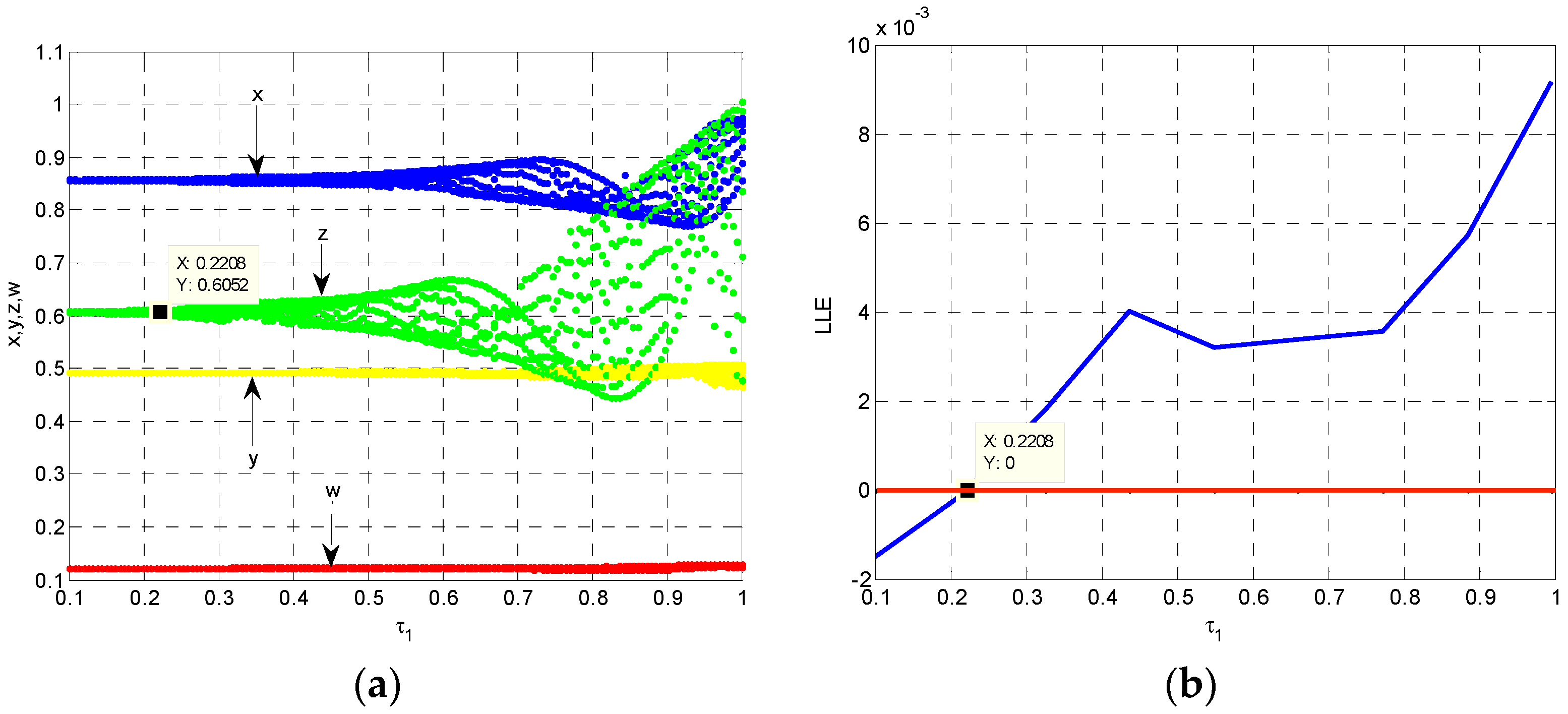
3.1. The Influence of ${\tau }_1$ on the Stability of Equation (22)

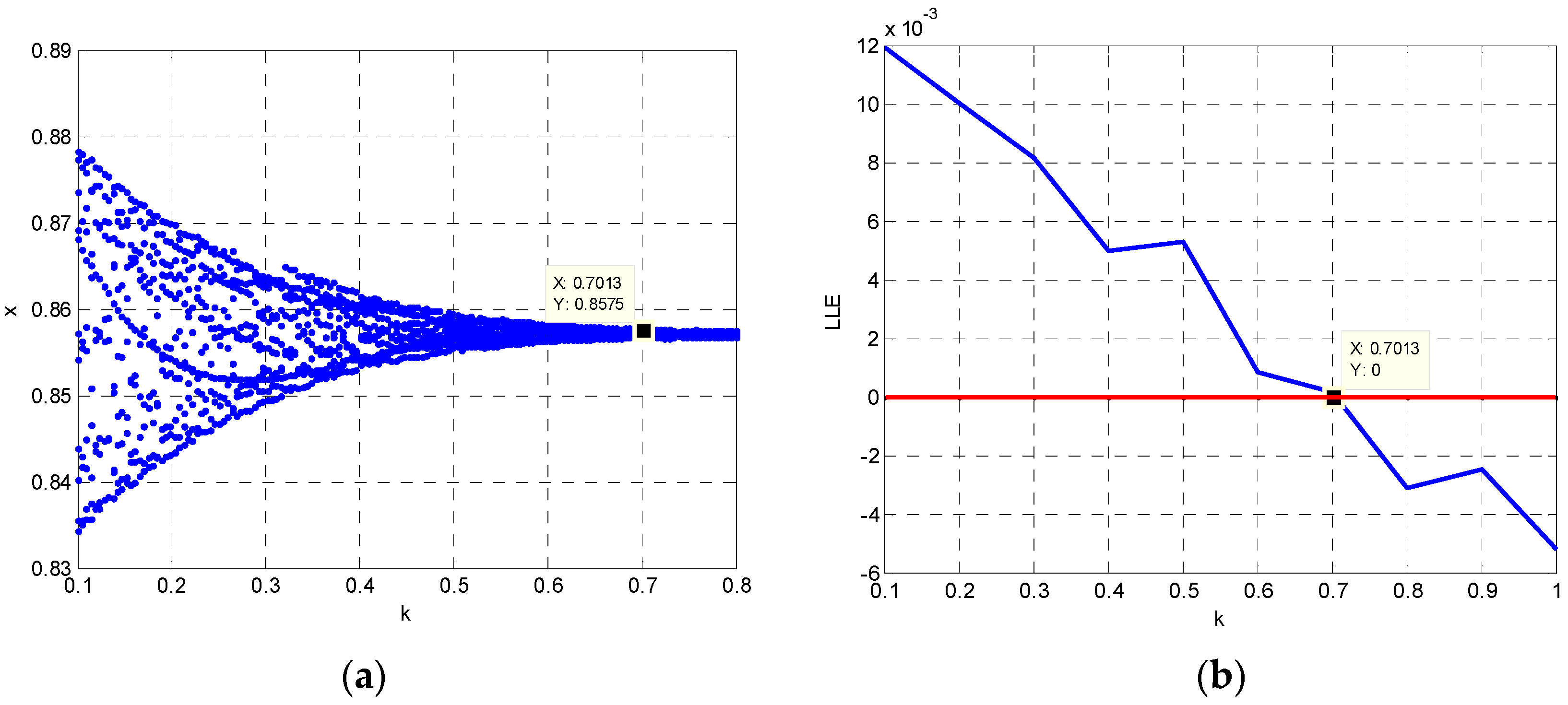
Model (22) shifts from stable to unstable with the increase of ${\tau }_1$, and it has a Hopf bifurcation at ${\tau }_1=0.2208$ when ${\tau }_2=0$. Figure 1a shows the dynamic evolution process of Model (22). We can see clearly that energy demand $x(t)$ and energy imports $z(t)$ in east China show an obvious bifurcation. The largest Lyapunov exponent (LLE) judges whether the system is stable depending on the exponent value. If it is less than 0, the system is stable. If it is more than 0, the system is unstable. If it is equal to 0, the system appears bifurcation. In this paper, we calculate the LLE by using the method of Wolf reconstruction [23]. We find that the value of the LLE is equal to 0 when ${\tau }_1=0.2208$ in Figure 1b. That is to say, Model (22) appears bifurcation at ${\tau }_1=0.2208$. This is consistent with the conclusion of theoretical analysis. Figure 1b also verifies the correctness of evolution process in Figure 1a.

Figure 1. The impact of ${\tau }_1$ on the stability of Model (22) when ${\tau }_2=0$: (a) bifurcation diagram; and (b) the largest Lyapunov exponent plot.

According to the above analysis, we can conclude that if time interval between storage of water and power output in hydroelectric power is greater than the bifurcation value in Model (22), it will cause the energy demand $x(t)$ and energy imports $z(t)$ to be unstable and fluctuant. The unstable energy supply–demand system is not conducive to the determination of energy demand and energy allocation.

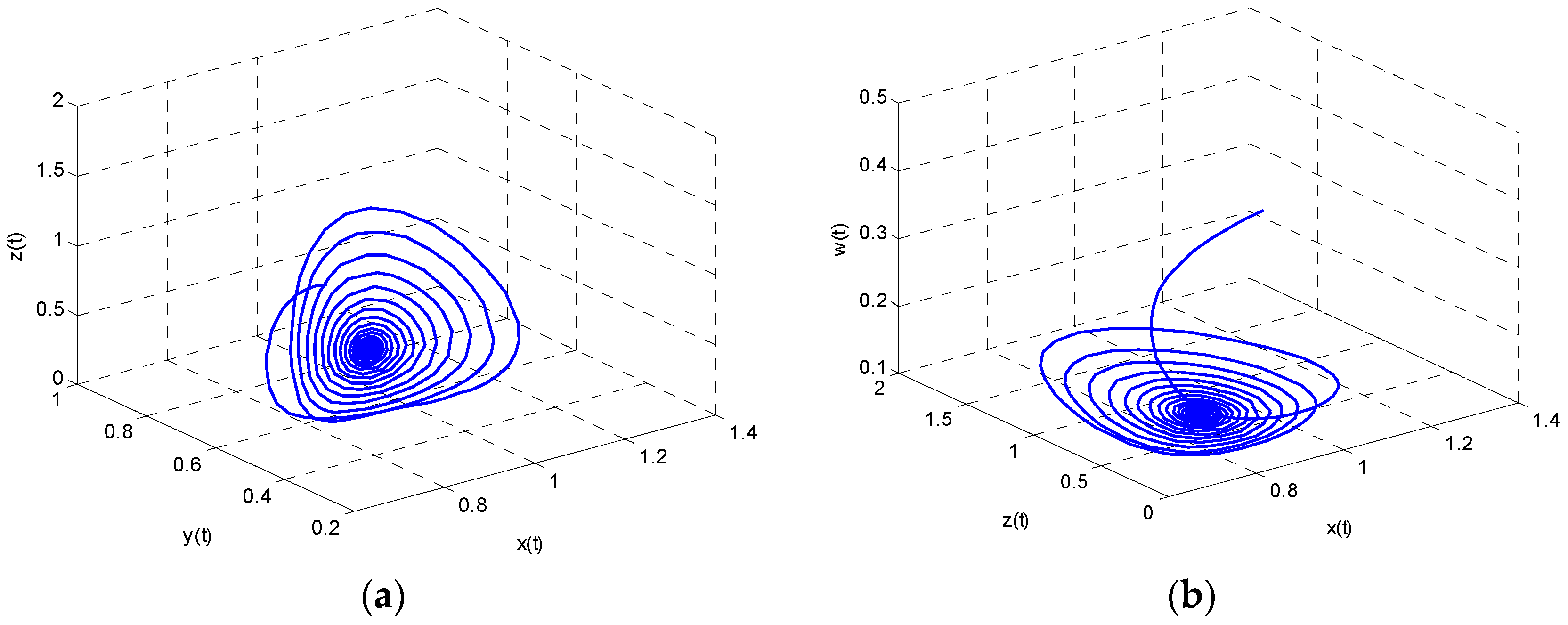
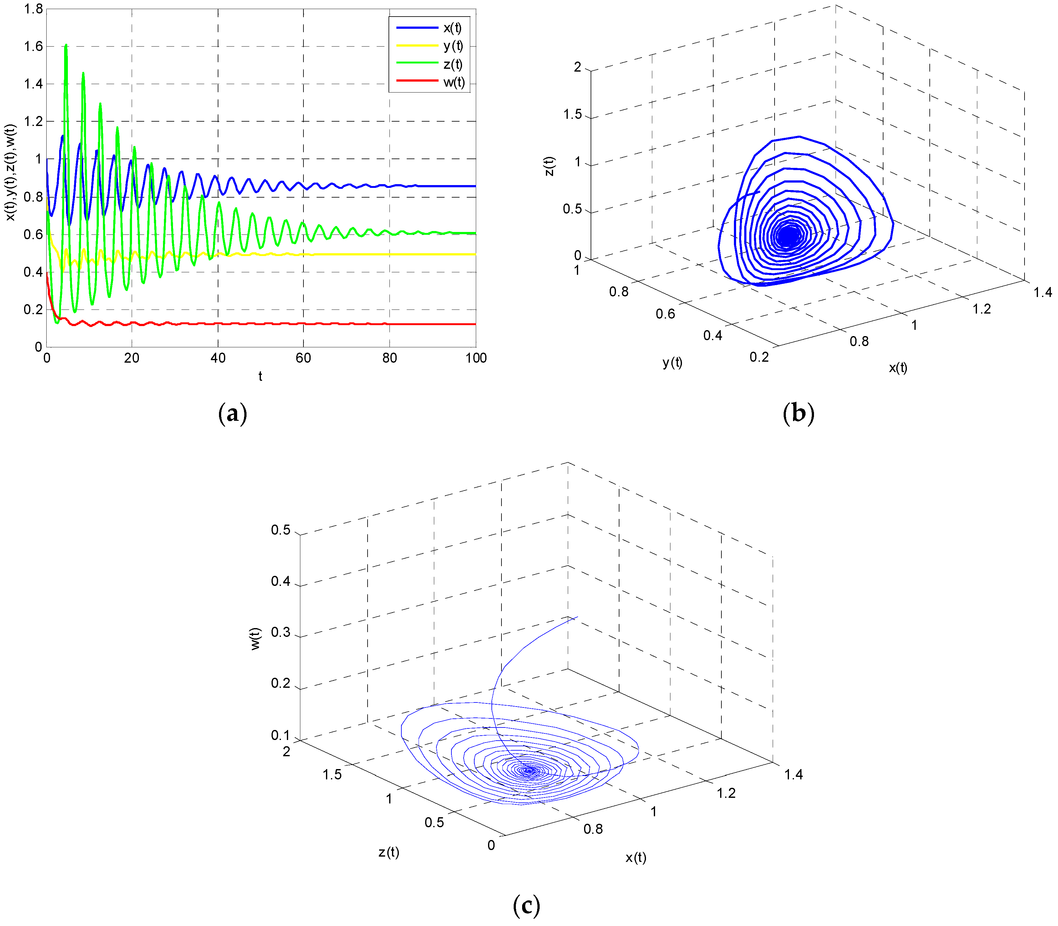
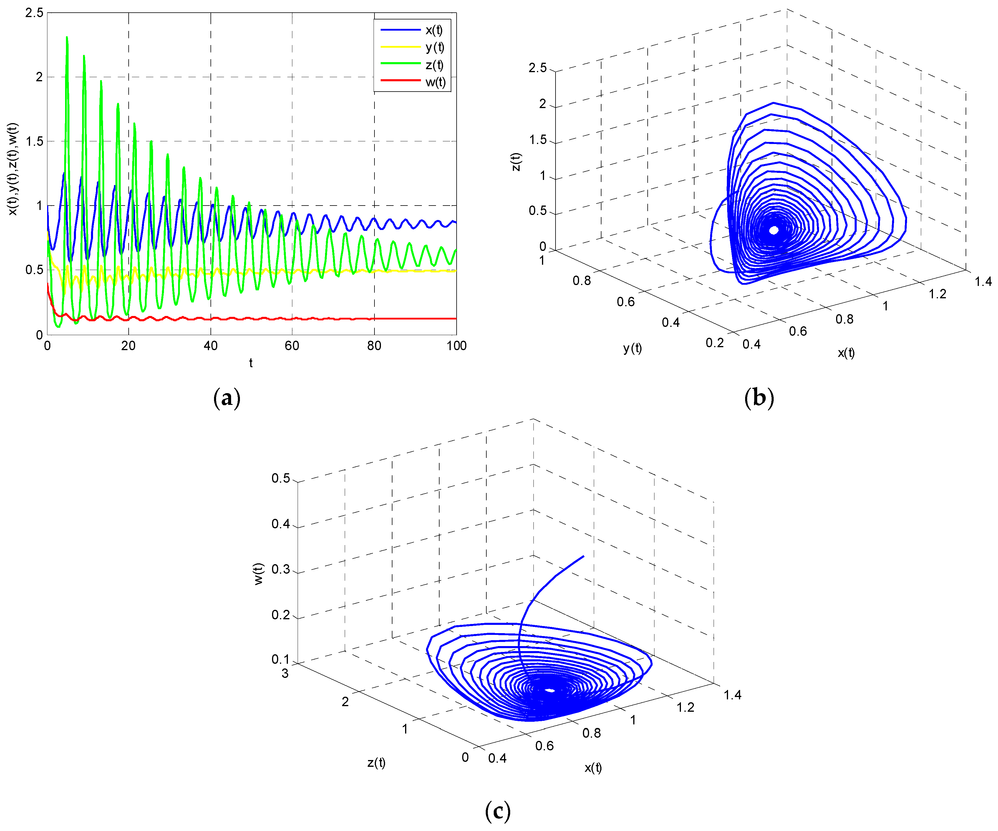
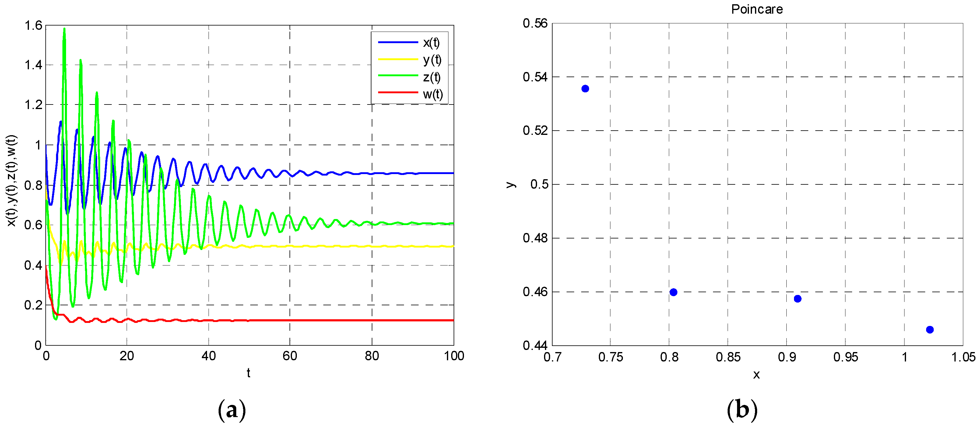
According to Theorem 1, Model (22) is stable when ${\tau }_1=0.1<{\tau }_{10}=0.2208,{\tau }_2=0$. These properties are shown in Figure 2 and Figure 3. As the time variable increases, Model (22) tends to be stable as is shown in Figure 2a, which means that the energy supply–demand system has self-repair ability to return to a steady state when ${\tau }_1<{\tau }_{10},{\tau }_2=0$. Moreover, Poincare section is an effective tool to judge the state of the system. There are four discrete points in Figure 2b, which shows that the system is stable.

Figure 2. (a) Time-domain plot; and (b) Poincare section when ${\tau }_1=0.1<{\tau }_{10}=0.2208$, ${\tau }_2=0$.

Figure 3. The attractor of Model (22) when ${\tau }_1=0.1<{\tau }_{10}=0.2208$, ${\tau }_2=0$: (a) $x(t),y(t),z(t)$; and (b) $x(t),z(t),w(t)$.

Attractor indicates the final state of the system runs. It can be seen that the system tends to equilibrium point $E(0.8572,0.4929,0.6088,0.1225)$ finally. That means each participant in the energy supply–demand system has obtained the best strategy through the game and that the whole system is in a stable state. It will contribute to the formulation of energy supply and demand policy. Figure 3 shows the dynamic evolution of the attractor.

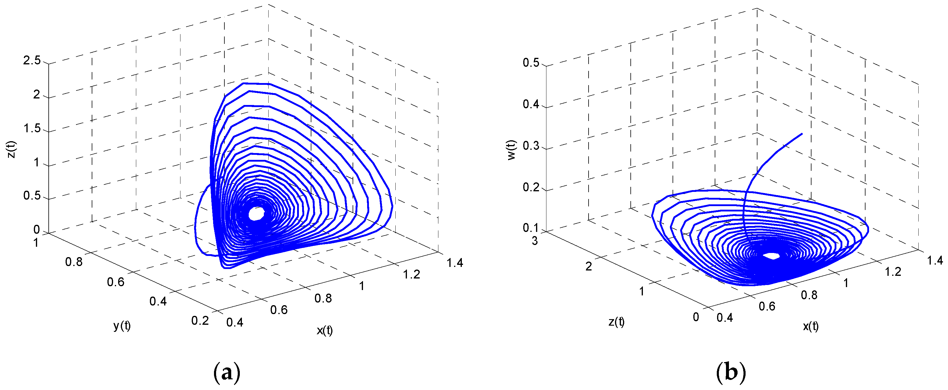
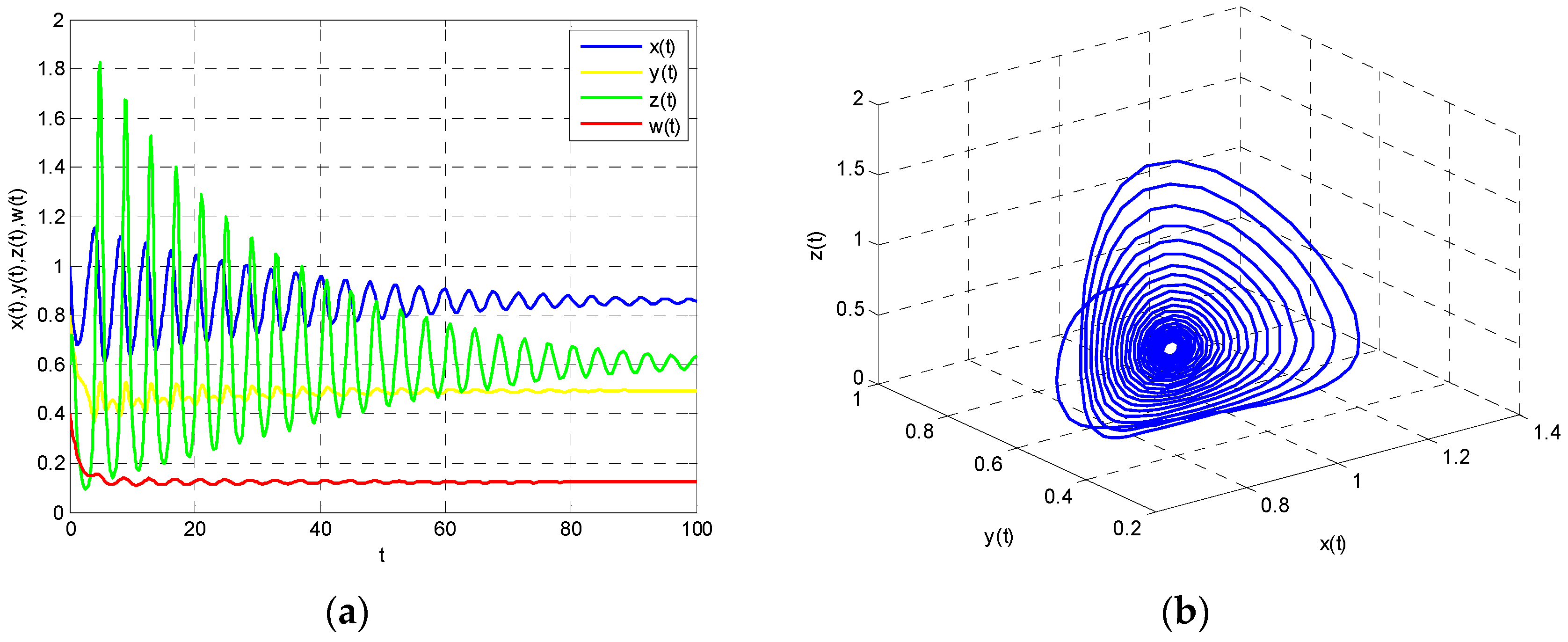
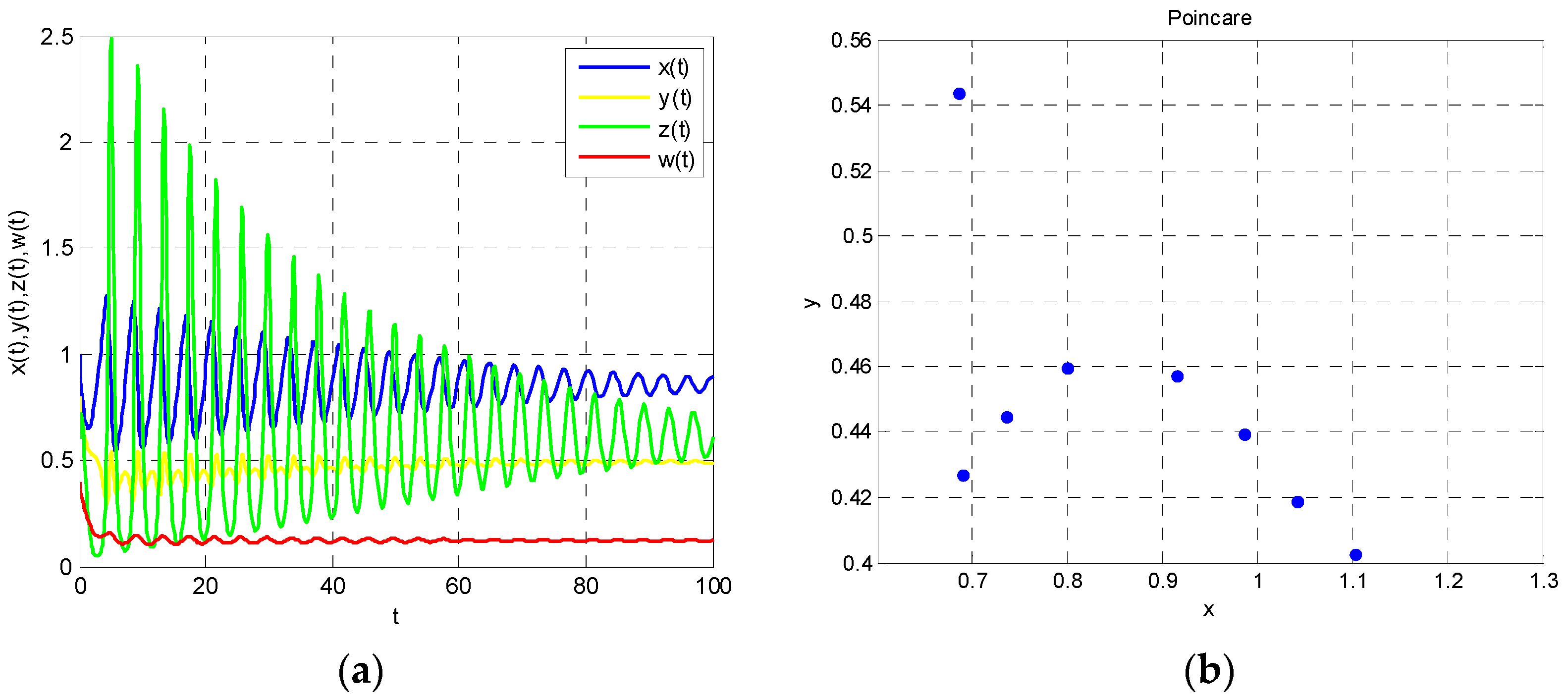
From Theorem 1, we also know that Model (22) is unstable when ${\tau }_1=0.4>{\tau }_{10}=0.2208,{\tau }_2=0$. At this time, Poincare section turns into a semi-circle, which means that the system has periodic solution. That is to say, $x(t)$, $y(t)$, $z(t)$ and $w(t)$ will converge to the basin of attraction through the game. These analyses can be seen in Figure 4 and Figure 5. We conclude that energy demand and energy imports in east China, energy supply in west China and the use of renewable energy is cyclical, which is not conducive to the formulation of long-term energy policy.

Figure 4. (a) Time-domain plot; and (b) Poincare section when ${\tau }_1=0.4>{\tau }_{10}=0.2208$, ${\tau }_2=0$.

Figure 5. The attractor when ${\tau }_1=0.4>{\tau }_{10}=0.2208$, ${\tau }_2=0$: (a) $x(t),y(t),z(t)$; and (b) $x(t),z(t),w(t)$.

Based on the above analysis, we know that system stability must be ${\tau }_1<{\tau }_{10}$. In other words, hydroelectric power stations must shorten the time of water storage. Therefore, we can take the following measures: on the one hand, we can increase the capacity for water storage in rainy seasons; and, on the other hand, the excess energy should be converted to water storage.

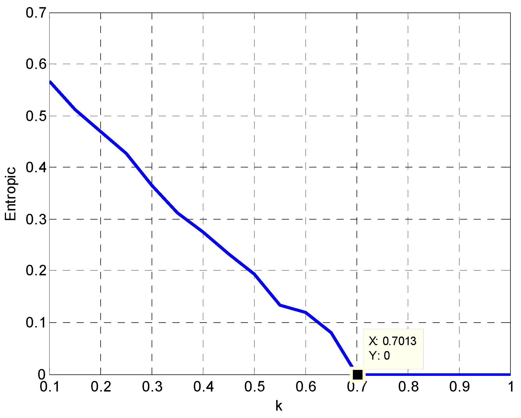
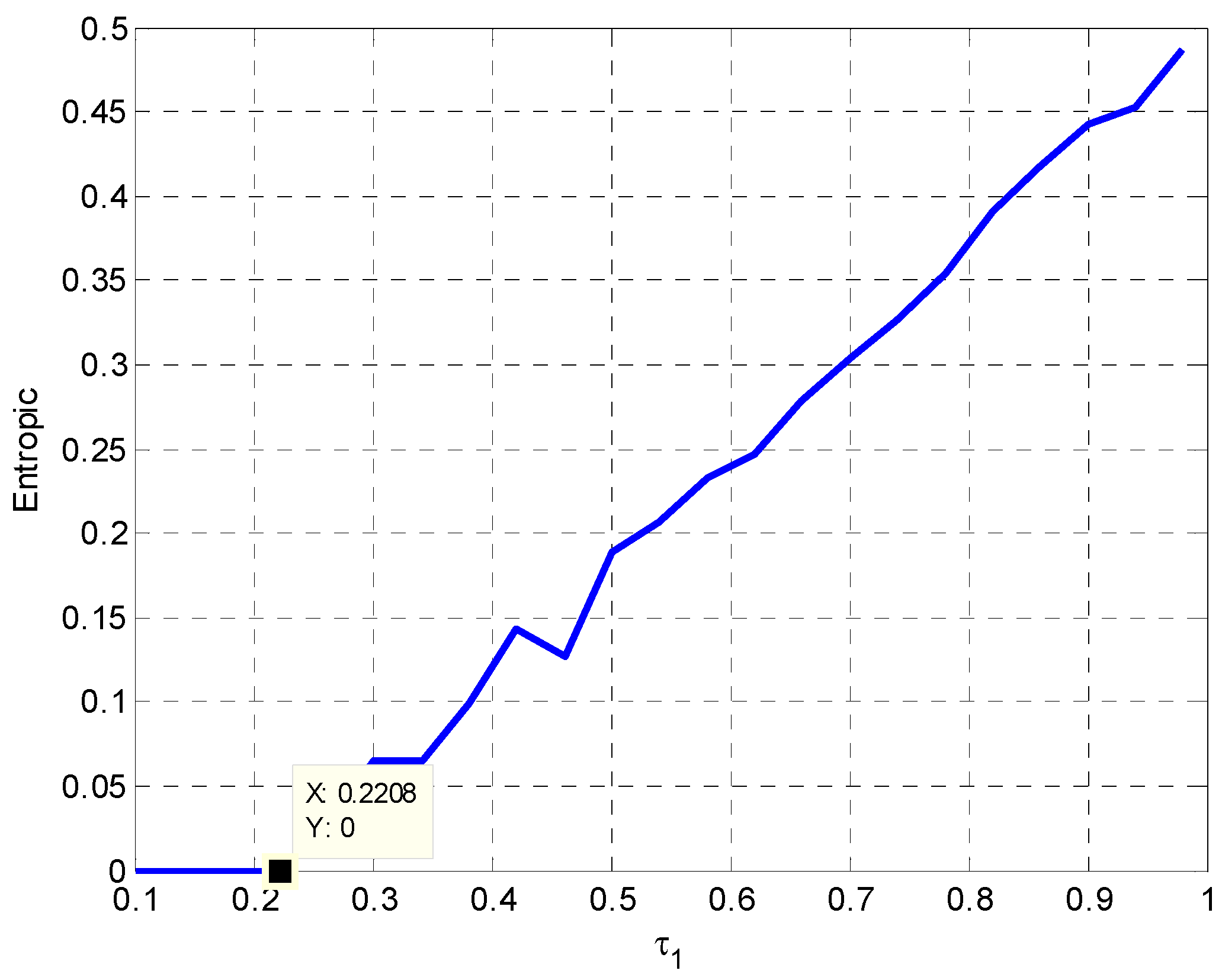
3.2. The Influence of ${\tau }_1$ on the Entropy of Model (22)

Entropy is a measure of the complexity of the system. The greater entropy represents the more complex system. Let the entropy value be $k$. If the system is stable and in regular motion, then the value of $k$ is equal to 0. Otherwise, it is greater than 0. Based on the analysis in Section 3.1, we know that $k=0$ when ${\tau }_1<{\tau }_{10}=0.2208$ or $k>0$ when ${\tau }_1>{\tau }_{10}=0.2208$. Entropy becomes bigger with the increase of ${\tau }_1$ when ${\tau }_1>{\tau }_{10}=0.2208$. Namely, the system becomes more and more complex. In this complex system, energy supply and coordination will be even more difficult. At this point, it will take longer or be more difficult for the system to return to the stable state. The change trend of entropy is displayed in Figure 6.

Figure 6. The entropy plot respect to ${\tau }_1$ when ${\tau }_2=0$.

3.3. The Influence of ${\tau }_1,a_1,d_3$ on the Stability of Model (22)

In Figure 7, it can be found that the impact of $a_1$on $x$ is relatively obvious. However, the impact of ${\tau }_1$ on $x$ is weak. There is an obvious fluctuation of $x$ with the increase of $a_1$. In this process, the minimum value of $x$ is −1.573 × 10¹³ for $({\tau }_1,a_1)=(1,0.05)$, and the maximum value of $x$ is 8.701 × 10¹¹ for $({\tau }_1,a_1)=(0.25,0.65)$. The analysis shows that the energy consumption coefficient $a_1$ has the greatest impact on the energy demand when other parameters are fixed. Therefore, the unscientific energy consumption coefficient will affect the accuracy of the energy demand forecast and further impact the social and economic development.

Figure 7. The influence of ${\tau }_1$ and $a_1$ on $x$ when ${\tau }_2=0$.

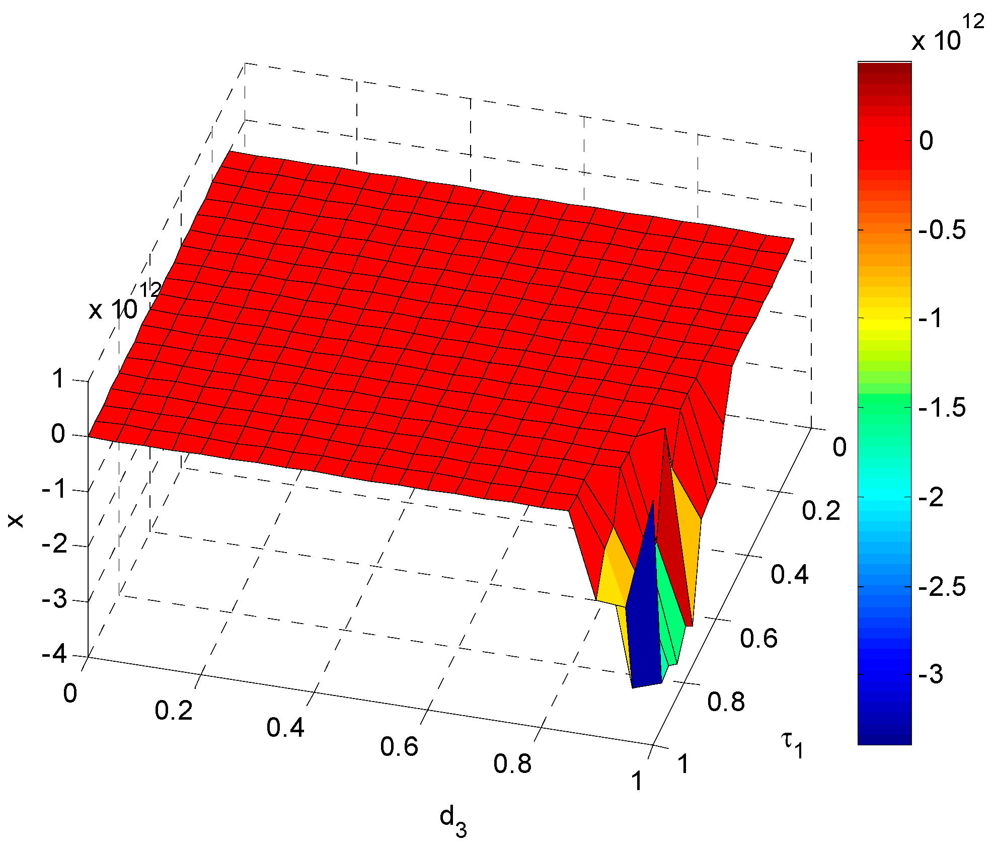
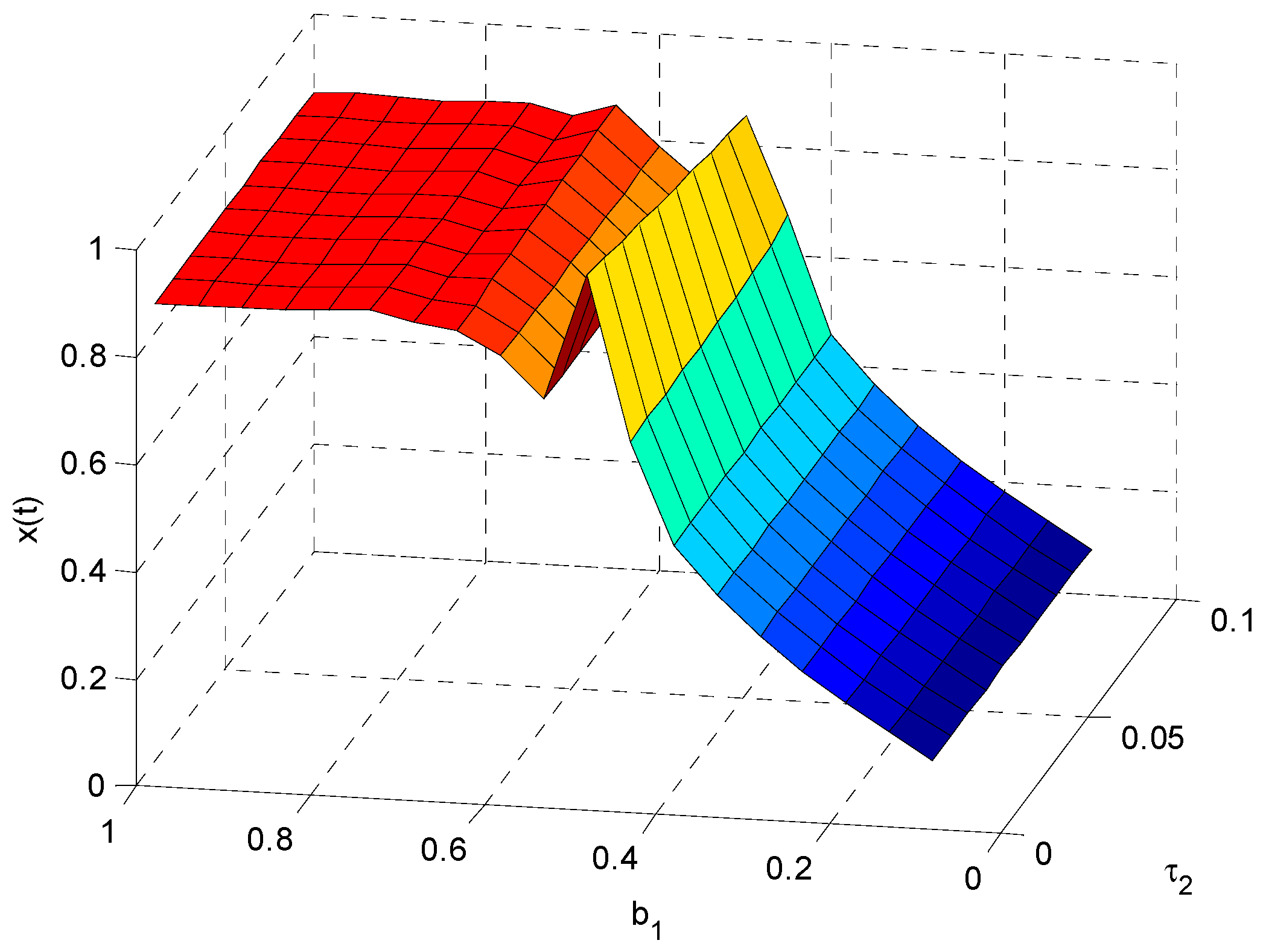
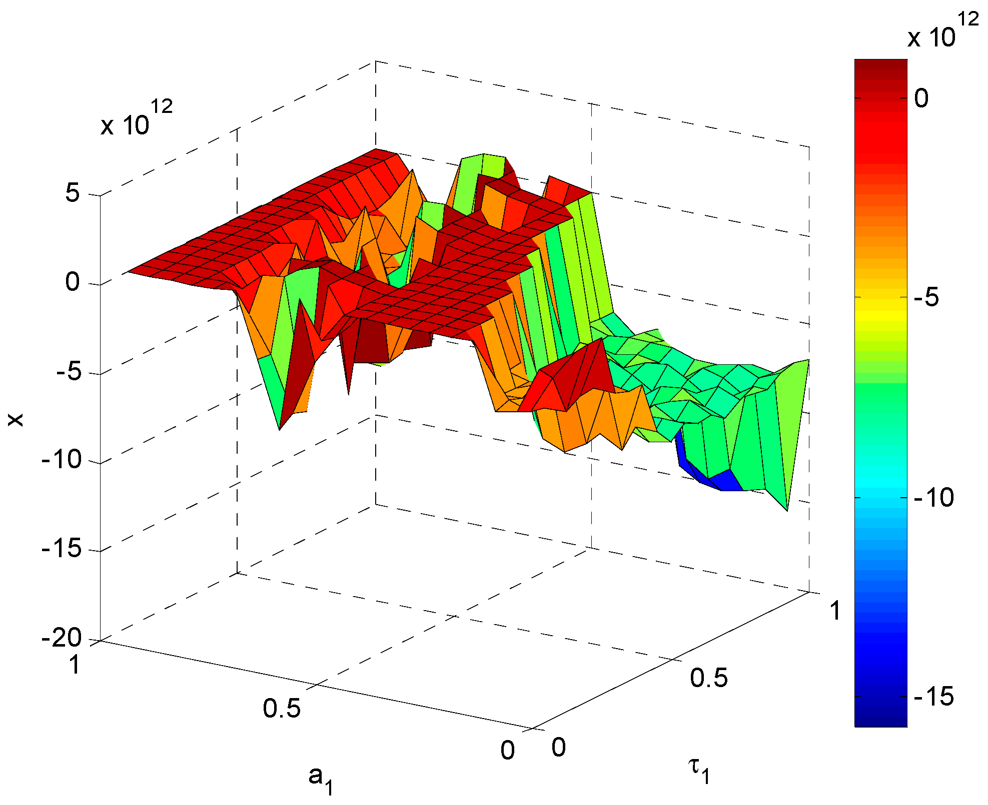
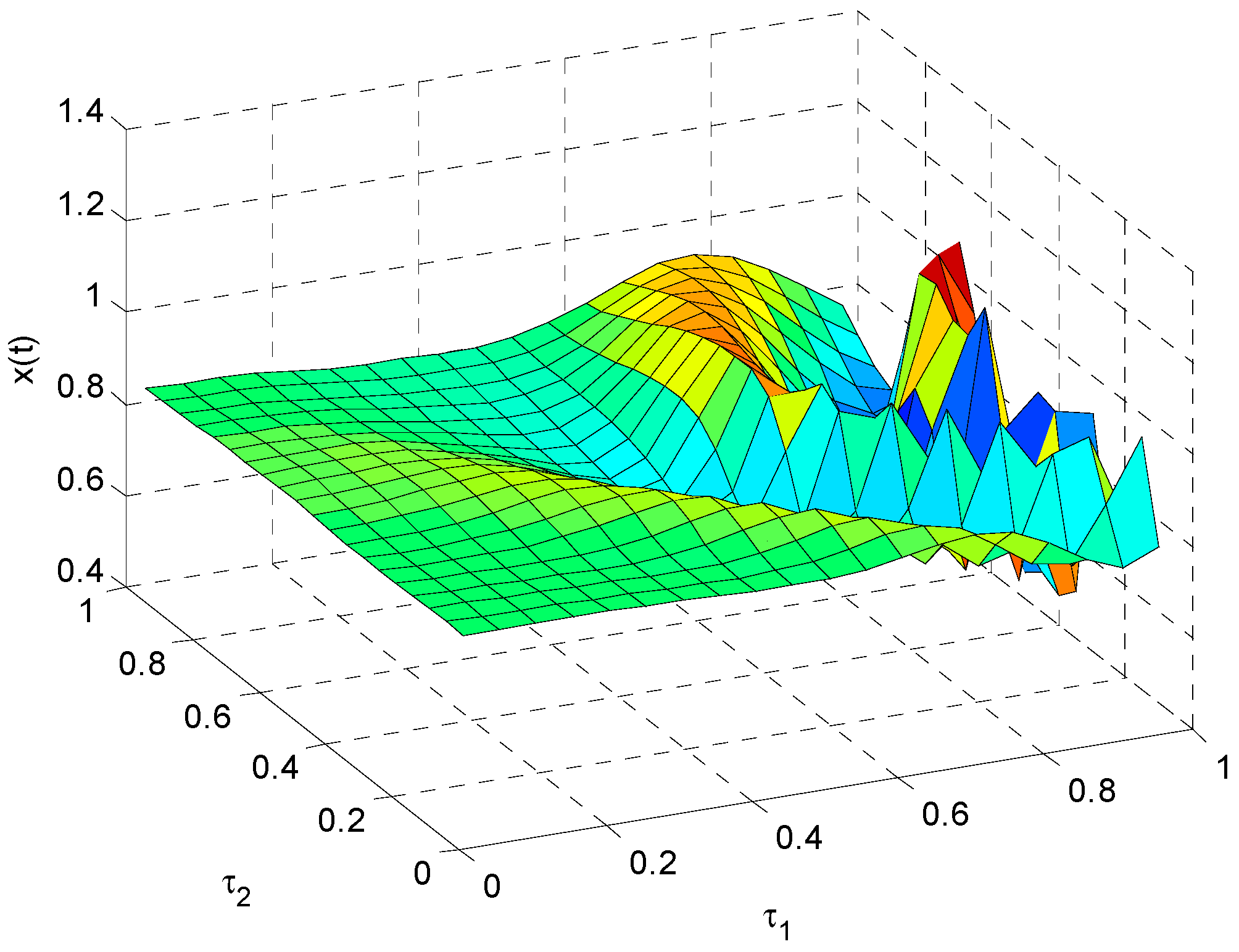
In Figure 8, we can see that $x$ is stable in most region of ${\tau }_1$ and $d_3$. In this unstable region, the minimum value of $x$ is −3.387 × 10¹² for $({\tau }_1,d_3)=(0.85,1)$, and the maximum value of $x$ is 4.387 × 10¹¹ for $({\tau }_1,d_3)=(1,1)$. The $x$ is approximately 0.85 in stable regions. If the other parameters are unchanged, we must ensure ${\tau }_1<0.5$ or $d_3<0.85$ in order to maintain the stability of energy demand.

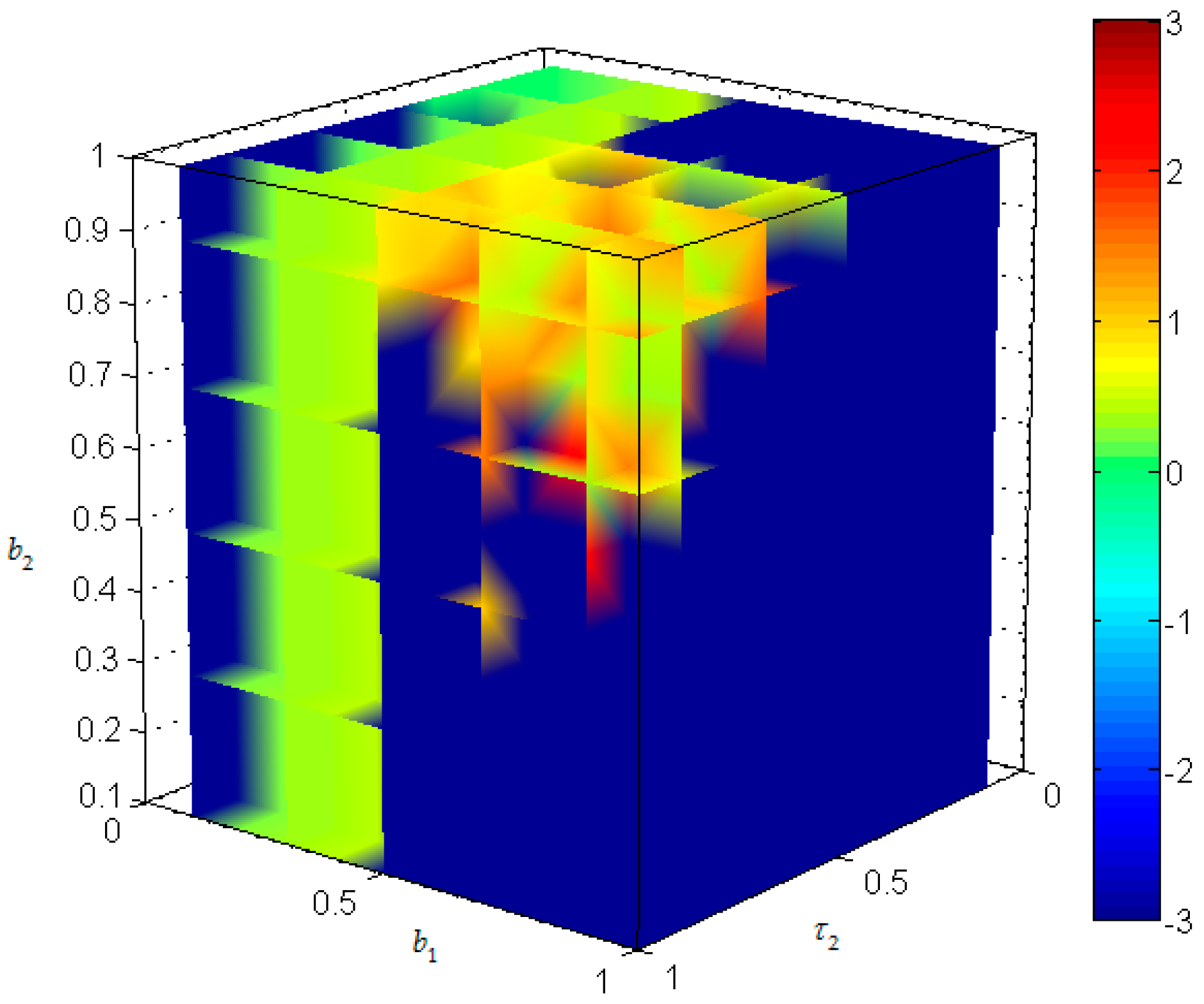
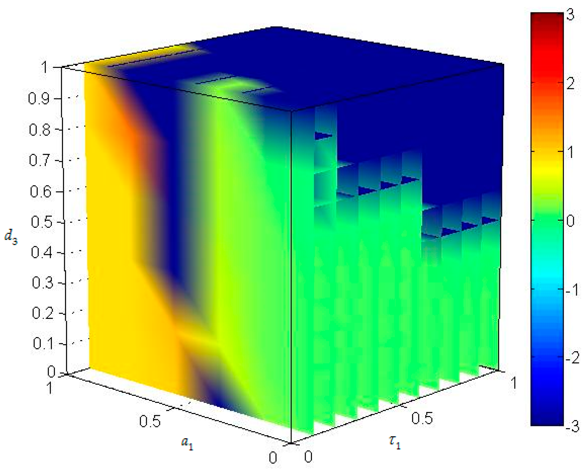
Figure 8. The influence of ${\tau }_1$ and $d_3$ on $x$ when ${\tau }_2=0$.

When $d_3<0.5$, ${\tau }_1$ has little effect on $x$, and the value of $x$ shifts from small to large with the increase of $a_1$. When $d_3>0.5$, $x$ shifts from large to small with the increase of ${\tau }_1$ and there is larger fluctuation with the increase of $a_1$. In order to maintain the stability of energy supply–demand system, we must ensure $d_3<0.5$, $a_1$ close to 1 or 0 and ${\tau }_1>0$. The game relationship among three parties can be observed in Figure 9.

Figure 9. The influence of ${\tau }_1,a_1$ and $d_3$ on $x$ when ${\tau }_2=0$.

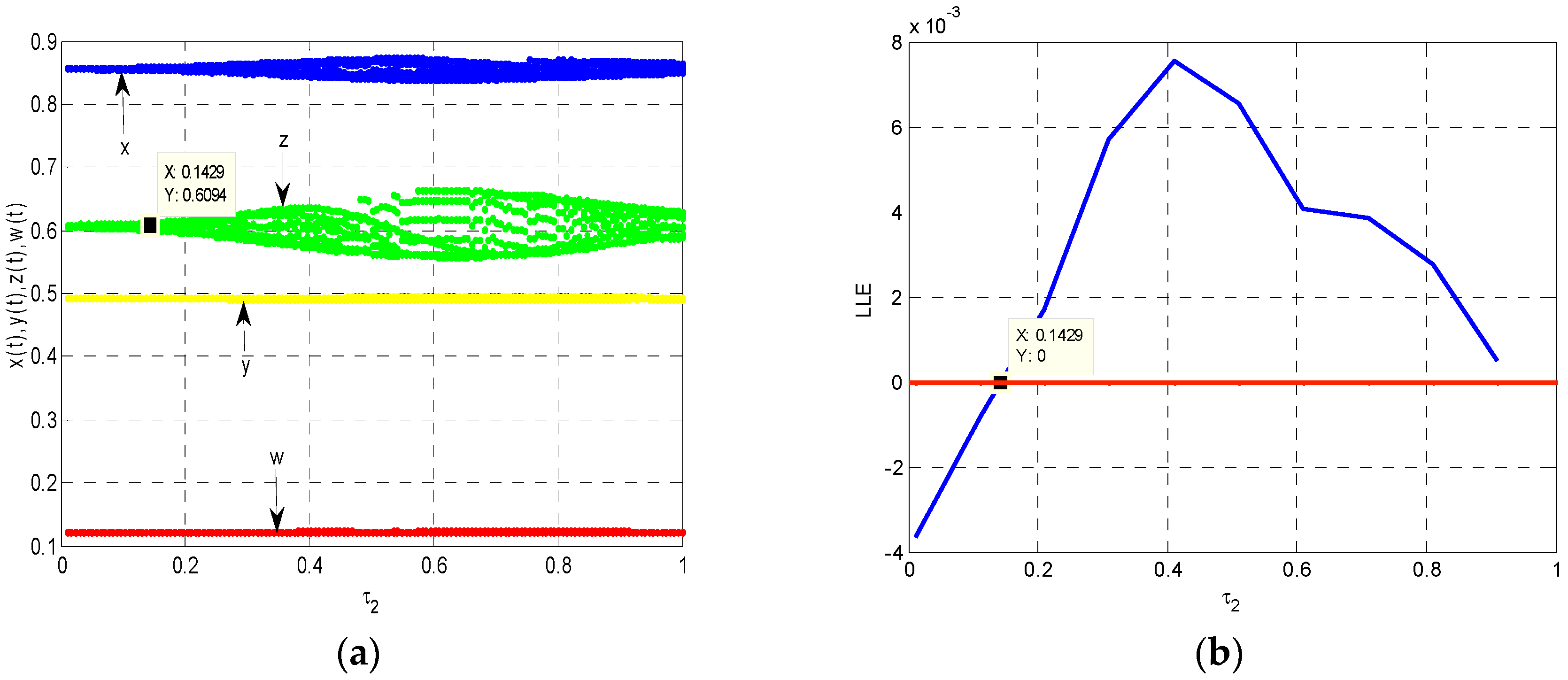
3.4. The Influence of ${\tau }_2$ on the Stability of Model (22)

Let ${\tau }_1=0.1\in [0,{\tau }_{10})$, we study the impact of ${\tau }_2$ on the stability of the system. Model (22) will become unstable with the increase of ${\tau }_2$. Figure 10a displays the dynamic evolution process of Model (22). Similar to Section 3.1, Figure 10b shows that Model (22) undergoes bifurcation at ${\tau }_2=0.1429$ for ${\tau }_1=0.1$. Therefore, the simulation results are in agreement with the theoretical analysis. From the above analysis we can find that the energy demand and energy imports show fluctuations when ${\tau }_2>0.1429$, so we must shorten the time of energy supply in west China. Comparing Figure 1 and Figure 2, we find that the change of ${\tau }_1$ or ${\tau }_2$ would cause $x(t)$ and $z(t)$ fluctuations. Therefore, we should focus on energy imports strategy.

Figure 10. The influence of ${\tau }_2$ on the stability of Model (22) when ${\tau }_1=0.1$: (a) bifurcation diagram; and (b) the largest Lyapunov exponent plot.

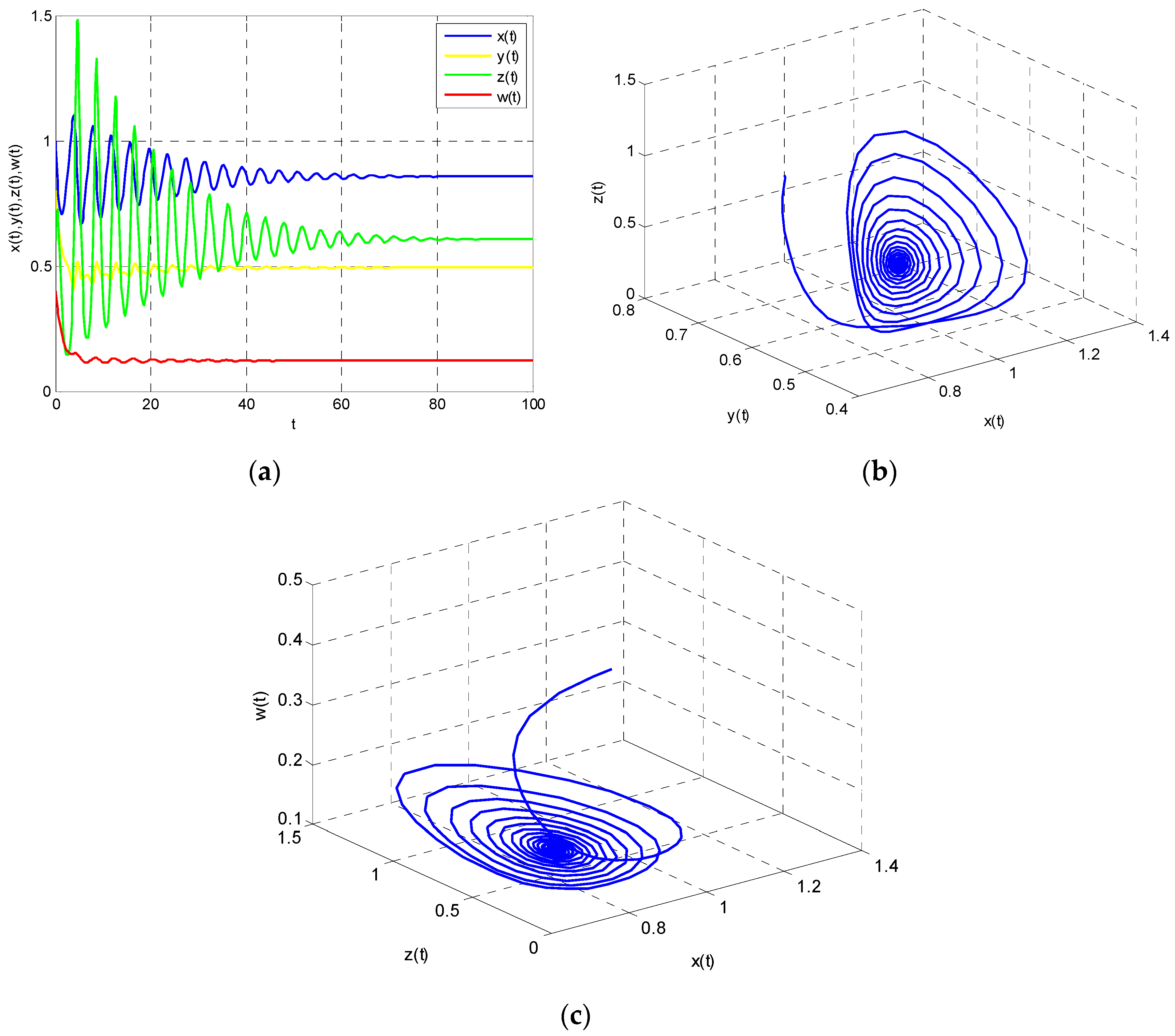
According to Theorem 2, Model (22) is stable when ${\tau }_1=0.1,{\tau }_2=0.05<{\tau }_{20}=0.1429$. Figure 11a shows that each participant of the system has taken the best strategy through game. Finally, the system will be in a stable state. Hence, $x(t)$, $y(t)$, $z(t)$ and $w(t)$ will converge to the equilibrium point $E(0.8572,0.4929,0.6088,0.1225)$. These properties are shown in Figure 11b,c. If the system is stable, it means that energy demand and energy imports are invariable when other parameters are fixed. It is beneficial to formulation and implementation of the energy policy.

Figure 11. The influence of ${\tau }_2$ on the stability of Model (22) when ${\tau }_1=0.1,{\tau }_2=0.05<{\tau }_{20}=0.1429$: (a) Time-domain plot; (b) energy supply–demand attractor $(x(t),y(t),z(t))$; and (c) energy supply–demand attractor $(x(t),z(t),w(t))$.

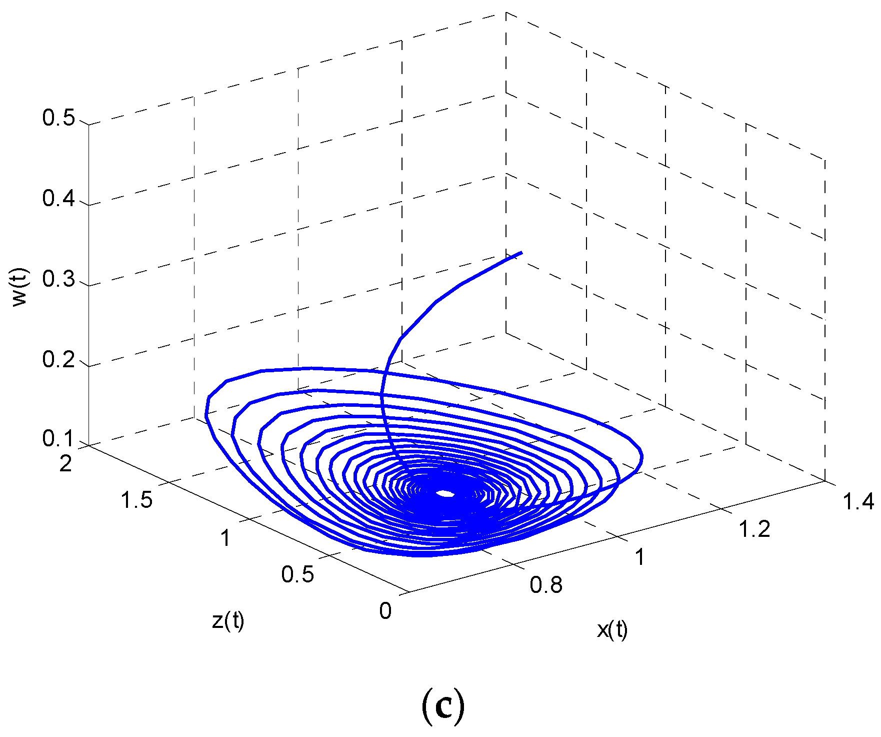
Based on Theorem 2, Model (22) is unstable when ${\tau }_1=0.1,{\tau }_2=0.35>{\tau }_{20}=0.1429$. Figure 12a shows the dynamic game process of each participant in the system. The energy demand and energy imports continue to be in a state of volatility as time goes by, but the fluctuation amplitude decreases. The $x(t)$, $y(t)$, $z(t)$ and $w(t)$ will converge to the basin of attraction through the game. They are in a state of periodic. These characteristics are shown in Figure 12b,c. In this case, it will increase the complexity of energy supply–demand system.

Figure 12. The influence of ${\tau }_2$ on the stability of Model (22) when ${\tau }_1=0.1,{\tau }_2=0.35>{\tau }_{20}=0.1429$: (a) Time-domain plot; (b) energy supply–demand attractor $(x(t),y(t),z(t))$; and (c) energy supply–demand attractor $(x(t),z(t),w(t))$.

3.5. The Influence of ${\tau }_2,b_3,b_4$ on the Stability of Model (22)

In Figure 13, we find that $b_1$ has an obvious impact on , which causes the system to be unstable, but ${\tau }_2$ has no effects on $x$. $x$ suddenly changes from small to large with the increase of $b_1$, and it tends to be stable through slight fluctuations. Finally, $x$ is stable at around 0.8. In the whole evolution process, the maximum value of $x$ is 0.9542 for $({\tau }_2,b_1)=(0.01,0.5)$ and the minimum value of $x$ is 0.0857 for $({\tau }_2,b_1)=(0.1,0.1)$. There are no great ups and downs of $x$ when $b_1>0.5$. In other words, the impact of the speed of energy supply in west China on the energy demand in east China is small.

Figure 13. The influence of ${\tau }_2$ and $b_1$ on $x$ when ${\tau }_1=0.1$.

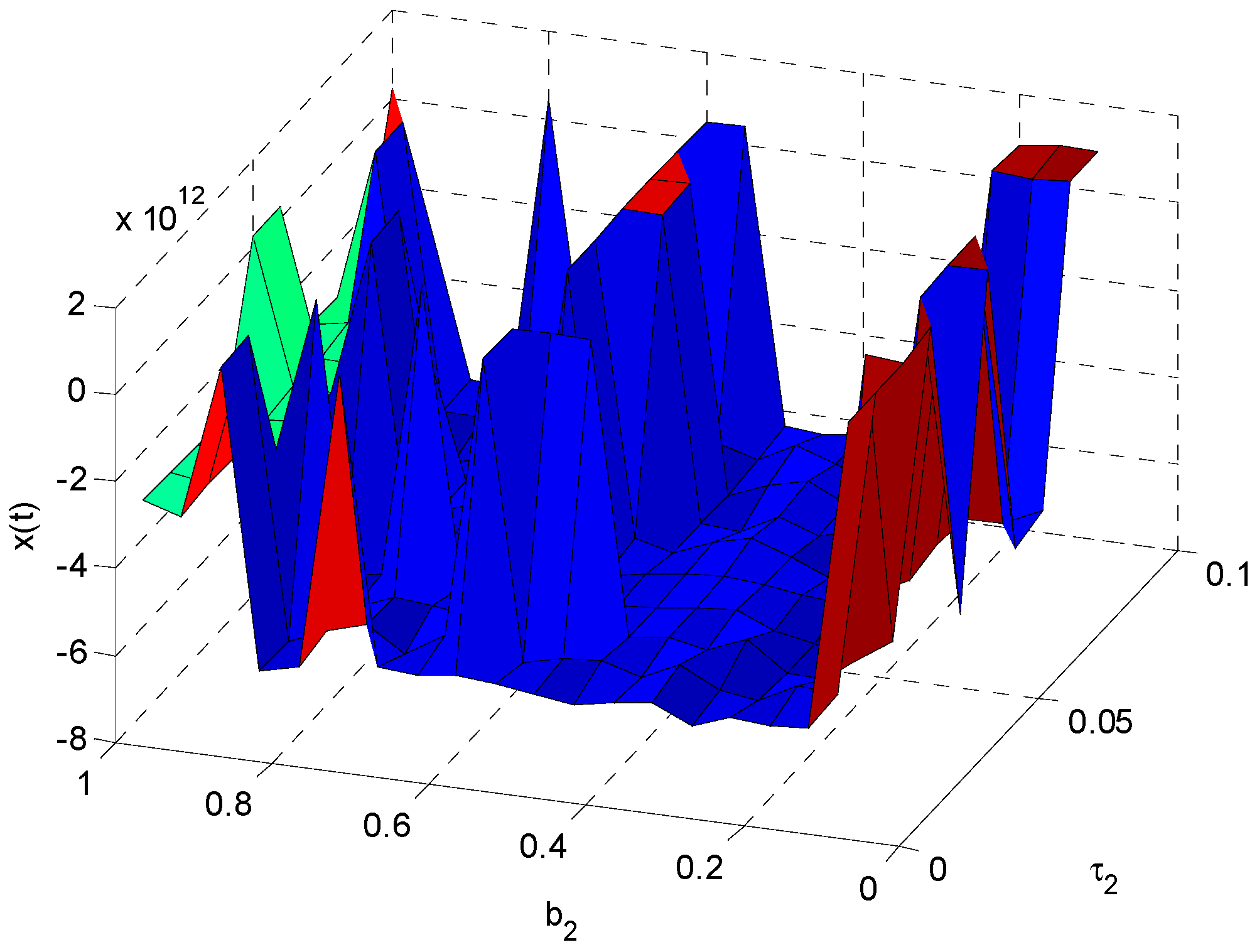
The impact of $b_2$ on $x$ is larger, which causes large $x$ fluctuations. Although the influence of ${\tau }_2$ on $x$ is smaller, it also leads the instability of $x$. The maximum value of $x$ is 9.558 × 10¹¹ for $({\tau }_2,b_2)=(0.09,0.2)$ and the minimum value of $x$ is −6.97 × 10¹² for $({\tau }_2,b_2)=(0.04,0.2)$. Most regions of $({\tau }_2,b_2)$ plane are stable at approximately 6 × 10¹². The above features are shown in Figure 14.

Figure 14. The influence of ${\tau }_2$ and $b_2$ on $x$ when ${\tau }_1=0.1$.

When $b_1<0.5$, $b_2$ has no effect on $x$. When $b_1>0.5$ and ${\tau }_2>0.5$, the value of $x$ becomes larger with the increase of $b_2$. However, $b_2$ has no impact on $x$ when $b_1>0.5$ and ${\tau }_2<0.5$. When $b_2<0.6$, ${\tau }_2$ has no impact on $x$ and the $x$ moves from small to large and again to small with the increase of $b_1$.When $b_2>0.6$, $x$ shifts from small to large with the increase of ${\tau }_2$ and there is fluctuation with the increase of $b_1$. These properties can be seen in Figure 15.

Figure 15. The influence of ${\tau }_2,b_1$ and $b_2$ on $x$ when ${\tau }_1=0.1$.

3.6. The Influence of ${\tau }_1,{\tau }_2$ on the Stability of Model (22)

When ${\tau }_1>0.4$, the amplitude of fluctuation of $x$ is larger. If the ${\tau }_1$ and ${\tau }_2$ are smaller, $x$ is more stable, and it is stable at about 0.47. In unstable region, the maximum value of $x$ is 1.179 for $({\tau }_1,{\tau }_2)=(0.86,0.31)$ and the minimum value of $x$ is 0.5637 for $({\tau }_1,{\tau }_2)=(0.96,0.26)$. The change trends are shown in Figure 16. If you want to get the energy demand accurately, you must make sure that ${\tau }_1$ and ${\tau }_2$ are in a smaller region. Otherwise, the system will be unstable.

Figure 16. The influence of ${\tau }_1$ and ${\tau }_2$ on $x$.

4. Bifurcation Control

According to the above analysis, we know that if the system is unstable, it will lead to fluctuations of the system and increase the complexity of the system. Thus, it is necessary to take measures to ensure the system is in a stable state. In this paper, we implement bifurcation control by using the method of delayed feedback control [24]. Thus, we study the following bifurcation control system:

$$\{\begin{array}{l}\frac{dx}{dt}=x(1-\frac{x}{3.8})-0.6x(y(t-{\tau }_2)+z)-0.8w(t-{\tau }_1)+k(w(t-{\tau }_1)-w),\\ \frac{dy}{dt}=-y-1.2z+1.5x[1.2-(x-z)],\\ \frac{dz}{dt}=11z(0.7x-0.6),\\ \frac{dw}{dt}=0.1x-0.7w,\end{array}$$

(23)

We realize the effective bifurcation control by adjusting the control parameter $k$. Referring to the conclusion in Section 3.1, we know that if ${\tau }_1=0.4,{\tau }_2=0$ Model (22) is unstable and becomes more complex with the increase of ${\tau }_1$. It can be seen in Figure 4, Figure 5 and Figure 6.

4.1. Bifurcation Value

Figure 17a shows that the dynamic evolution process of Model (23) for ${\tau }_1=0.4,{\tau }_2=0$. According to Figure 17b, we obtain that Model (23) has a bifurcation at $k=0.7013$. That is to say, Model (23) is unstable when $k<0.7013$ and it is stable when $k>0.7013$, which means that the control parameter $k$ can affect the stability of the system. In Figure 17a, we find that the greater control parameter $k$ is, the better control effect is. Otherwise, it is the other way around.

Figure 17. The influence of $k$ on the stability of Model (23) when ${\tau }_1=0.4,{\tau }_2=0$: (a) bifurcation diagram; and (b) the largest Lyapunov exponent plot.

4.2. Model (23) Is Unstable

Let $k=0.6<0.7013$, the time-domain plot and attractor of Model (23) are displayed in Figure 18. We find that Model (23) is still unstable and it has a basin of attractor. This is consistent with the above analysis. That is, the control parameter does not play any role in bifurcation control.

Figure 18. Model (23) is unstable when $k=0.6<0.7013$ for ${\tau }_1=0.4,{\tau }_2=0$: (a) time-domain plot; (b) energy supply–demand attractor $(x(t),y(t),z(t))$; and (c) energy supply–demand attractor $(x(t),z(t),w(t))$.

4.3. Model (23) Is Stable

Let $k=0.8>0.7013$, the time-domain plot and attractor of Model (23) are shown in Figure 19. We can see that Model (23) returns to a steady state. Therefore, bifurcation control is successful as $k>0.7013$.

Figure 19. Model (23) is stable when $k=0.8>0.7013$ for ${\tau }_1=0.4,{\tau }_2=0$: (a) time-domain plot; (b) energy supply–demand attractor $(x(t),y(t),z(t))$; and (c) energy supply–demand attractor $(x(t),z(t),w(t))$.

4.4. The Influence of Control Parameter $k$ on Entropy

When $k<0.7013$ the system is unstable, entropy is more than 0. If $k>0.7013$, the system is stable, then entropy is equal to 0. This phenomenon is shown in Figure 20. Thus, it can reduce the complexity of the system by adjusting the control parameter $k$, which indicates that the system will get rid of the unstable state and return to the stable state.

Figure 20. The entropy plot about $k$ when ${\tau }_1=0.4,{\tau }_2=0$.

We conclude that the energy supply–demand system will be unstable if these uncertain factors are added, but it will regain the stable state if delay feedback control method is administered.

5. Conclusions

In this paper, a four-dimensional energy supply–demand model with two-delay is built. We study the impacts of delays and other parameters on the stability of the system. The change of parameters will result in the system switching between stability and instability. In order to keep the stability of the system, we must ensure that the value of delays is less than the bifurcation value or the combination of delays and other parameters in the stable region. Otherwise, the system will go through huge fluctuations. It will be difficult to formulate energy scheduling policy. Therefore, we can carry out bifurcation control by the delayed feedback control method for the unstable system. The system returns to a stable state by adjusting control parameters.

The research results show that the delays play an important role in the stability of the system. With other conditions unchanged, we must take steps to minimize the time delay. For example, to improve the storage capacity of hydropower stations to ensure sustained and stable power output; if there is interruption, there should be timely replenishment to restore power generation, so it must be ensured that ${\tau }_1<0.2208$. In addition, to improve the transport capacity of coal resources in west China to shorten the transport time and to avoid excessive delay-caused supply interruption for the eastern coal demand, it must be ensured that ${\tau }_2<0.1429$. According to the research presented in this paper, we conclude that $d_3<0.85$ for ${\tau }_1>0$, ${\tau }_2=0$ and $b_1>0.5$ for ${\tau }_1=0.1$, ${\tau }_2>0$ can keep the system in stable state other parameters being unchanged.