Article

Intra-Day Trading System Design Based on the Integrated Model of Wavelet De-Noise and Genetic Programming

1
Department of Industrial and Systems Engineering, The Hong Kong Polytechnic University, Hong Kong 999077, China
2
School of Government, Beijing Normal University, Beijing 100875, China
*
Author to whom correspondence should be addressed.
Entropy 2016, 18(12), 435; https://doi.org/10.3390/e18120435
Submission received: 13 October 2016 / Revised: 24 November 2016 / Accepted: 1 December 2016 / Published: 6 December 2016
(This article belongs to the Collection Advances in Applied Statistical Mechanics)

Abstract

:
Technical analysis has been proved to be capable of exploiting short-term fluctuations in financial markets. Recent results indicate that the market timing approach beats many traditional buy-and-hold approaches in most of the short-term trading periods. Genetic programming (GP) was used to generate short-term trade rules on the stock markets during the last few decades. However, few of the related studies on the analysis of financial time series with genetic programming considered the non-stationary and noisy characteristics of the time series. In this paper, to de-noise the original financial time series and to search profitable trading rules, an integrated method is proposed based on the Wavelet Threshold (WT) method and GP. Since relevant information that affects the movement of the time series is assumed to be fully digested during the market closed periods, to avoid the jumping points of the daily or monthly data, in this paper, intra-day high-frequency time series are used to fully exploit the short-term forecasting advantage of technical analysis. To validate the proposed integrated approach, an empirical study is conducted based on the China Securities Index (CSI) 300 futures in the emerging China Financial Futures Exchange (CFFEX) market. The analysis outcomes show that the wavelet de-noise approach outperforms many comparative models.

1. Introduction

Technical analysis related studies have been extensively conducted by researchers and investors for decades in various financial domains.Technical trading rules are generated from historical price and volume data, buying and selling signals are usually sent to exchanges over a very short time period. To beat the market, many machine learning tools have been utilized in the design of technical trading systems. For linear analysis of the financial time series, one of the most commonly used tools is the genetic programming.
Genetic programming (GP) is an automated method for creating a working computer program from a high-level problem statement of a problem. In this paper, GP is used to find the optimized combinations of technical indicators that are capable of generating profit from the market. Past researchers have applied GP into the design of trading systems. However, their models are all trained with a long-term period of data, such as daily, weekly or even monthly data. One of the largest drawbacks of these kinds of systems is that the incoming information effect is not considered. Information, such as financial reports and change of interest rates, are highly likely to affect the price movement of the target analyzing asset—jumping points occurred after the announcement of such information. GP models trained with long-term data which includes many jumping points are unable to extract the real characteristics of the time series. To overcome this problem, in this paper, all the models are trained using the intra-day data. Information that has a dramatic impact on the market is expected to be digested during the market closed periods, therefore, jumping points barely existed in the intra-day data. True trends of the time series can be recognized with GP models trained using the intra-day data.
Another innovation point of this paper is the noise reduction of the intra-day data. High frequency intra-day financial time series are highly correlated and unstationary. Wavelet de-noise is applied in this paper to handle the noises. Wavelet transformation leads to a sparse representation for many real-world signals, and many features in different scales of the data can be localized. Wavelet transformation concentrates the signal in a few large-magnitude wavelet coefficients. Wavelet coefficients which are small in value are typically noise and can be removed while preserving important signal features. Both the soft-thresholding and the hard-thresholding methods are used in this paper to de-noise data. Optimized GP models based on the original data and the proposed wavelet de-noised data are compared with each other using the out-of-sample performance.
In this paper, the CSI 300 index future is selected as the target training and testing asset. The index future market of China is one of the most actively traded emerging markets. Past studies on index futures usually use the frequency of a day, a week or even a month, some of which indeed showed outstanding performance in the out-of-sample experiments. However, these kinds of theoretical profits are highly unrealistic in the real markets; that is because most of the trades in the future markets are margin trading and small movements of the stock index might lead to a large amount of gains or losses to the investors. For most of the time, investors do not have enough money to wait for the market to go to the right price that their model expected. The proposed model in this paper is trained using the intra-day 1-minute interval data. For each trading day, the data is separated into two different parts: the first part is used to train the GP model and the second part is used to perform the out-of-sample performance. In this way, no open position is held overnight, which could greatly reduce the risk caused by overnight unfavorable price jumps.
The remainder of this paper is organized as follows. Relevant studies are briefly reviewed in Section 2. In Section 3, the wavelet de-noise and genetic programming based approach are elaborated and the design of the experiment is explained. Section 4 presents the empirical experiment. This paper concludes in Section 5.

2. Literature Review

2.1. Technical Analysis

Technical analysis is a broad class of methods and strategies that exploit the short-term fluctuation of the security prices. Historical price and volume data are analyzed to generate trading rules to profit from the markets. Although the results in the 1960s and 1970s supported the “efficient market hypothesis”, which indicate that financial markets are efficient and that no excess return can be gained based on the study of past data [1,2], the results since the 1980s showed that successful trade based on the application of technical analysis could be made [3,4,5,6]. Despite the fact that it has been criticized and scorned by many academic researchers, technical analysis has proved itself to be useful and powerful in both academia and practice. Gencay, Fernandez-Rodrıguez and Chavarnakul [7,8,9] presented extensive reviews on the relevance of technical analysis in financial markets and the profitability of a technical pattern. Taylor and Allen [10] reported that up to 90 percent of traders use some sort of technical analysis in their practical trading. Recently, technical indicators such as MA (moving average), and MACD (Moving Average Convergence/Divergence) are commonly used in the analysis of stock price movement.

2.2. Genetic Programming

Evolutionary algorithms such as genetic programming allow a system to automatically generate and adapt trading rules according to certain criteria. Developed by [11], genetic algorithms were combined with technical trading rules. Bauer [12] reported that systems built based on genetic algorithms were able to generate positive excess returns in the US exchange market. However, genetic programming was argued to be more appropriate in extracting trading rules from historical data because of its special structure [13]. A flexible framework for adjusting the trading rules to the current environment was presented in [14]. With the application of genetic programing to the financial industry, researchers tested its capability of generating excess returns using a data set from different markets and different assets. Chen and Yeh [15] and Allen and Karjalainen [16] failed in their attempts to generate excess returns over buy-and-hold approaches on stock indexes. However, Neely [17,18] and Marney [19] found otherwise, at least when the notion of risk is not considered.
Furthermore, Potvin et al. [20] tested genetic programming based trading systems with 14 individual stocks listed on the Toronto stock exchange market. Without consideration of the transaction cost, they found out that some systems were profitable, while others may suffer heavy losses. By taking the transaction cost into consideration, Mallick et al. [21] and Esfahanipour et al. [22] reported positive excess return over buy-and-hold strategies in the markets, the genetic programming generated trading rules were able to beat the popularly used MACD technical indicator. Straßburg et al. [23] proposed the parallelization to improve the generation of technical trading rules by speeding up the computing and enabling more results. Hongguang and Ping [24] tested the performance of genetic programming systems with the China index future market. Luengo et al. [25] separated the market into three market scenarios, including bull market, bear market and sideways markets. They found that strategies based on genetic programming perform the best in the sideways market. Combined with a fuzzy system, genetic algorithms were used to select stock from certain markets to form a better portfolio [26]. Hu et al. [27] presented a detailed literature review on the evolutionary algorithmic trading.

2.3. Applications of Wavelet in Financial Analysis

Over the past two decades, many researchers applied the wavelet method to finance and economic fields. Large amounts of financial and econometric investigations have been conducted with the application of wavelet in various areas. According to [28], four major aspects are covered in these applications. In this research, the forecasting of time series is the only concern and, hence, in this subsection, forecasting related wavelet literature is briefly reviewed. Some basic and mathematical literature about wavelets can be found in [29,30,31,32]. A short-term load forecasting was conducted using wavelet transformation (WT) [33], in which the Daubechies wavelet transforms were adopted to identify the load characteristics in electric systems. The proposed model was proved to have good performance in the load prediction of three-hour intervals. Sandoval and Hernandez [34] utilized the WT in the analysis of order book volume dynamics. Zhang et al. [35] investigated the effectiveness of WT to improve financial time series forecasting. In this study, a three stage prediction scheme, namely, the decomposition, the multi-layer perceptron and the recombination, was proposed. The shining point of this study is the utilization of the realistic money management system and trading model to evaluate the forecasting performance. With the proposed forecasting model, the trading system was proved to be more profitable, which makes it one of the most convincing empirical experiments. Similarly, Zhang et al. [35] and Renaud et al. [36] utilized the wavelet decomposition for forecasting short (short-term movement) and long (trend) memory of the time series. An Auto Regressive (AR) multi-scale model was proposed and tested with both simulated and real-world data and the forecasting results were shown to outperform the neural network (NN) based approaches. They concluded that a linear mapping of the multi-resolution data is more stable than more sophisticated nonlinear alternatives. Schleicher et al. [37] were among the first to present a full practical introduction to wavelets for economists, in which some basic ideas and related economic applications of the wavelet were illustrated. Crowley [38] improved the work in [37] by adding more examples of applications and more detailed explanations about different wavelets and wavelet transforms. Furthermore, they provided various software sources and a practical guide for researchers to follow their empirical experiment. Yousefi et al. [39] utilized the WT to investigate the market efficiency of crude oil futures markets. The Discrete Wavelet Transform (DWT) was used to decompose the oil price into different time scales. Different models were assigned to each time scale to fit the characteristic of the data, after which the final forecasting results were achieved by the wavelet construction. The empirical results indicated that the wavelet-based forecasting procedure performed the best for large sample sizes, which makes it extremely suitable for high-frequency short-term stock index forecast. Li et al. [40] designed a hybrid forecasting model by the combination of genetic programming and wavelet decomposition. Different scales of the decomposition of the original stock index were chosen as indicators to feed the financial genetic programming (FGP) model. The proposed model was used to predict whether the Dow Jones Industrial Average Index (DJIA) will rise by 2.2 percent or more within the next 21 trading days. Significant improvement of forecasting performance was observed compared to the conventional FGP. Stolojescu et al. [41] tested a wavelet based forecasting method for time series. In this study, four prediction methodologies, including Artificial Neural Networks (ANN), Autoregressive Integrated Moving Average (ARIMA), linear regression and the random walk model were combined with the Stationary Wavelet Transform (SWT). Different mother wavelets were also applied in the decomposition process of the original data. The ANN method was shown to have the best performance compared to the rest. In the Master’s thesis of Chong Tan (2009), an intensive introduction and review of NN and WT were presented. A hybrid wavelet de-noising based forecasting model was designed to fulfill the prediction task. In their model, the SWT and the DWT were compared to show the impact of shift-invariant. The proposed model was then utilized to forecast a bunch of exchange rates, whose performance was shown to beat the benchmark models in a short-term forecast. It also demonstrates the feasibility of combing wavelet NN and statistical methods, which might be modified to conduct high frequency short-term financial series forecasting.

2.4. Intra-Day Trading System

Most intra-day trading decisions are made by computerized quantitative models. High-frequency trading, commonly defined as quantitative trading, is characterized by extreme short portfolio holding periods. Kirilenko et al. [42] explored the impact of the intra-day trading and analyzed the reason for the flash crash in 2010. Kablan and Falzon [43] introduced the Sugeno model in the implementation of the ANFIS (Adaptive Neuro-Fuzzy Inferences Systems) to forecast a high-frequency financial time series and to estimate parameters. In their research, Kablan developed a system that performs a prediction on the financial times series in high frequency using intra-day data (5-min intra-day trading prices). Buy and sell orders are placed based on the predication of the movement of the prices. Their system was observed to have a very high accuracy rate on opening the right position at the right place.

3. Methodology

3.1. Wavelet and Wavelet De-Noise

To overcome the shortcomings of the Fourier transform in the performing of a multi-resolution analysis of signals, the wavelet has been widely applied in different fields. Unlike the Fourier analysis, wavelets are localized in both time and frequency scale. Mathematically, a wavelet is defined as a function with a zero average:
ψ ( t ) d t = 0
The concept of WT is to represent the target function as a superposition of a set of wavelets which are small waves located at different times. The original series can be transformed and described in the content of a different frequency over time at a certain time-scale. Wavelet-based models are suitable for non-stationary data as some transient trends or hidden characteristics of the original series can be highlighted. Financial time series are well-known to be non-stationary, which makes WT one of the most powerful tools for the analysis and forecasting of financial time series.

3.1.1. The Discrete Wavelet Transform

For the most practical studies, wavelet coefficients are not needed to be calculated at every possible scale as it would be a fair amount of work to do that, which will generate an awful lot of data. The DWT projects a time series onto a collection of orthonormal transformations. Unlike the continuous wavelet transformation that considers all possible frequencies at continuous times, the DWT focuses on some specific frequencies at distinct times. The discrete wavelet is defined as:
ψ j , k ( t ) = S 0 1 j ψ ( t k τ 0 S 0 j S 0 j )
j and k are integers. S 0 > 1 is a fixed dilation step and the translation factor τ 0 depends on the dilation step. If S 0 = 2 , the discrete wavelet transformation is defined as a dyadic wavelet transform. By definition, the scaling function and the wavelet function of discrete wavelet transformation are:
φ ( 2 j t ) = i = 1 k a k φ ( 2 j + 1 t k )
Equation (3) is the scaling function, known as the scaled father wavelet, a k are the corresponding coefficients, k ϵ Z . The mother wavelet ψ is obtained by the linear combinations of the scaled father wavelet. Proper coefficients must be selected to maintain the orthogonality of the basis wavelets.
ψ ( 2 j t ) = i = 1 k b k φ ( 2 j + 1 t k )
The mother wavelets ψ are uniquely determined by their coefficients { b k } , k ϵ Z . Then, a signal f ( t ) can be written as:
f ( t ) = i = 1 k a j , k φ ( 2 j + 1 t k ) + i = 1 k b j , k ψ ( 2 j + 1 t k )
This is the basic idea of discrete wavelet decomposition of the signal.

3.1.2. Wavelet De-Noise

Separating noises from the original signal is the procedure of de-noise. Suppose f ( t ) is the original time series, some parts of the series s ( t ) represent the trending of the original series, while the others are just localized noises. Then, the model of the de-noise process is :
s ( t ) = f ( t ) e ( i )
e ( i ) represents the noise series. The main steps to perform wavelet de-noise on the financial time series are:
  • Decomposition of the financial time series;
  • Selection of the decomposed part based on wavelet coefficients;
  • Reconstruction of the time series using the selected decomposed part of the original series. The dropped part of the original series is treated as noise that should be removed from this process.
In this paper, the discrete wavelet decomposition is used to decompose the original financial time series, in this way, the most important process of de-noising the original time series becomes to adjust the coefficients of the different decomposed scales. The most commonly used method is the threshold rule.
The basic idea of the threshold rule is to truncate the insignificant coefficients of the decomposed scales of the original time series since less information is contained or only localized noise is contained. One of the key steps is how to select threshold parameters. If the threshold value is less than the noise level, unexpected noises are present in the processed series. However, if the threshold value is significantly bigger than the noise level, the information contained in the original series would be lost. A universal threshold value is proposed by [44] as follows:
t h r e s h o l d = σ 2 l o g ( N )
σ is the standard deviation and N refers to the total number of the data sets.
There are two kinds of threshold methods, namely the hard threshold and the soft threshold. Both of these methods will be conducted in this research to evaluate the performance with each other. The hard threshold is a straight forward technique to implement the wavelet de-noising process. The advantage of the hard threshold is that it is easy to use and it better reconstructs discontinuities. The coefficient adjustment is given as,
H ( t , d ) = d , i f | d | t 0 , o t h e r w i s e
d represents the wavelet coefficients and t is the threshold value. This method is not a continuous mapping method, and the input coefficients are effective if it is less than or equal to the threshold.
The soft threshold is another way to adjust the wavelet coefficients. Instead of forcing wavelet coefficients to zero or leaving them untouched, the soft threshold pushes all coefficients towards zero, which can be defined as,
S ( t , d ) = d , i f | d | < t S i g n ( d ) ( | d | t ) , o t h e r w i s e
S i g n ( d ) = 1 , i f d > 0 0 , i f d = 0 1 , i f d < 0
Compared with the hard threshold, the different setting happens when the absolute value of wavelet coefficients is greater than the threshold. As all the coefficients are affected in this process, the soft threshold is a continuous mapping method. As all wavelet coefficients are suppressed by the soft threshold, a smoother reconstructed time series is expected. After the control of the wavelet coefficients, de-noised time series is reconstructed using the selected coefficients and scales. In the experiment below, both the original financial time series and the wavelet de-noised time series will be used separately in the calculation of technical indicators to train the genetic programming model. The performance of the resulted trading systems will be compared with each other.

3.2. Generating Trading Rules with Genetic Programming

In this subsection, the process to conduct the adaptation of genetic programming is presented. The genetic programming will be used to generate trading rules based on technical indicators which are encoded as programs.

3.2.1. Encoding of the Technical Indicators

The initial programs, which are represented as tree structures, are recursively constructed from a predefined set of functions F and Terminals T. Both functions F and Terminal T change dynamically during the evolution process. Functions F and Terminal T are defined in the following [20]:
  • Functions:
    • Arithmetic operators: +, −, *, /;
    • Boolean operators: a n d , o r , n o t ;
    • Relations operators: <, >;
    • Boolean functions: if-then-else.
    • Real functions (user defined functions, here are the technical indicators)
  • Technical Indicators, Variable s Represents Constant Price:
    • N o r m ( r 1 , r 2 ) : absolute value of the difference between real number;
    • A v g ( s , n ) : average of price over the past n periods;
    • E M A ( s , n ) : exponential moving average of the past n periods;
    • M a x ( s , n ) : maximum value of price over the past n periods;
    • M i n ( s , n ) : minimum value of price over the past n periods;
    • L a g ( s , n ) : price value lagged by n periods;
    • V o l a t i l i t y ( n ) : variance in returns over the past n periods;
    • R S I ( n ) : relative strength index;
    • R O C ( n ) : rate of change.
      R O C ( n ) = ( closing price of the current minute closing price of n minutes ago 1 ) × 100
      R S I ( n ) = 100 ( 100 1 + R S ( n ) ) : R S ( n ) = i D + ( n ) r i i D ( n ) r i , D + is the set of minutes with rising prices, D is the set of minutes with falling prices and r i is the return of minute i, which is positive when the price is rising and negative otherwise.
  • Terminals:
    • Constants: chosen in the interval [ 0 , 270 ] , where 270 is the approximate number of minutes in a single trading day;
    • Boolean: True, False;
    • Others: Price
    • Real variable: P price of the current minute;
    • Order Types: Entry order and Exit order
    • Entry order: Market Entry order: enter into the market at market price;
    • Stop Entry order: these orders are placed above the market for a long entry and below the market for a short entry;
    • Limit Entry order: these orders are placed below the market for a long entry and above the market for a short entry;
    • Exit order: Exit at target profit, Exit at target percentage profit, Exit at Target price, Protective Stop, Trailing Stop, Exit after N Bars, Exit after N Bars profit, Exit after N Bars loss, Exit after certain time, Exit at Market, Exit End-of-Day.
It is obvious that functions and terminals sets chosen in this research violate the closure assumption of genetic programming. Some of the function sets cannot disagree with another function in F, given that both Boolean and real functions are found in that set. The restrictions mean that the real functions are always in the lower part of the tree structures. It makes sense that all the trading decisions are made based on technical indicators while Boolean functions and relational operators are found in the upper part of the tree.

3.2.2. Fitness Evaluation Criteria

In most of the relevant studies, fitness values are calculated using the excess return over the markets. However, the net profit is a much more simple and efficient way to evaluate the profitability of trading strategies. In the trading period, the total net profit is the total profit (gross profit minus gross loss) for all closed trades, both profits and losses.

3.2.3. Initialization of the Base Population

There are two methods to generate the initial population of the trading blocks. The full method creates tree structures, in which the length of every path between a terminal and the root equals to a predefined depth. The growing method creates the tree structures with variable shapes. In this paper, a combination of the full and grow methods is applied. Due to the particular structure of the function set, the recursive construction has to follow the rules bellow. Firstly, the root of the tree should be selected from the Boolean functions and operators. It illustrates that the buy and sell signal must be generated at the top of the tree structure. Secondly, descendants of the tree can be selected among Boolean constants, Boolean functions, Boolean or Boolean operators. Thirdly, a relational operator’s descendants should be selected among real functions or terminals.
After the generation of the initial population, more complex trading decisions are built using the initial trade blocks with some mutations and crossover.

3.2.4. Crossover, Mutation, Reproduction and Selection

As the initialized populations usually have low fitness, genetic operators must be utilized to search better programs.
The crossover operator is used to combine the genetic material of two parents by swapping a part of one parent with a part of the other. In this paper, the offspring resulting from crossover replaces the parent with less fitness. The mutation operator is used to operate on only one individual. Whenever one of the individuals in a particular population has been selected for mutation, a tree node is selected randomly and the existing sub-tree is replaced with a randomly created sub-tree. The mutated individual is then put back to the original population to calculate the fitness. The reproduction operator is simply a clone of the current tree structure, which usually happens to a tree with a rather high fitness value. This operator is controlled by the parameter reproduction probability.
In the selection of programs in the population, a ranking based approach proposed by Baker (1985) and Whitley (1981) is used. To use the ranking system, the fitness of all programs must be calculated and sorted from the best (rank 1) to the worst (rank N). A new value f i is then associated with the program or rank i as follows:
f i = M a x [ ( M a x m i n ) i 1 N 1 ]
In this way, the best program gets fitness M a x , and the worst program gets fitness M i n . Most importantly, the remaining programs are equally spaced between M i n and M a x . The super program problem that crowded out all the other programs can be avoided.

3.3. Design of the Experiment in This Paper

The designed genetic programming method will be applied to the original financial time series and the wavelet de-noised time series. The detailed process is shown in Figure 1.
Three experiments are conducted simultaneously. In the first experiment, technical indicators are calculated using the original 1-minute frequency data of the CSI 300 index future. After that, genetic programming will be used to search for the best possible combinations of all the indicators and order types listed in the methodology. Once the optimized trading strategies are determined for each trading day, out-of-sample tests of the models are conducted. One of the key points in the design of these experiments is that all the technical indicators are calculated using the data from a single trading day and no historical trading information of the former day or before is used in the calculation of the indicators. It is a good try to reduce the effect of price jump between two trading days. In the second experiment, the original data will firstly be de-noised with two different methods, namely the soft threshold and hard threshold wavelet de-noise method. Both the initialized population and the technical indicators will be re-calculated using the de-noised data. After that, the de-noised data will be used to calculate the related indicators. The rest of the second experiment is similar to the first experiment. Furthermore, to explore the effect of different trading day jumps, another experiment is conducted. In the last experiment, multiple days of data will be used instead of the single day data in the training of the models. The overall trading results of the third experiment will be compared with the first and second experiment.

4. Empirical Experiment

In this empirical experiment, the CSI 300 Index future is selected as the target asset. Detailed information about the index future is shown in the following Table 1. A total of 21 days of the CSI 300 index future data are used, each of which contains 270 data points. The original data points cover the period from 29 September 2014 to 3 November 2014. The training and testing data used in this paper are selected very carefully. From 29 September 2014 to 9 October 2014, there is a slightly upward trend; from 13 to 20 October 2014, the index almost hovers laterally and from 21 to 27 October 2014, there is a clearly downward trend. Three different kinds of trading environment are covered in this experiment. In each trading day, the first 128 data points are used to train the model, and the last 142 data points will be used to test the out-of-sample performance of the model. A total of 128 training data points are selected by the decomposition requirement of the wavelet analysis. As the morning session of a trading day consists of 130 min, the training processes were conducted in the morning session and the out-of-sample testing process was conducted in the afternoon session. For both the training and testing of the GP model, an initial value of 100,000 CNY is invested in the portfolio; for each trading action, only one share of the contract is assumed to be executed without any delay.
To overcome the over-fitting problem, a higher weight is assigned on the out-of-sample performance of the developed model. Only the out-of-sample performances will be discussed as the in sample trading profit is highly unrealistic. As shown in the design of the experiment, the out-of-sample performance of the model optimized by the 128 in-sample original data points will be compared with the model optimized by the wavelet, de-noised, 128 in-sample data points. As described in the methodology section, there are two different de-noise methods: the hard threshold and soft threshold. Both methods will be applied in this paper to compare with each other. Another comparative study about the trading with and without holding assets overnight is also tested. In the experiment of holding the assets overnight, the first 14 days of the data are used to train the model, and the last seven days of data are used to test the out-of-sample profitability. Also, just like the first experiment, wavelets will also be utilized to de-noise the in-sample data.

4.1. Parameter Settings

Excessive preliminary experiments were conducted to optimize the parameters for the genetic training process. The guideline of the GP parameters selection is to maximize the sum of the profit for all of the trading days and to reduce time consumption for the total training process. The detailed process is based on trial and error. The limit of entries per day of 8 is the maximum amount of shares of trading that one account can make per day, which is regulated by the government. The max bars looking back for indicators of 30 is selected based on my past program trading experience. The final parameters are illustrated in Table 2.

4.2. Experiment Results

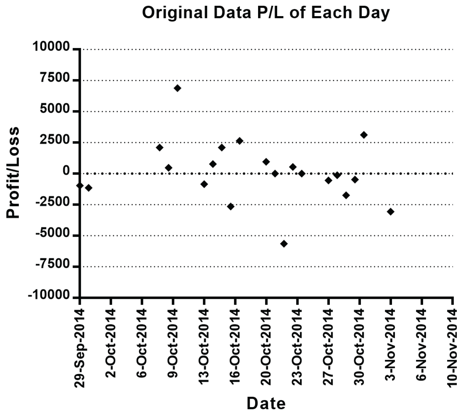
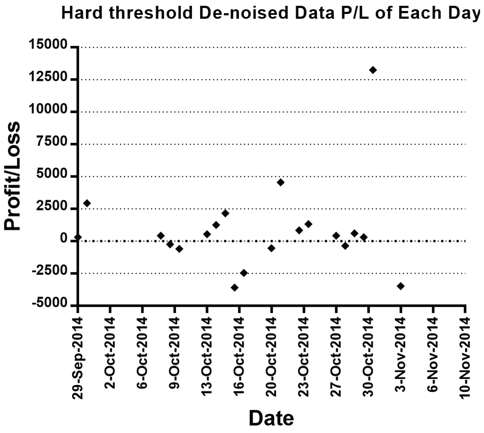
The detailed trading results of 21 days without holding assets overnight are shown in Table 3. As shown in Table 3, the out-of-sample performance of the training models varies during different trading days. The positive value represents gains and the negative value represents losses. The sum of the total trading profits and losses for three different training methods are 2460 for the GP strategy trained on the original data, 11,760 for the GP model trained on the hard threshold wavelet de-noised data and 3720 for the GP strategy trained on the soft threshold wavelet de-noised data.
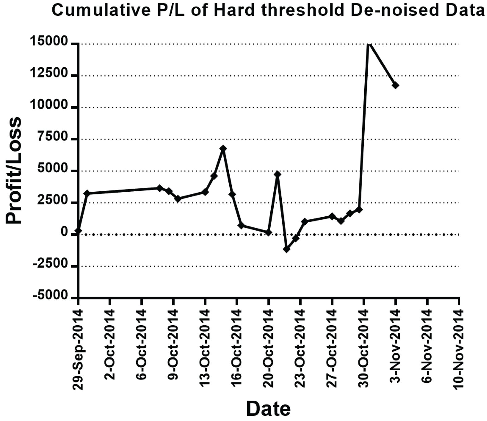
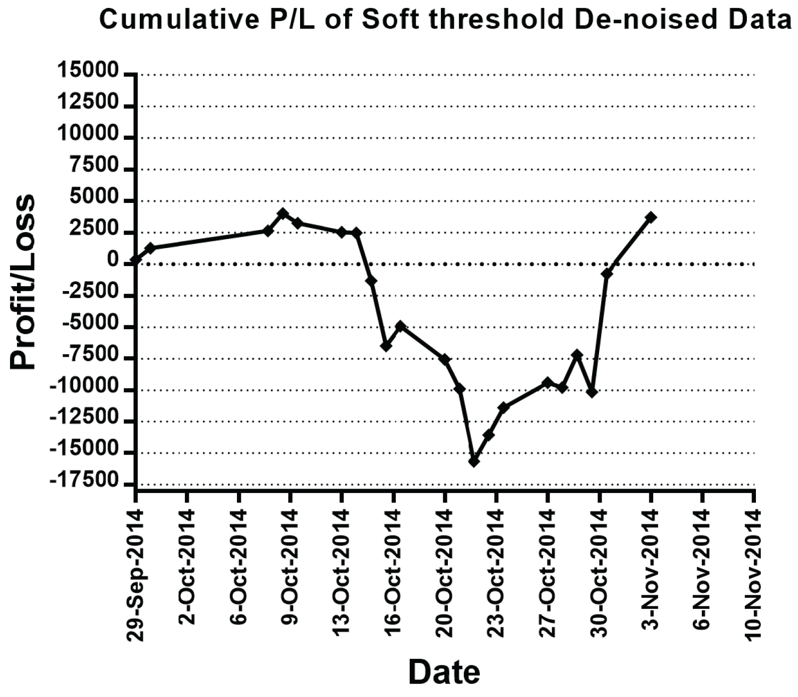
The intra-day training and testing results are shown in Figure 2, Figure 3 and Figure 4. The results in Table 3 indicated that better out-of-sample performance is obtained if the GP model is trained with wavelet de-noised data sets and the hard threshold de-noise method has the best out-of-sample performance. At the bottom of Table 3, the min, max and std of each profit and loss are listed; the results indicate that the max intra-day loss for the three experiments does not vary that much. The hard threshold has the highest possible intra-day loss of 5880. However, it also has the highest possible intra-day profit of 13,260. The soft threshold has a higher possible loss and lower possible profit than the performance from the original data. With a much higher standard deviation of the profit/loss, the out-of-sample results showed an interesting phenomenon that the wavelet de-noise process tends to magnify the gains and losses for most of the trading days. From Figure 5, Figure 6 and Figure 7, it is clear that the hard threshold de-noised data have the lowest max drawdown and the highest possible profit, which made it the best trading strategy in the experiments. Although the soft threshold de-noised data-trained strategy has higher total profit than the original data-trained strategy, the max drawdown is much higher than the other two strategies. Since the initial capital invested is 100,000 CNY, the monthly return of the models are 2.46%, 11.76% and 4.02%; the trading strategy trained with the hard threshold de-noised data have the highest monthly return.
As the total trading profit of the wavelet de-noise data-trained models is higher than the model trained from the original data, it can be concluded that, with the consideration of the non-stationary and noisy characteristics of intra-day high-frequency time series, and the application of wavelet de-noise, better trading performance systems can be developed.
The trading results in Table 4 indicate that when multi-days of data are utilized to train the model, all the out-of-sample trading is subjected to severe losses. Although the performance of the trading system based on the multi-days data is not that comparable to the intra-day trading strategies proposed above as the training and testing periods are not precisely the same. The severe losses in Table 4 indicated that trading trend varies in different trading days and profitable trading strategies in a certain trading day might suffer from severe losses in other days. There is a high possibility that an overfitting problem existed in the optimized model, however, these results also proved that the jumping points in the price of the index future will influence the performance of GP trained models, and that models trained using long time intervals cannot extract the genuine trend of the series, as the jumping points which are caused by exogenous information are more likely to be recognized as significant features than the genuine trend.

5. Conclusions and Future Work

In this research, an integration of the genetic programming and wavelet de-noise are utilized to generate intra-day programmed trading rules. The results showed that the trading rules generated by genetic programming with the wavelet de-noised data points have better out-of-sample performance and that the hard threshold de-noise method outperforms the soft threshold methods. The trading strategies trained with morning session data are most likely to be profitable in the afternoon session of the same trading day. Also, the trading GP strategies trained with multi-days of data may lead to severe losses in the following several trading days, which indicates that the trend of financial time series tends to vary on different trading days and stays the same on a single trading day.
As trading strategies are trained separately using different data from single days, which makes the experiment pretty complex, only 21 days of 1-min data are tested in the experiment; more tests need to be conducted to evaluate the robustness of the GP trained strategies. As the results of the experiments in this paper indicate that the wavelet de-noised data-trained trading system has better performance compared to the original data-trained system, the design of the real-time trading systems proposed in this paper can be summarized as follows: (1) Wavelet de-noise in the morning session 1-min data of the index future; (2) Train the GP model based on the reconstructed data; (3) Trade the index future based on the trained systems in the afternoon trading session. Another potential research area is that, although the trading cost is considered in this paper, much more realistic problems, such as topological execution of orders and the execution delay of orders, should be taken into consideration before the deployment of the actual system.

Acknowledgments

The work described in this paper was partially supported by two grants from The Hong Kong Polytechnic University, China (Project No. G-RTK6 and 4-BCBJ).

Author Contributions

Hongguang Liu, Ping Ji and Jian Jin conceived and designed the experiments; Hongguang Liu collected the data; Hongguang Liu, Ping Ji and Jian Jin performed the experiments; Jian Jin contributed analysis tools; Hongguang Liu wrote the paper. All the authors have read and approved the final manuscript.

Conflicts of Interest

The authors declare no conflict of interest.

References

  1. Alexander, S.S. Price movements in speculative markets: Trends or random walks. Ind. Manag. Rev. 1961, 2, 7. [Google Scholar]
  2. Malkiel, B.G.; Fama, E.F. Efficient capital markets: A review of theory and empirical work. J. Financ. 1970, 25, 383–417. [Google Scholar] [CrossRef]
  3. Pruitt, S.W.; White, R.E. The CRISMA trading system: Who says technical analysis can’t beat the market? J. Portf. Manag. 1988, 14, 55–58. [Google Scholar] [CrossRef]
  4. Brock, W.; Lakonishok, J.; LeBaron, B. Simple technical trading rules and the stochastic properties of stock returns. J. Financ. 1992, 47, 1731–1764. [Google Scholar] [CrossRef]
  5. Bessembinder, H.; Chan, K. The profitability of technical trading rules in the Asian stock markets. Pac. Basin Financ. J. 1995, 3, 257–284. [Google Scholar] [CrossRef]
  6. Sweeney, R.J. Beating the foreign exchange market. J. Financ. 1986, 41, 163–182. [Google Scholar] [CrossRef]
  7. Gencay, R. The predictability of security returns with simple technical trading rules. J. Emp. Financ. 1998, 5, 347–359. [Google Scholar] [CrossRef]
  8. Fernandez-Rodrıguez, F.; Gonzalez-Martel, C.; Sosvilla-Rivero, S. On the profitability of technical trading rules based on artificial neural networks: Evidence from the Madrid stock market. Econ. Lett. 2000, 69, 89–94. [Google Scholar] [CrossRef]
  9. Chavarnakul, T.; Enke, D. A hybrid stock trading system for intelligent technical analysis-based equivolume charting. Neurocomputing 2009, 72, 3517–3528. [Google Scholar] [CrossRef]
  10. Taylor, M.P.; Allen, H. The use of technical analysis in the foreign exchange market. J. Int. Money Financ. 1992, 11, 304–314. [Google Scholar] [CrossRef]
  11. Holland, J.H. Outline for a logical theory of adaptive systems. J. ACM 1962, 9, 297–314. [Google Scholar] [CrossRef]
  12. Bauer, R.J. Genetic Algorithms and Investment Strategies; Wiley: Hoboken, NJ, USA, 1994. [Google Scholar]
  13. Potvin, J.Y.; Bengio, S. The vehicle routing problem with time windows part II: Genetic search. INFORMS J. Comput. 1996, 8, 165–172. [Google Scholar] [CrossRef]
  14. Koza, J.R. Genetic Programming: On the Programming of Computers by Means of Natural Selection; MIT press: Cambridge, MA, USA, 1992. [Google Scholar]
  15. Chen, S.H.; Yeh, C.H. Toward a computable approach to the efficient market hypothesis: An application of genetic programming. J. Econ. Dyn. Control 1997, 21, 1043–1063. [Google Scholar] [CrossRef]
  16. Allen, F.; Karjalainen, R. Using genetic algorithms to find technical trading rules. J. Financ. Econ. 1999, 51, 245–271. [Google Scholar] [CrossRef]
  17. Neely, C.; Weller, P.; Dittmar, R. Is technical analysis in the foreign exchange market profitable? A genetic programming approach. J. Financ. Quant. Anal. 1997, 32, 405–426. [Google Scholar] [CrossRef]
  18. Neely, C.J.; Weller, P.A. Technical trading rules in the European monetary system. J. Int. Money Financ. 1999, 18, 429–458. [Google Scholar] [CrossRef]
  19. Marney, J.P.; Tarbert, H.; Fyfe, C. Technical Trading Versus Market Efficiency—A Genetic Programming Approach. Available online: http://econpapers.repec.org/paper/scescecf0/169.htm (accessed on 1 Decemder 2016).
  20. Potvin, J.Y.; Soriano, P.; Vallée, M. Generating trading rules on the stock markets with genetic programming. Comput. Oper. Res. 2004, 31, 1033–1047. [Google Scholar] [CrossRef]
  21. Mallick, D.; Lee, V.; Ong, Y.S. An empirical study of genetic programming generated trading rules in computerized stock trading service system. In Proceedings of the 2008 International Conference on Service Systems and Service Management, Melbourne, Australia, 30 June–2 July 2008; pp. 1–6.
  22. Esfahanipour, A.; Karimi, B.; Mousavi, S. The profitability of technical trading rules in tehran stock exchange: An application of genetic programming. In Proceedings of the International Symposium on INnovations in Intelligent SysTems and Applications, Trabzon, Turkey, 29 June–1 July 2009.
  23. Straßburg, J.; Gonzàlez-Martel, C.; Alexandrov, V. Parallel genetic algorithms for stock market trading rules. Procedia Comput. Sci. 2012, 9, 1306–1313. [Google Scholar] [CrossRef]
  24. Hongguang, L.; Ping, J. Generating Intraday Trading Rules on Index Future Markets Using Genetic Programming. Int. J. Trade Econ. Financ. 2015, 6, 112. [Google Scholar]
  25. Luengo, S.; Winkler, S.; Barrero, D.F.; Castaño, B. Optimization of trading rules for the spanish stock market by genetic programming. In Current Approaches in Applied Artificial Intelligence; Springer: Cham, Switzerland, 2015; pp. 623–634. [Google Scholar]
  26. Huang, C.F.; Chang, B.R.; Cheng, D.W.; Chang, C.H. Feature selection and parameter optimization of a fuzzy-based stock selection model using genetic algorithms. Int. J. Fuzzy Syst. 2012, 14, 65–75. [Google Scholar]
  27. Hu, Y.; Liu, K.; Zhang, X.; Su, L.; Ngai, E.; Liu, M. Application of evolutionary computation for rule discovery in stock algorithmic trading: A literature review. Appl. Soft Comput. 2015, 36, 534–551. [Google Scholar] [CrossRef]
  28. Ramsey, J.B. The contribution of wavelets to the analysis of economic and financial data. Philos. Trans. R. Soc. Lond. A 1999, 357, 2593–2606. [Google Scholar] [CrossRef]
  29. Addison, P.S. The Illustrated Wavelet Transform Handbook: Introductory Theory and Applications in Science, Engineering, Medicine and Finance; CRC Press: Boca Raton, FL, USA, 2002. [Google Scholar]
  30. Walnut, D.F. An Introduction to Wavelet Analysis; Springer: Berlin/Heidelberg, Germany, 2013. [Google Scholar]
  31. Walker, J.S. A Primer on Wavelets and Their Scientific Applications; CRC Press: Boca Raton, FL, USA, 2008. [Google Scholar]
  32. Daubechies, I. Ten Lectures on Wavelets; SIAM: Philadelphia, PA, USA, 1992. [Google Scholar]
  33. Yu, I.-K.; Kim, C.; Song, Y.H. A novel short-term load forecasting technique using wavelet transform analysis. Electr. Mach. Power Syst. 2000, 28, 537–549. [Google Scholar]
  34. Sandoval, J.; Hernandez, G. High-frequency trading strategies using wavelet-transformed order book information and dynamic Bayesian networks. In Proceedings of the 2015 Science and Information Conference, London, UK, 28–30 July 2015; pp. 435–442.
  35. Zhang, B.L.; Coggins, R.; Jabri, M.A.; Dersch, D.; Flower, B. Multiresolution forecasting for futures trading using wavelet decompositions. IEEE Trans. Neural Netw. 2001, 12, 765–775. [Google Scholar] [CrossRef] [PubMed]
  36. Renaud, O.; Murtagh, F.; Starck, J.L. Wavelet-Based Forecasting of Short and Long Memory Time Series. Available online: http://www.unige.ch/ses/metri/cahiers/2002_04.pdf (accessed on 1 Decemder 2016).
  37. Schleicher, C. An Introduction to Wavelets for Economists. Available online: http://www.bankofcanada.ca/wp-content/uploads/2010/02/wp02-3.pdf (accessed on 1 Decemder 2016).
  38. Crowley, P.M. An Intuitive Guide to Wavelets for Economists. Available online: https://papers.ssrn.com/sol3/papers.cfm?abstract_id=787564 (accessed on 1 Decemder 2016).
  39. Yousefi, S.; Weinreich, I.; Reinarz, D. Wavelet-based prediction of oil prices. Chaos Solitons Fractals 2005, 25, 265–275. [Google Scholar] [CrossRef]
  40. Li, J.; Shi, Z.; Li, X. Genetic programming with wavelet-based indicators for financial forecasting. Trans. Inst. Meas. Control 2006, 28, 285–297. [Google Scholar] [CrossRef]
  41. Stolojescu, C.; Railean, I.; Lenca, S.M.P.; Isar, A. A wavelet based prediction method for time series. In Proceedings of the 2010 International Conference Stochastic Modeling Techniques and Data Analysis, Chania, Greece, 8–11 June 2010.
  42. Kirilenko, A.A.; Kyle, A.S.; Samadi, M.; Tuzun, T. The flash crash: The Impact of High Frequency Trading on an Electronic Market. Available online: https://papers.ssrn.com/sol3/papers.cfm?abstract_id=1686004 (accessed on 1 Decemder 2016).
  43. Kablan, A.; Falzon, J. The Use of Dynamically Optimised High Frequency Moving Average Strategies for Intraday Trading. World Acad. Sci. Eng. Technol. 2012, 6, 301–307. [Google Scholar]
  44. Donoho, D.; Johnstone, I.; Johnstone, I.M. Ideal Spatial Adaptation by Wavelet Shrinkage. Biometrika 1993, 81, 425–455. [Google Scholar] [CrossRef]
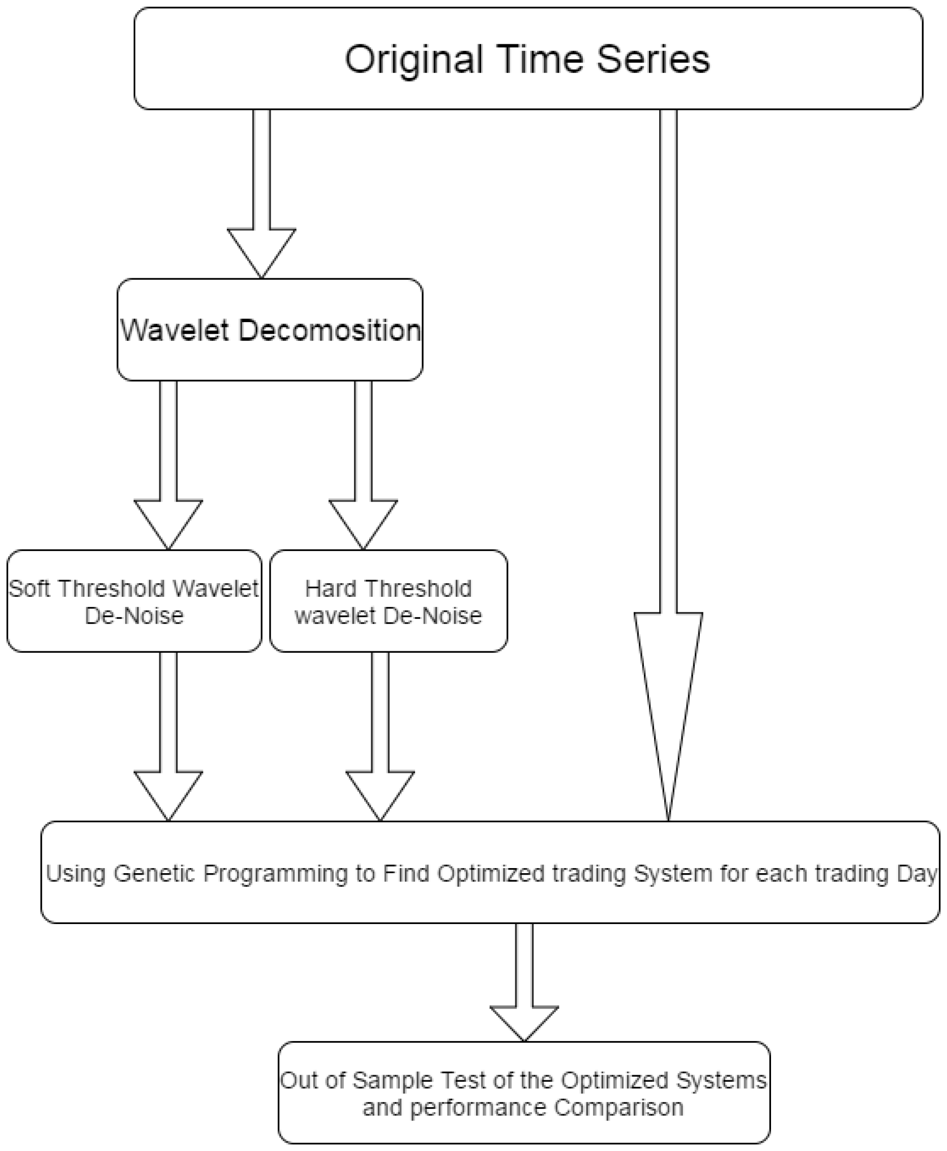
Figure 1. Flow chart of the experiment.
Entropy 18 00435 g001
Figure 2. Original data P/L of each trading day.
Entropy 18 00435 g002
Figure 3. Hard threshold de-noised data P/L of each day.
Entropy 18 00435 g003
Figure 4. Soft threshold de-noised data P/L of each day.
Entropy 18 00435 g004
Figure 5. Cumulative P/L of original data.
Entropy 18 00435 g005
Figure 6. Cumulative P/L of hard threshold de-noised data.
Entropy 18 00435 g006
Figure 7. Cumulative P/L of soft threshold de-noised data.
Entropy 18 00435 g007
Table 1. The CSI 300 Index.
Underlying IndexCSI 300 Index
Contract MultiplierCNY 300
UnitIndex point
Tick Size0.2 point
Contract MonthsMonthly: current month, next month, next two calendar quarters (four total)
Trading Hours09:30 a.m.–11:30 a.m., 01:00 p.m.–03:00 p.m.
Limit Up/Down+/−10% of settlement price on the previous trading day
Margin Requirement8% of the contract value
Last Trading DayThird Friday of the contract month, postponed to the next business day if it falls on a public holiday
Delivery DayThird Friday, same as “Last Trading Day”
Settlement MethodCash Settlement
Transaction CodeIF
ExchangeChina Financial Futures Exchange
Table 2. Parameters for genetic programming.
ParametersValue
Population size300
Number of generations30
Crossover percentage60%
Mutation percentage50%
Tree depth5
Tournament size5
Limit of entries per day8
Wait for exit before entering new tradeYes
Max bars looking back for Indicators30
Table 3. Trading results for 21 days of intra-day data.
DateOut-of-Sample P/L 1 Out-of-Sample Cumulative P/L 2 Out-of-Sample P/L 3 Out-of-Sample Cumulative P/L 4 Out-of-Sample P/L 5 Out-of-Sample Cumulative P/L 6
29 Sep. 2014−960.00−960.00300.00300.00360.00360.00
30 Sep. 2014−1140.00−2100.002940.003240.00900.001260.00
8 Oct. 20142100.000.00420.003660.001380.002640.00
9 Oct. 2014480.00480.00−240.003420.001380.004020.00
10 Oct. 20146900.007380.00−600.002820.00−780.003240.00
13 Oct. 2014−840.006540.00540.003360.00−720.002520.00
14 Oct. 2014780.007320.001260.004620.00−60.002460.00
15 Oct. 20142100.009420.002160.006780.00−3780.00−1320.00
16 Oct. 2014−2640.006780.00−3600.003180.00−5160.00−6480.00
17 Oct. 20142640.009420.00−2460.00720.001560.00−4920.00
20 Oct. 2014960.0010,380.00−540.00180.00−2640.00−7560.00
21 Oct. 20140.0010,380.004560.004740.00−2340.00−9900.00
22 Oct. 2014−5640.004740.00−5880.00−1140.00−5760.00−15,660.00
23 Oct. 2014540.005280.00840.00−300.002100.00−13,560.00
24 Oct. 20140.005280.001320.001020.002160.00−11,400.00
27 Oct. 2014−540.004740.00420.001440.001980.00−9420.00
28 Oct. 2014−120.004620.00-360.001080.00−360.00−9780.00
29 Oct. 2014−1740.002880.00600.001680.002580.00−7200.00
30 Oct. 2014−480.002400.00300.001980.00−2940.00−10,140.00
31 Oct. 20143120.005520.0013,260.0015,240.009360.00−780.00
3 Nov. 2014−3060.002460.00−3480.0011,760.004500.003720.00
Min−5640−2100−5880−1140−5740−15,660
Max690010,38013,26015,24093604020
Std2484NULL3619NULL3313NULL
Out-of-sample Profit/Loss of model trained with original data; 2 Cumulative Profit/Loss of out-of-sample performance of model trained with original data; 3 Out-of-sample Profit/Loss of model trained with hard threshold de-noised data; 4  Cumulative Profit/Loss of out-of-sample performance of model trained with hard threshold de-noised data; 5  Out-of-sample Profit/Loss of model trained with soft threshold de-noised data; 6  Cumulative Profit/Loss of out-of-sample performance of model trained with soft threshold de-noised data.
Table 4. Trading results for multi-day training methods.
DateOut-of-Sample Profit/Loss of Model Trained with Original DataOut-of-Sample Profit/Loss of Model Trained with Hard Threshold De-Noised DataOut-of-Sample Profit/Loss of Model Trained with Soft Threshold De-Noised Data
24 Oct.–3 Nov. 2014−37,320−34,140−22,260