
Modeling of a Mass-Spring-Damper System by Fractional Derivatives with and without a Singular Kernel

 ,
,  and
and 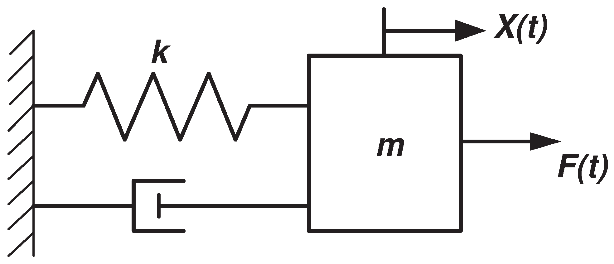
Abstract
:1. Introduction
2. Basic Concepts
3. Mass-Spring-Damper System

- Mass-spring system,and:
- Damper-spring system, :and:
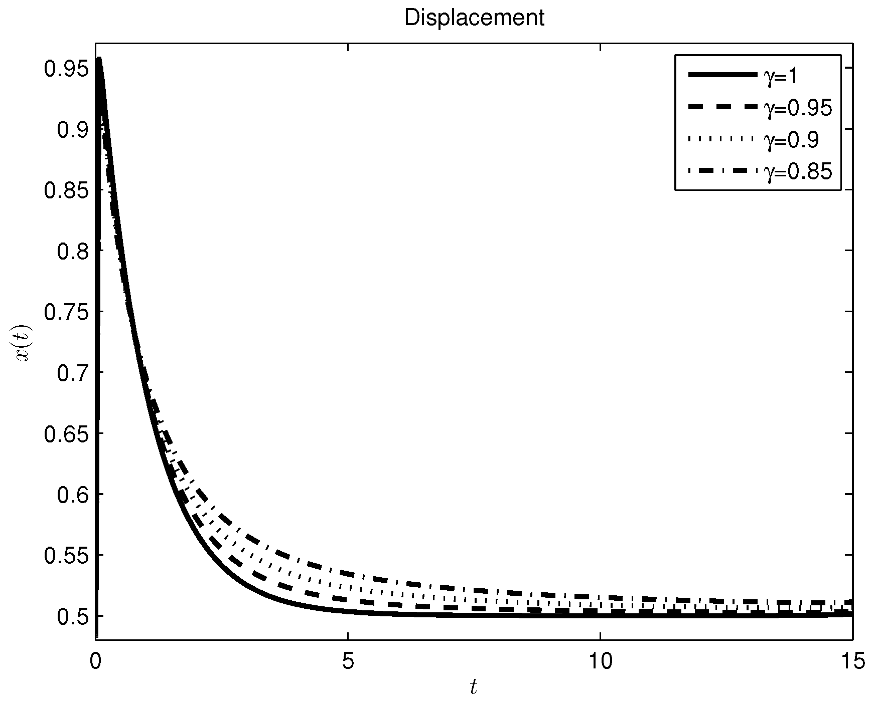
3.1. Mass-Spring System


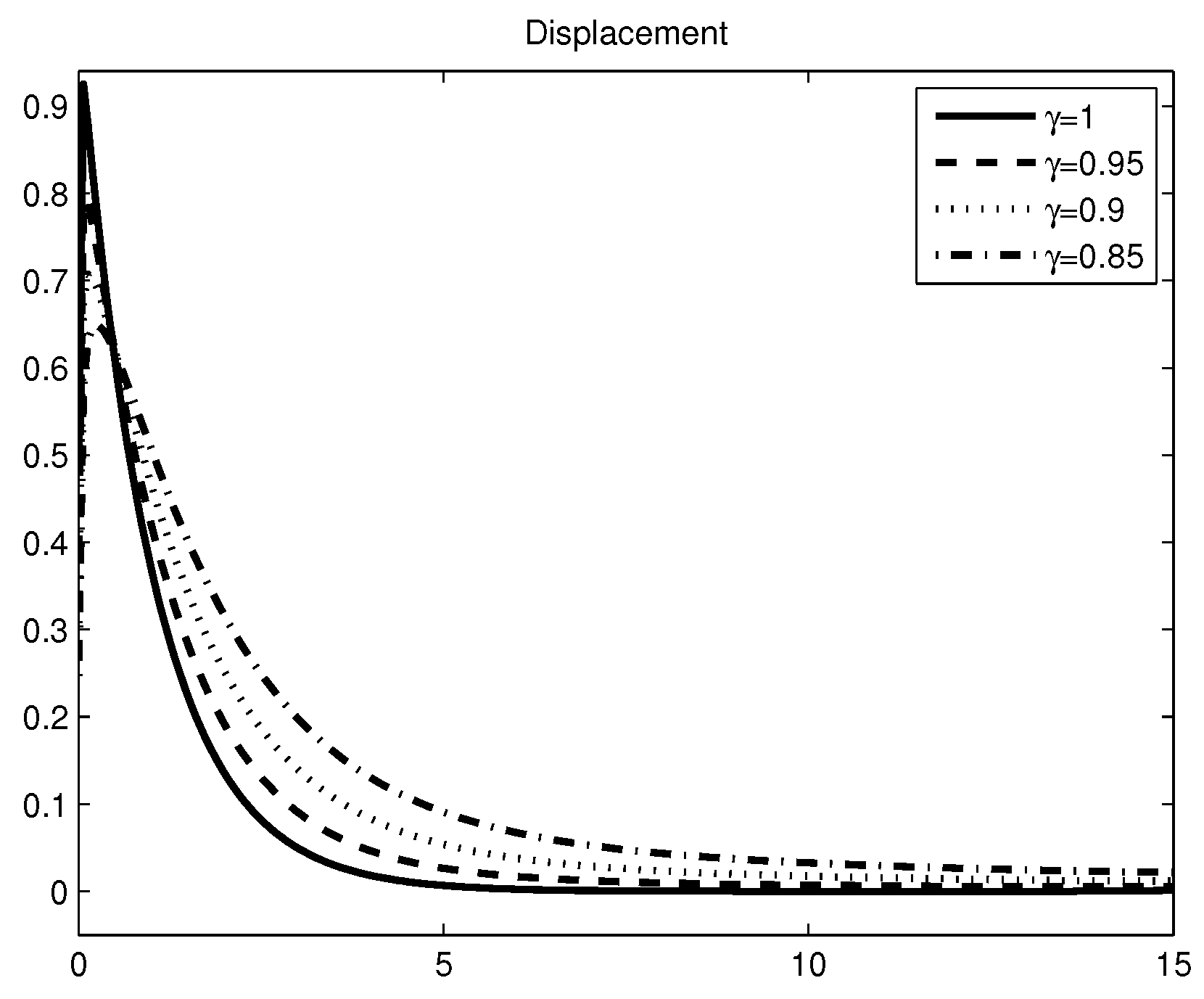
3.2. Damper-Spring System


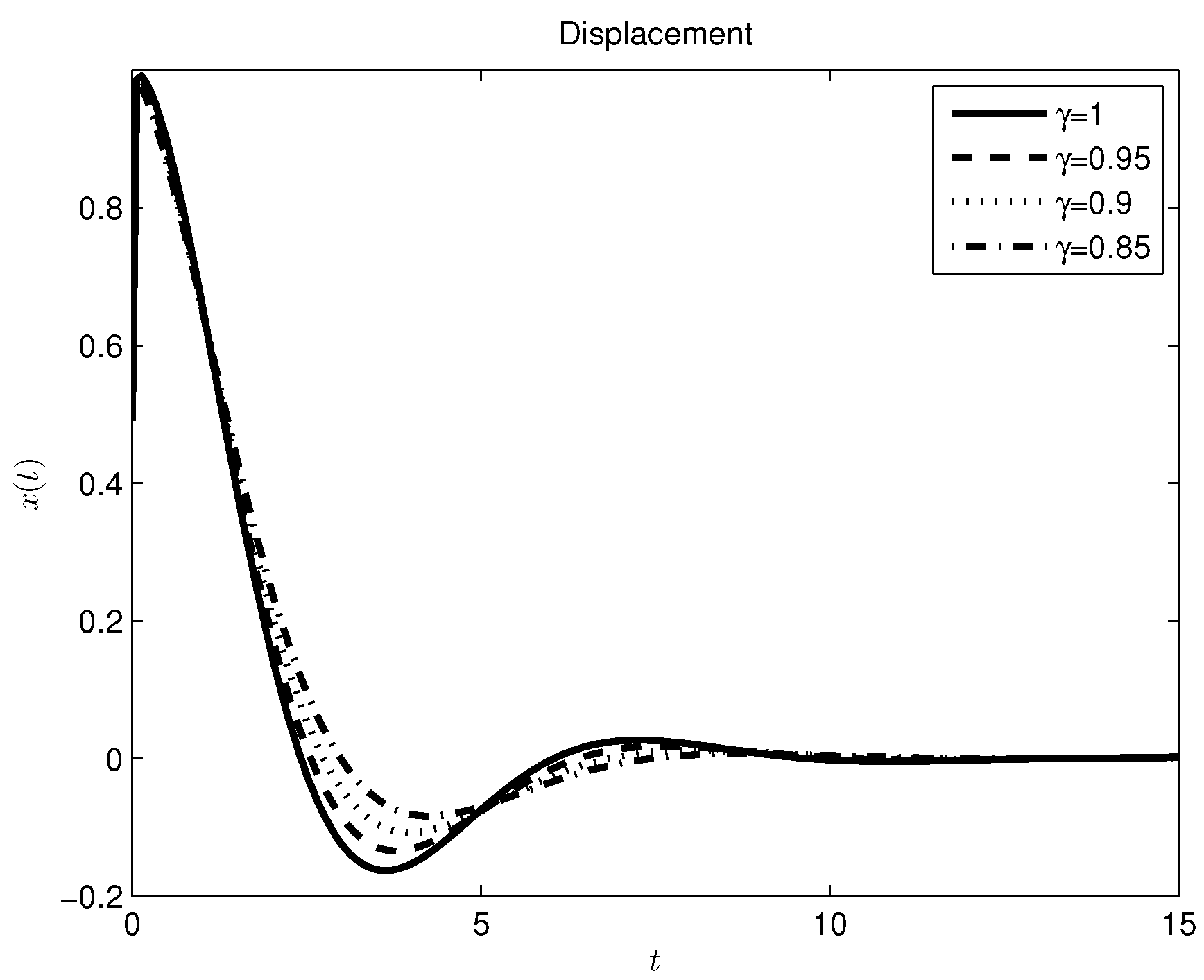
3.3. Mass-Spring-Damper System

4. Conclusion
Acknowledgments
Author Contributions
Conflicts of Interest
References
- Baleanu, D.; Güvenc, Z.B.; Machado, J.A.T. New Trends in Nanotechnology and Fractional Calculus Applications; Springer: Berlin/Heidelberg, Germany, 2010. [Google Scholar]
- Valério, D.; Machado, J.A.T.; Kiryakova, V. Some pioneers of the applications of fractional calculus. Fract. Calc. Appl. Anal. 2014, 17, 552–578. [Google Scholar] [CrossRef]
- Machado, J.A.T.; Kiryakova, V.; Mainardi, F. Recent history of fractional calculus. Commun. Nonlinear Sci. Numer. Simul. 2011, 16, 1140–1153. [Google Scholar] [CrossRef]
- Machado, J.A.T.; Galhano, A.M.; Trujillo, J.J. Science metrics on fractional calculus development since 1966. Fract. Calc. Appl. Anal. 2013, 16, 479–500. [Google Scholar]
- Machado, J.A.T.; Galhano, A.M.S.F.; Trujillo, J.J. On development of fractional calculus during the last fifty years. Scientometrics 2014, 98, 577–582. [Google Scholar] [CrossRef]
- Tarasov, V.E. Fractional Dynamics: Applications of Fractional Calculus to Dynamics of Particles, Fields and Media; Springer: Berlin/Heidelberg, Germany, 2011. [Google Scholar]
- Magin, R.L. Fractional Calculus in Bioengineering; Begell House: Redding, CT, USA, 2006. [Google Scholar]
- Gómez-Aguilar, J.F.; Miranda-Hernández, M. Space-Time fractional diffusion-advection equation with caputo derivative. Abstr. Appl. Anal. 2014, 2014. [Google Scholar] [CrossRef]
- Mainardi, F. An historical perspective on fractional calculus in linear viscoelasticity. Fract. Calc. Appl. Anal. 2012, 15, 712–717. [Google Scholar] [CrossRef]
- Luchko, Y.; Kiryakova, V. The mellin integral transform in fractional calculus. Fract. Calc. Appl. Anal. 2013, 16, 405–430. [Google Scholar] [CrossRef]
- Gómez-Aguilar, J.F.; Miranda-Hernández, M.; López-López, M.G.; Alvarado-Martínez, V.M.; Baleanu, D. Modeling and simulation of the fractional space-time diffusion equation. Commun. Nonlinear Sci. Numer. Simul. 2016, 30, 115–127. [Google Scholar] [CrossRef]
- Machado, J.A.T.; Lopes, A.M. Analysis of natural and artificial phenomena using signal processing and fractional calculus. Fract. Calc. Appl. Anal. 2015, 18, 459–478. [Google Scholar] [CrossRef]
- Kiryakova, V. The multi-index Mittag–Leffler functions as an important class of special functions of fractional calculus. Comput. Math. Appl. 2010, 59, 1885–1895. [Google Scholar] [CrossRef]
- Mishra, V.; Vishal, K.; Das, S.; Ong, S.H. On the solution of the nonlinear fractional diffusion-wave equation with absorption: A homotopy approach. Zeitschrift für Naturforschung A 2014, 69, 135–144. [Google Scholar] [CrossRef]
- Gómez-Aguilar, J.F.; Yépez-Martínez, H.; Escobar-Jiménez, R.F.; Astorga-Zaragoza, C.M.; Morales-Mendoza, L.J.; González-Lee, M. Universal character of the fractional space-time electromagnetic waves in dielectric media. J. Electromagn. Waves Appl. 2015, 29, 727–740. [Google Scholar] [CrossRef]
- Garra, R.; Giusti, A.; Mainardi, F.; Pagnini, G. Fractional relaxation with time-varying coefficient. Fract. Calc. Appl. Anal. 2014, 17, 424–439. [Google Scholar] [CrossRef]
- Gómez-Aguilar, J.F.; Baleanu, D. Solutions of the telegraph equations using a fractional calculus approach. Proc. Romanian Acad. Ser. A 2014, 15, 27–34. [Google Scholar]
- Kiryakova, V. From the hyper-Bessel operators of Dimovski to the generalized fractional calculus. Fract. Calc. Appl. Anal. 2014, 17, 977–1000. [Google Scholar] [CrossRef]
- Gómez-Aguilar, J.F.; Baleanu, D. Fractional transmission line with losses. Zeitschrift für Naturforschung A 2014, 69, 539–546. [Google Scholar] [CrossRef]
- Kutay, M.A.; Ozaktas, H.M. The fractional fourier transform and harmonic oscillation. Nonlinear Dyn. 2002, 29, 157–172. [Google Scholar] [CrossRef]
- Ryabov, Y.E.; Puzenko, A. Damped oscillations in view of the fractional oscillator equation. Phys. Rev. B 2002, 66, 184201. [Google Scholar] [CrossRef]
- Naber, M. Linear fractionally damped oscillator. Int. J. Differ. Equ. 2010, 2010. [Google Scholar] [CrossRef] [PubMed]
- Stanislavsky, A.A. Fractional oscillator. Phys. Rev. E 2004, 70, 051103. [Google Scholar] [CrossRef]
- Tarasov, V.E. The fractional oscillator as an open system. Cent. Eur. J. Phys. 2012, 10, 382–389. [Google Scholar] [CrossRef]
- Caputo, M. The memory damped seismograph. Boll. Geofis. Teor. Appl. 2013, 54, 217–228. [Google Scholar]
- Gómez-Aguilar, J.F.; Rosales-García, J.J.; Bernal-Alvarado, J.J.; Córdova-Fraga, T.; Guzmán-Cabrera, R. Fractional mechanical oscillators. Revisa Mex. Fis. 2012, 58, 348–352. [Google Scholar]
- Tavazoei, M.S. Reduction of oscillations via fractional order pre-filtering. Signal Process. 2015, 107, 407–414. [Google Scholar] [CrossRef]
- Naranjani, Y.; Sardahi, Y.; Chen, Y.Q.; Sun, J.Q. Multi-objective optimization of distributed-order fractional damping. Commun. Nonlinear Sci. Numer. Simul. 2015, 24, 159–168. [Google Scholar] [CrossRef]
- Li, Z.H.; Au, F.T.K. Damage detection of a continuous bridge from response of a moving vehicle. Shock Vib. 2014, 2014. [Google Scholar] [CrossRef]
- Oldham, K.B.; Spanier, J. The Fractional Calculus; Academic Press: Waltham, MA, USA, 1974. [Google Scholar]
- Atangana, A.; Secer, A. A note on fractional order derivatives and table of fractional derivatives of some special functions. Abstr. Appl. Anal. 2013, 2013. [Google Scholar] [CrossRef]
- Baleanu, D.; Diethelm, K.; Scalas, E.; Trujillo, J.J. Fractional Calculus: Models and Numerical Methods; World Scientiffic: Singapore, Singapore, 2012. [Google Scholar]
- Podlubny, I. Fractional Differential Equations; Academic Press: Waltham, MA, USA, 1999. [Google Scholar]
- Diethelm, K. The Analysis of Fractional Differential Equations; Springer: Berlin/Heidelberg, Germany, 2010. [Google Scholar]
- Diethelm, K.; Ford, N.J.; Freed, A.D.; Luchko, Y. Algorithms for the fractional calculus: A selection of numerical methods. Comp. Methods Appl. Mech. Eng. 2005, 194, 743–773. [Google Scholar] [CrossRef]
- Caputo, M.; Fabrizio, M. A new definition of fractional derivative without singular kernel. Progr. Fract. Differ. Appl. 2015, 1, 73–85. [Google Scholar]
- Lozada, J.; Nieto, J.J. Properties of a new fractional derivative without singular kernel. Progr. Fract. Differ. Appl. 2015, 1, 87–92. [Google Scholar]
- Atangana, A.; Alkahtani, B.S.T. Extension of the resistance, inductance, capacitance electrical circuit to fractional derivative without singular kernel. Adv. Mech. Eng. 2015, 7. [Google Scholar] [CrossRef]
- Atangana, A.; Alkahtani, B.S.T. Analysis of the Keller-Segel model with a fractional derivative without singular kernel. Entropy 2015, 17, 4439–4453. [Google Scholar] [CrossRef]
- Gorenflo, R.; Kilbas, A.A.; Mainardi, F.; Rogosin, S.V. Mittag–Leffler Functions, Related Topics and Applications; Springer: Berlin/Heidelberg, Germany, 2014. [Google Scholar]
- Gómez-Aguilar, J.F.; Razo-Hernández, R.; Granados-Lieberman, D. A physical interpretation of fractional calculus in observables terms: analysis of the fractional time constant and the transitory response. Rev. Mex. Fis. 2014, 60, 32–38. [Google Scholar]
- Sheng, H.; Li, Y.; Chen, Y. Application of numerical inverse Laplace transform algorithms in fractional calculus. J. Frankl. Inst. 2011, 348, 315–330. [Google Scholar] [CrossRef]
© 2015 by the authors; licensee MDPI, Basel, Switzerland. This article is an open access article distributed under the terms and conditions of the Creative Commons Attribution license (http://creativecommons.org/licenses/by/4.0/).
Share and Cite
Gómez-Aguilar, J.F.; Yépez-Martínez, H.; Calderón-Ramón, C.; Cruz-Orduña, I.; Escobar-Jiménez, R.F.; Olivares-Peregrino, V.H. Modeling of a Mass-Spring-Damper System by Fractional Derivatives with and without a Singular Kernel. Entropy 2015, 17, 6289-6303. https://doi.org/10.3390/e17096289
Gómez-Aguilar JF, Yépez-Martínez H, Calderón-Ramón C, Cruz-Orduña I, Escobar-Jiménez RF, Olivares-Peregrino VH. Modeling of a Mass-Spring-Damper System by Fractional Derivatives with and without a Singular Kernel. Entropy. 2015; 17(9):6289-6303. https://doi.org/10.3390/e17096289
Chicago/Turabian StyleGómez-Aguilar, José Francisco, Huitzilin Yépez-Martínez, Celia Calderón-Ramón, Ines Cruz-Orduña, Ricardo Fabricio Escobar-Jiménez, and Victor Hugo Olivares-Peregrino. 2015. "Modeling of a Mass-Spring-Damper System by Fractional Derivatives with and without a Singular Kernel" Entropy 17, no. 9: 6289-6303. https://doi.org/10.3390/e17096289
APA StyleGómez-Aguilar, J. F., Yépez-Martínez, H., Calderón-Ramón, C., Cruz-Orduña, I., Escobar-Jiménez, R. F., & Olivares-Peregrino, V. H. (2015). Modeling of a Mass-Spring-Damper System by Fractional Derivatives with and without a Singular Kernel. Entropy, 17(9), 6289-6303. https://doi.org/10.3390/e17096289