Abstract
This paper examines modern economic growth according to the multidimensional scaling (MDS) method and state space portrait (SSP) analysis. Electing GDP per capita as the main indicator for economic growth and prosperity, the long-run perspective from 1870 to 2010 identifies the main similarities among 34 world partners’ modern economic growth and exemplifies the historical waving mechanics of the largest world economy, the USA. MDS reveals two main clusters among the European countries and their old offshore territories, and SSP identifies the Great Depression as a mild challenge to the American global performance, when compared to the Second World War and the 2008 crisis.
1. Introduction
The decades from the 1870s to the First World War reaped the tremendous benefits of the technological sweep in sectors such as textiles, metallurgy, railways, steam shipping, chemistry and communications. Technological improvements in the inter-war period included the revolutionizing development of electricity, the automobile and flight. After the Second World War, prosperity boomed, making possible consumption that “was difficult for our great-grandparents to imagine. These include an array of advances in information technology—computer-assisted machinery and robots, the Internet, many new communication technologies—as well as breakthrough drugs and medical technologies, improved indoor plumbing, refrigerators and other household durables, better and less expensive lighting, radio, television, inexpensive air and ground travel, and a huge increase in entertainment and culinary options” []. Thanks to the cumulative aspects of technological and organizational improvements, increased production of goods and services has translated into sustainable, unrelenting and uneven economic growth.
This paper assesses the spread of the modern economic growth experience among European countries and the offshore regions that were under European political control as a result of colonization. Will it be possible to identify broad similarities among nations in considering the whole historical process that comes from the 1870s to now?
Different models have been proposed to describe economic systems [,,,]. However, presently, there is no model that describes accurately long-term dynamics, reflecting not only economical, social, political, ethnically, religious and cultural aspects, but also emerging topics, such as global warming and natural catastrophic events. Instead of using explicit models, we explore economic data in the perspective of dynamical systems. We consider that the GDP per capita of each country is a state variable of a set of multiple possibly coupled dynamic subsystems. Long time series are considered so that memory effects can emerge. For studying the dynamics, we apply two distinct methodologies, namely multidimensional scaling (MDS) and space state portrait (SSP). MDS is a technique for visualizing information in data. SSP represents the sequence of points corresponding to the system states over time. We generalize the SSP using the tools of fractional calculus (FC), and we introduce the novel concept of fractional state space portrait (fSSP). FC has been successfully applied in many phenomena with long-memory, but in the area of economy, it has been mainly oriented toward statistical effects. Several proposals for the interpretation of fractional derivatives can be found in the literature [,]; nevertheless, the topic is still far from being stabilized.
Optimistic and pessimistic views refer to economic convergence versus divergence, respectively, as Section 2 records. This is as a major issue for humankind, of course []. MDS methodologies can contribute to this debate in a decisive way, in assessing similarities and dissimilarities of the major indicator for average prosperity and welfare, the GDP per capita. The colonized regions for which it is possible to collect yearly data show an uneven growth, which means that sizeable gaps still exist among nations []. In fact, two different clusters of nations are identified, one made of less-developed countries that sprang from decolonization. However, the presence of earlier colonial nations in the cluster of the most developed countries of the world is optimistic evidence about the spread of the modern economic growth experience. They are real outliers of the pessimistic view. Along with the USA, the examples in the sample studied also include Canada, Brazil and Colombia. These countries’ GDP per capita performances have replicated the most developed countries process of modernization, and the MDS methodology simply confirms the current expectations for their future highly-developed status in the world.
Whatever the analysis one may perform on the period from the 1870s until today, the great global economic growth winner has been the American economy []. Victorious in both world wars, the American economic growth from the end of the American civil war to now has conferred a decisive role to the USA’s performance in the world, in terms of geopolitics [].
In spite of globalization and the resulting integration of markets in an international perspective, the USA has revealed a capacity to weather through crises. It is argued that “the United States has been comparatively immune to crises” (citing especially the performance of equity returns and stock markets []). Accepting this perspective means that it is appropriate to look at the global economic growth in considering the performance of the American economy []. SSP may be useful in describing loops that are characteristic of crises.
Unemployment, social problems, globalization and crises synchronization have become a concern in the new millennium (business cycles are becoming more synchronized []). Given the economically weak international environment, the global financial crisis also “may have caused European business cycles to become more strongly synchronized” []. In such a context, what is the meaning of crises in the American economy? How can nineteenth-century economic volatility compare to the Great Depression, the two World Wars problems, the 1980s, the late 1990s and the 2008 financial crisis?
The SSP methodology reveals how much more overwhelming America’s Second World War effort was for its economy than the 1929–1933 crisis, which, however, has earned the label of the Great Depression. Although data on the 2008 crisis are incomplete, our SSP analysis also points to the high severity of this recent challenge for the dominant global economy. As a leading power, America’s economic fluctuations surely impact other countries’ economic growth and volatility []. The study of the American economic growth may also be the study of the Western world’s economic growth, a subject to be appraised in future research.
The quality of data requires the selection of appropriate historical samples for GDP time series. Of course “Economic historians worry (...) about the reliability of the historical series, but accept the output of countries’ statistical offices at face value” []. Section 2 will present literature perspectives. Section 3 describes the data used, and Section 4 and Section 5 present the MDS and the SSP methodologies and their estimates. Results are interpreted as conclusions.
2. Literature Review
The effects of colonization on the economic growth of colonized regions have been widely discussed. As this is a political subject, the discussion has given way to early contributions on exploitation and imperialism theses [], with recent interpretations stressing the importance of the correlation between institutional gaps derived from colonialism and under development []. Colonization seems to be one of the long-run determinants of economic growth and prosperity. Tropical climate and diseases seem to have been less decisive for under development than the negative effects of the European colonization on the organizational features of colonized offshores. A reversal of fortune even occurred after the beginning of colonization in 1500 in many regions, due to institutional features []. Forced labor (slavery) inflicted negative effects on the population distribution of societies where extractive institutions could perform. The conditions for industrialization became quite asymmetrical where European plantation systems produced large interests and profits for European countries. The Portuguese and Spanish colonization systems have been presented as cases of high concentration of political power in the hands of a few who extracted resources from the rest of the population to obtain gold, silver and other valuables from America. The monopoly of the political power was at the service of plantation systems and mining []. Only when Europeans introduced institutions more favorable to private property ownership in regions that were sparsely populated could colonization be less negative, particularly because Europeans could settle there in large numbers []. As settled Europeans were also affected by these institutions, they developed institutions to frame effective property rights, as in the USA and Canada, for example.
The volatility of modern economic growth has also been a subject deserving historians’ attention with the purpose of comparing the 2008 challenges with previous financial crises. Barry Eichengreen’s and O’Rourke’s comparison between the Great Depression and the 2008 crisis is based on world indicators and does not address the USA case []. Shachmurove [] identifies 1857, 1873 and 1893 as American crises provoking widespread panic, and cites 1907, 1929–1933 and the 2008 financial crisis as the main twentieth-century financial busts. Claiming that “these financial crises are similar in their nature”, there is no reference to the Second World War GDP challenges, and the restricted analysis that is made does not allow a long-run comparison for the GDP per capita fluctuations. The conclusion is that future crises will be difficult, indeed impossible, to eliminate. Tallman [] compares the 1907 and 2008 crises to conclude that “for the most part these financial crises are similar in their nature”, but does not assess their relative dimension.
3. Data and Methodology
Data were collected from the Maddison Project [,], available on the website http://www.ggdc.net/ maddison/maddison-project/home.htm. The goal of the project is to establish an inventory of historical national accounts. The dataset info-indicator is the GDP per capita of the world during the years 0001 up to 2010, with units of 1990 GK dollars per capita. However, the dataset has very limited information for early years. Therefore, we established a compromise between having a large number of countries and having assertive data. We selected the period 1870–2010 for countries, namely Argentina, Australia, Austria, Belgium, Brazil, Canada, Chile, Colombia, Denmark, Ecuador, Finland, France, Germany, Greece, India, Italy, Japan, Mexico, the Netherlands, New Zealand, Norway, Peru, Portugal, Romania, South Africa, Spain, Sri Lanka, Sweden, Switzerland, Turkey, Uruguay, Venezuela, the U.K. and the USA. Still, for Argentina, Ecuador, India, Mexico, Romania, South Africa and Turkey, some small periods were lacking information that was completed by interpolating between adjacent years.
Data are interpreted as one manifestation of a complex system of dynamic evolution over time. We consider that the GDP per capita of country i (), to be denoted by , is a state variable of a set of n possibly coupled dynamic subsystems, where t represents time. Two approaches are possible for studying the dynamics: either to develop some kind of analytic model or to analyze real data by means of computational and numerical tools.
In this paper, we follow the second direction by applying two distinct methodologies for visualizing system behavior, namely MDS and SSP.
4. MDS Analysis of World Economies
MDS is a technique for visualizing information in data [,,,,,,]. MDS was successfully applied to economy dynamics [,] and requires the definition of a similarity index and the construction of an matrix C of item-to-item similarities, where n is the total number of items in an r-dimensional space. In classic MDS, C is symmetric and its main diagonal is composed of “1”. Based on that information, MDS extrapolates an approximate map in a u-dimensional space () with the objects’ locations. MDS uses a function minimization algorithm that evaluates different configurations with the goal of maximizing a goodness-of-fit. By rearranging the items, positions in the u-space, MDS arrives at a configuration that best approximates the reproduced and observed similarities. For low dimensional spaces (e.g., or ), the resulting points can be displayed in a map. The MDS interpretation is based on the emerging clusters and distances between points in the map, rather than on their absolute coordinates or the geometric form of the locus. We can rotate or translate the MDS map since the distances between points remain identical.
Stress and Shepard plots are standard tools for assessing the MDS results. The stress plot represents the goodness-of-fit function versus the number of dimensions u of the MDS map, leading to a monotonic decreasing chart. The user chooses the “best” dimension u as a compromise between stress reduction and number of dimensions. The Shepard diagram compares the reproduced to the observed similarities. Therefore, a narrow/large scatter around a 45-degree line indicates a good/bad fit.
In Section 4.1 and Section 4.2, we adopt the Pearson correlation and the mutual information as similarity indexes, and we use MDS for comparing the GDP per capita time series.
4.1. MDS Analysis Based on the Pearson Correlation
Here, we construct the matrix , dimensional, based on the Pearson correlation between the GDP per capita time series of country pairs , i.e., and , respectively:
where P denotes the length of the time series and represents the arithmetic mean.
The MDS maps for and are depicted in Figure 1, where each point represents a country. A shorter (larger) distance between two points on the maps means that the corresponding objects are more (less) similar.
We can see that the countries are organized into two main clusters according to . Cluster Argentina, Chile, Ecuador, India, Mexico, Peru, South Africa, Sri Lanka, Uruguay, Venezuela} includes less developed countries, while Australia, Austria, Belgium, Brazil, Canada, Colombia, Denmark, Finland, France, Germany, Greece, Italy, Japan, the Netherlands, New Zealand, Norway, Portugal, Romania, Spain, Sweden, Switzerland, Turkey, the U.K., the USA} includes the most developed economies plus Brazil and Colombia.
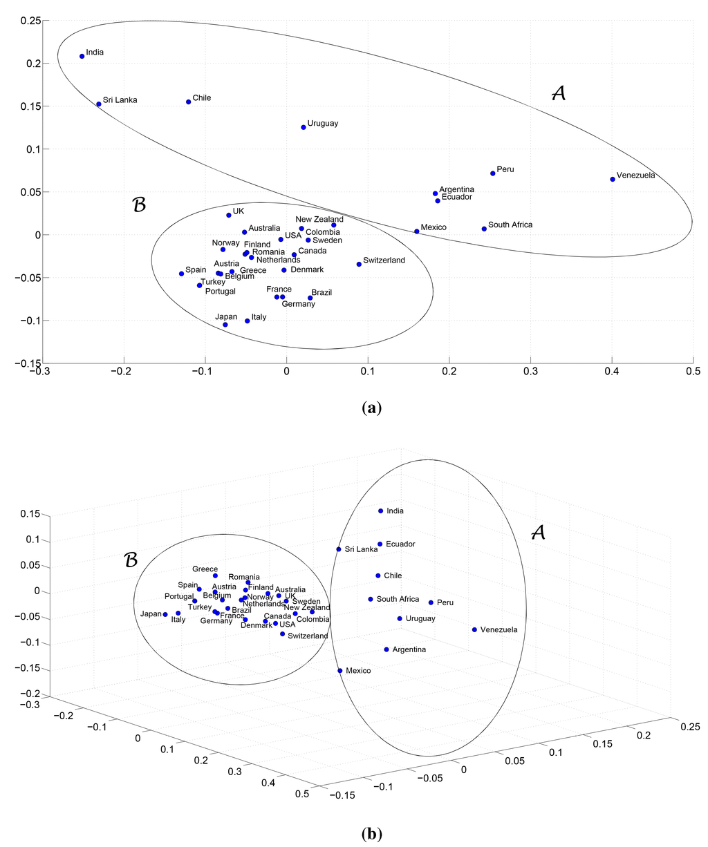
Figure 1.
The multidimensional scaling (MDS) maps for the Pearson correlation between the GDP per capita time series 1870–2010 of n = 34 countries: (a) two-dimensional; (b) three-dimensional.
Figure 2 and Figure 3 depict the Shepard and stress plots, respectively. The Shepard diagram shows a good distribution of points around the 45-degree line, particularly for , which means a good fit of the reproduced similarities into the observed similarities. The stress plot reveals that a three-dimensional space describes well the locus of the countries. In fact, the stress diminishes strongly until the dimensionality is two, moderately toward dimensionality three and weakly from then on. The maximum curvature point of the stress plot is often adopted as the criterion for deciding the dimensionality of the MDS maps. This means that although four or more dimensions would represent the data more accurately, three-dimensional maps are a good compromise between accuracy and ease of visualization.
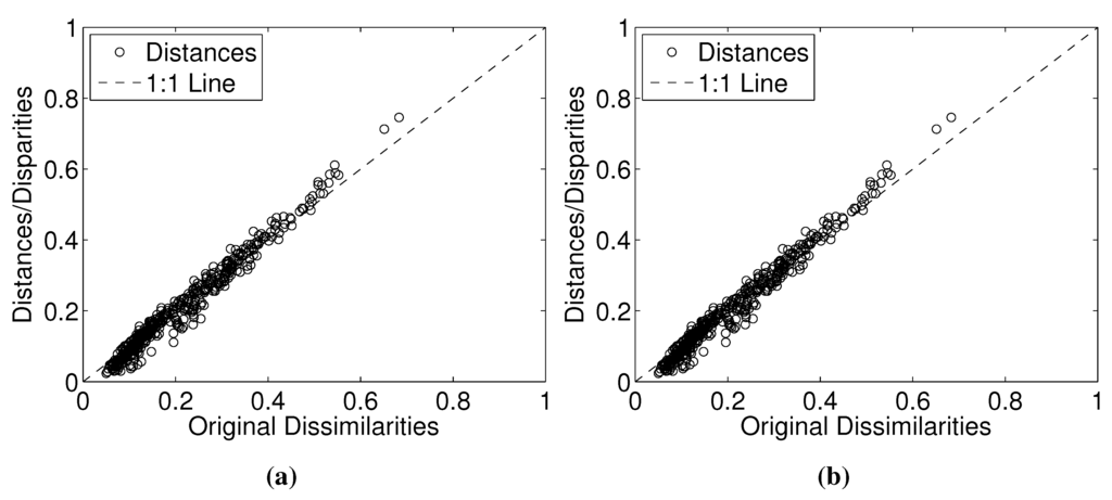
Figure 2.
Shepard plots for the Pearson correlation between the GDP per capita time series 1870–2010 of n = 34 countries for representations: (a) two-dimensional; (b) three-dimensional.
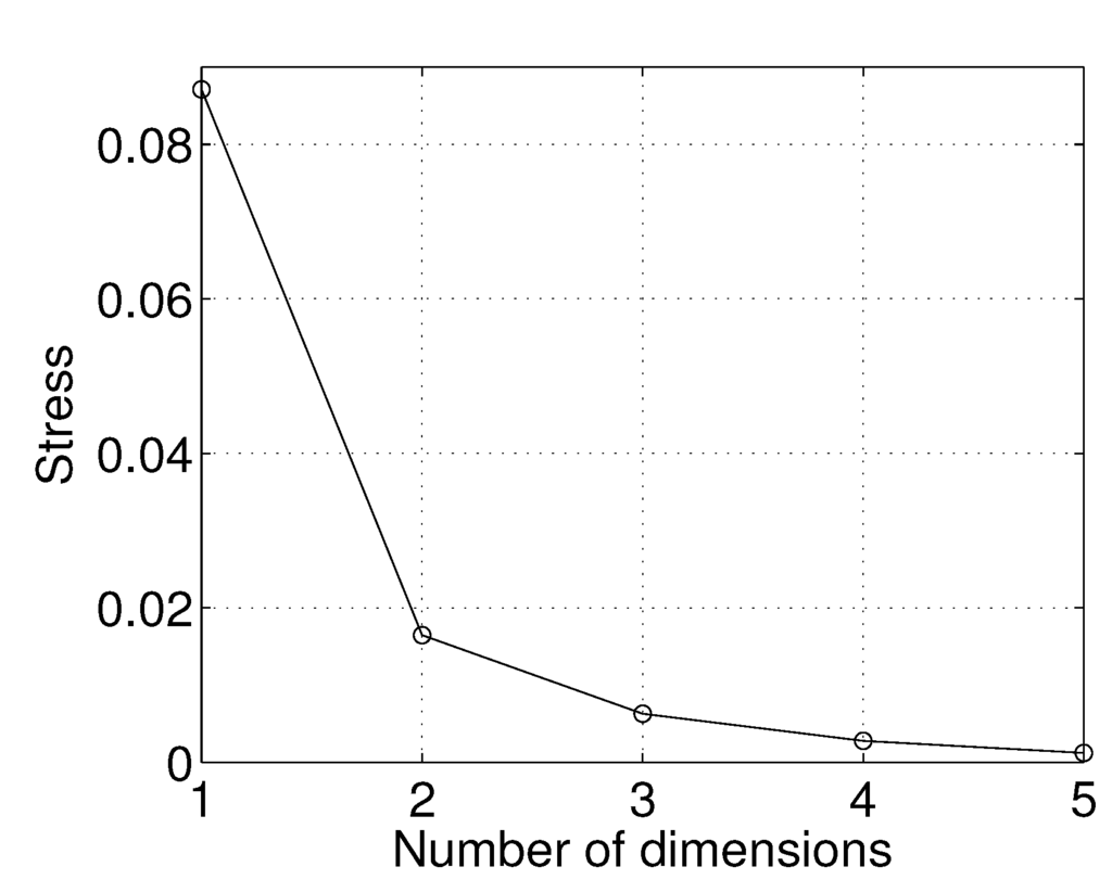
Figure 3.
Stress plot for the Pearson correlation between the GDP per capita time series 1870–2010 of countries.
4.2. MDS Analysis Based on the Mutual Information
The mutual information has been introduced in the context of information theory and then adopted as a common approach to the analysis of complex systems [,]. Mutual information measures the statistical dependence between two random variables, yielding the amount of information that one variable “contains” about the other. Mathematically, for the discrete random variables , the mutual information, is given by:
where and represent the marginal probability distribution functions of X and Y, respectively, and is the joint probability distribution function. The mutual information is always nonnegative and symmetric, meaning that .
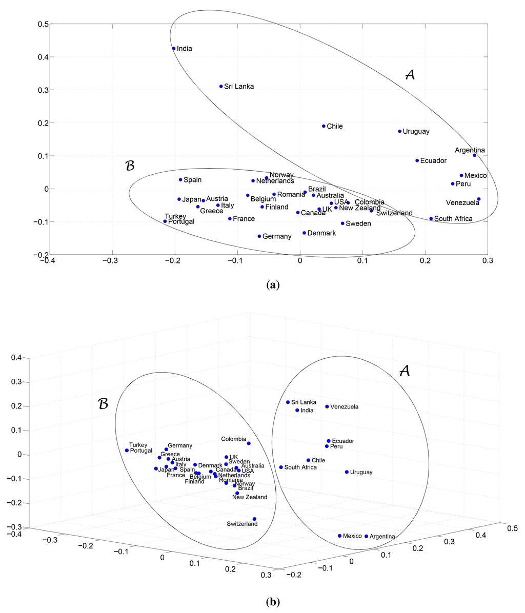
Figure 4.
The MDS maps for the normalized mutual information between the GDP per capita time series 1870–2010 of n = 34 countries: (a) two-dimensional; (b) three-dimensional.
Often the normalized mutual information, , is adopted []:
with representing the entropy:
In this case, , for . The normalized mutual information has the advantage of simplifying comparison across different conditions and improving sensitivity.
Using Equation (3), the similarity matrix is now given by , where represents the normalized mutual information between the GDP per capita time series of country pairs . The probabilities were estimated by means of the histograms of relative frequencies.
The MDS maps for and are depicted in Figure 4, where we can see the emergence of the same clusters already identified in Section 4.1. Moreover, the Shepard and stress plots corresponding to the 2- and 3-dimensional MDS maps are similar to the those shown in Figure 2 and Figure 3.
We tested additional indices, besides (1) and (3), namely the cosine, the Kendall and the Spearman correlations. All of these indices yield identical results, leading to the conclusion that the MDS approach is robust from the perspective of the index to be adopted.
5. State Space Analysis of World Economies
A k-dimensional dynamic system can be represented by a set of first-order differential equations governing k state variables, . Such equations are obtained from the system input-output functional relationship (i.e., system model), for a given set of state variables. Knowing at time and the system inputs for , we can determine the system behavior for . The state space consists of the set of all possible states, each one corresponding to a unique point. As t evolves, we obtain sequences of points describing trajectories in the state space. The set of trajectories is the SSP. For first-, second- and third-order systems, the SSP can be depicted on a map, and the system behavior can be inferred from the corresponding graphic representation [].
In this section, we study the GDP per capita time series by means of SSP. In Section 5.1, we adopt the classic formulation based on integer-order time derivatives. In Section 5.2, we use the tools of FC and propose a generalization that leads to the concept of fSSP.
5.1. Classic State Space Portrait
For constructing the SSP, we can use the time series and its integer-order time derivatives, often called phase variables. The adoption of a k-dimensional representation is a compromise between assertiveness and feasibility. As the order of a hypothetical differential model is unknown, we need to test successive increasing orders of the state space representation. On the other hand, the selection of the state variables poses problems, since some common economy indices may fail to assertively reflect the state dynamics or may not be independent of each other. The adoption of phase variables (i.e., the time derivatives) is somewhat abstract, but assures a solid formulation.
The numerical calculation of the integer-order derivatives needs a careful design of the algorithm, since noise may occur, saturating the resulting signal. We adopt the algorithm proposed in []:
where h denotes the sampling period.
We must observe that Equation (5) requires two additional points at the left and right. Therefore, the SSP turns out to be limited to the period 1872–2008, making a total of data points. Several numerical experiments demonstrated that these formulae produce good results for the time series under analysis.
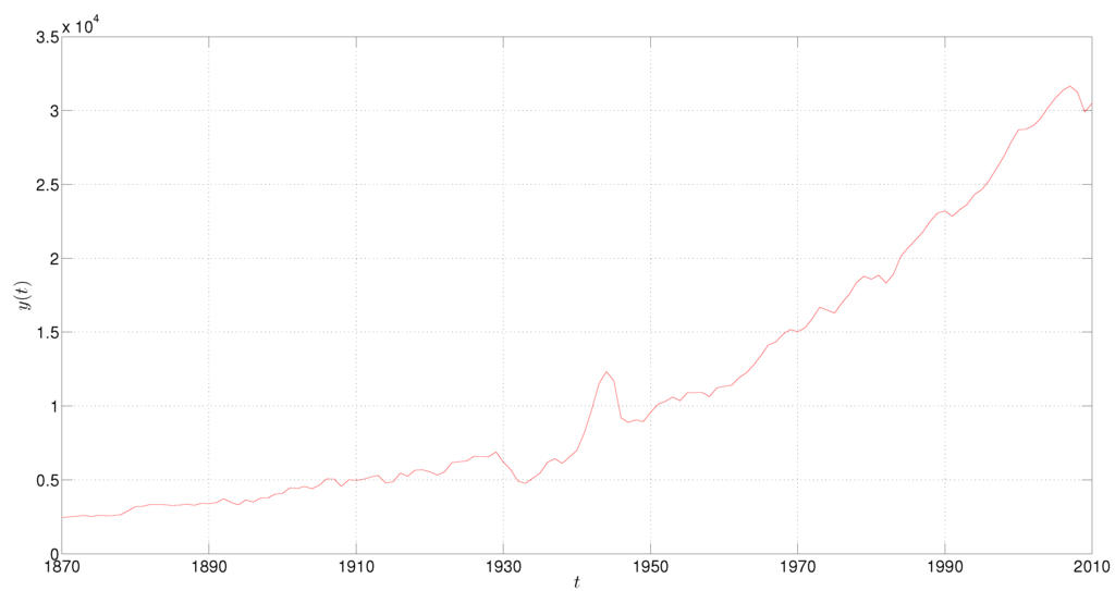
Figure 5.
The GDP per capita of the USA during 1870–2010.
For example, Figure 5 and Figure 6 show the time evolution of the USA’s GDP per capita and the corresponding two- and three-dimensional representations in the phase space, with year. The “main loops” correspond to historical periods of economic fluctuations. Economic growth went on at a long-run increasing rate []. The 1929–1933 crisis has become the benchmark of financial crises []. The 1929 New York Stock Exchange crash, the scarce demand for commodities, the tremendous consequences on production units, the reduction of employment (thanks to part-time options and lay-outs), the social problems of jobless people, the contagious effects to other countries and the collapse of international trade were the hallmarks of the lengthy depression [,]. The recovery brought a rapid economic growth rate that lasted until the effects of the Second World War on the American economy, thanks to good opportunities for many economic sectors. However, the participation of the USA in the war had consequences on the growth rate, which were overcome with the Bretton Woods monetary regime and the prosperity of the next decades []. The consequences of the dollar flood and Vietnam War on the declaration of the dollar inconvertibility in 1971 brought more volatility to the American economy, particularly in the context of the oil shock of 1973 (and the 1979 second shock, in the context of the Iranian revolution of 1978–1979) []. The dot-com recession of the early 2000s and the 2008 financial crisis also deserve to be mentioned.
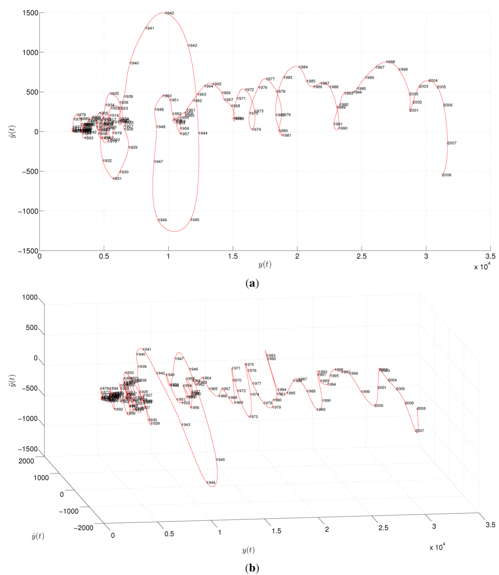
Figure 6.
The state space portrait (SSP) for the USA GDP per capita time series 1872–2008: (a) two-dimensional map; (b) three-dimensional map.
We observe that the two-dimensional locus reveals some overlapping of the trajectories that are absent in the three-dimensional SSP. Experiments with other countries produce the same types of results. Therefore, we conclude experimentally that the three-dimensional locus overcomes the non-uniqueness trajectory problem visible in lower dimensions. Nevertheless, when using integer-order derivatives, we are limited in our options, since for , the SSP is difficult to represent and to interpret.
5.2. Fractional-Order State Space
We propose generalizing the SSP approach by using the tools of FC. This generalization leads to a “more efficient” representation of the system dynamics, since we are not limited to integer-order derivatives. Therefore, for a given k-dimensional space, we have a broader set of options for the SSP.
The methodology is as follows. In the first step, we determine the order of the derivatives that lead to the better fSSP representation of the i-th country. Second, we adopt the order of the derivatives as a signature of each subsystem behavior, and we analyze the relationships between them. Third, the results are compared to those obtained with MDS, revealing the feasibility of the proposed approach for visualizing system dynamics.
FC extends the concepts of derivative and integral to non-integer orders. During recent decades, FC has been found to play a fundamental role in modeling many important physical phenomena and has emerged as an important tool in the area of dynamic systems with complex behavior [,,,,,,,,,,,,,].
Several definitions of fractional derivative and integral have been proposed [,,]. We recall here the Grünwald–Letnikov (GL) fractional “differintegral” operator of order , , given by []:
where denotes the integer part operator, h is the time increment and , are the upper and lower limits of the “differintegral” operation, respectively.
Due to the summation form of the GL definition, the fractional-order derivative can easily implemented numerically in a computer []. This is usual in numerical methods, in signal processing and in control. Other formulations, such as Riemann–Liouville and Caputo, are often used in mathematics, physics and more abstract research [,].
Equation (6) is approximated by [,]:
where T is the sampling period, L corresponds to the “memory length” and .
The binomial coefficients are given by []:
Parameter L can be chosen using the criterion:
where is the maximum admissible normalized error, given by:
For determining the order of the time derivatives for the fSSP of the i-th country, we compare s fractional-order derivatives , with α evenly distributed in the interval . In Section 5.2.1 and Section 5.2.2, we adopt the Pearson correlation and the mutual information as comparison indexes.
5.2.1. Determination of the fSSP Based on the Pearson Correlation
For the i-th country, we calculate the Pearson correlation, , between each derivative pair , .
Figure 7 depicts the contour maps of obtained for the USA GDP per capita. All countries yield similar results. We focus on the isocline that contains the point , i.e., the point corresponding to the zero- and first-order derivatives, respectively, since this is the classic (integer-order) approach. We observe that the value is obtained for different pairs . The point of maximum isocline curvature is a trade-off between derivative orders. Closer to the left-end point of the isocline, we see that is more sensitive to , while closer to the right-end point of the isocline, it is more sensitive to . At point , the index depends equally on , establishing a good compromise between both variables and yielding the two-dimensional fSSP of Figure 8. As for the SSP, the “main loops” correspond to historical periods of economic fluctuations.
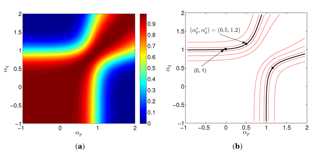
Figure 7.
Maps of for the GDP per capita of USA during 1870–2010: (a) contour plot; (b) contour plot showing a few isoclines.
It should be noted that with the fSSP, we have many alternatives for visualizing the system dynamics, even in two dimensions, opening the possibility of obtaining a good representation in low dimensional spaces. Therefore, other schemes can be explored in the future to obtain the values of fractional orders.
We applied this methodology to the GDP per capita time series of all countries, leading to charts of the same type as the one in Figure 7.
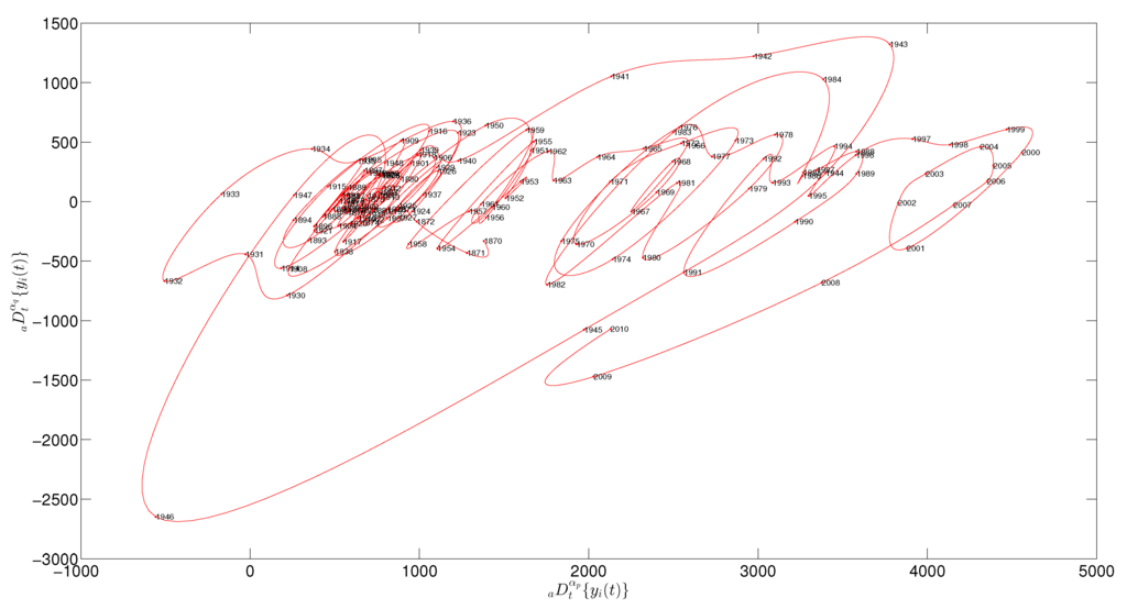
Figure 8.
The two-dimensional SSP for the GDP per capita of the USA during 1870–2010.
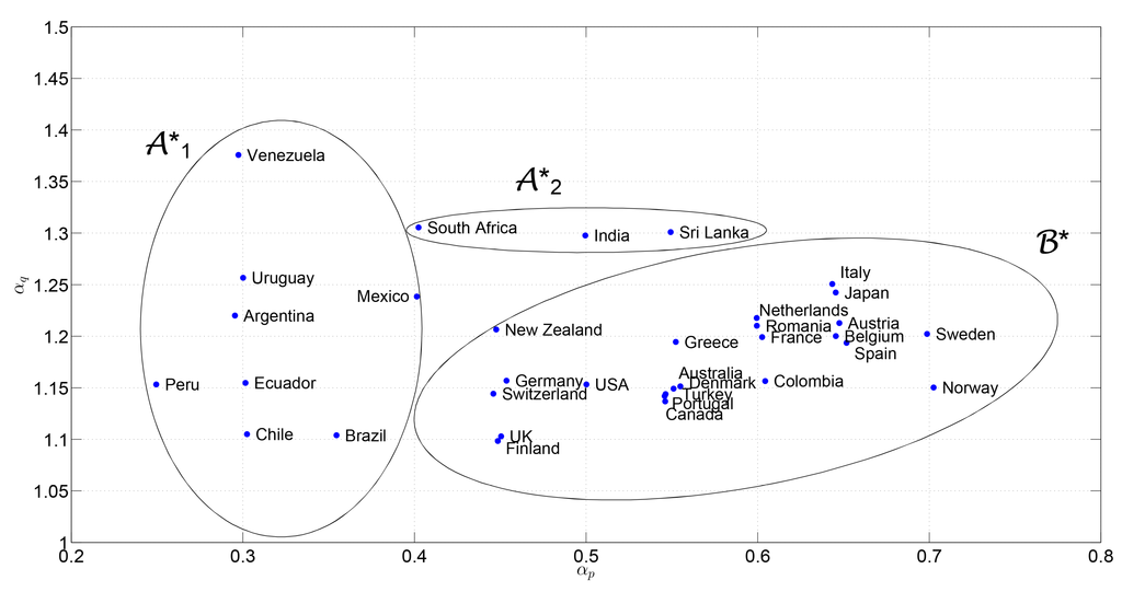
Figure 9.
Locus of points corresponding to the maximum curvatures of the isoclines that contain the point , obtained with the Pearson correlation.
Figure 9 represents the locus of pairs for the set of countries obtained as described above. Each point is interpreted as a dynamic characterization of each country. We can see that the countries fall into two main clusters according to : and . Furthermore, for subcluster Argentina, Brazil, Chile, Ecuador, Peru, Uruguay, Venezuela}, we observe that the countries are characterized essentially by , while remains almost the same. For subcluster India, South Africa, Sri Lanka}, we have a strong dependence on , while remains constant. For cluster Austria, Australia, Belgium, Canada, Colombia, Denmark, Finland, France, Germany, Greece, Italy, Japan, the Netherlands, the U.K., Switzerland, the USA, New Zealand, Norway, Portugal, Romania, Spain, Sweden, Turkey}, we verify a strong dependence on both and .
Clusters and are identical to those identified by the MDS and shown in Figure 1 (with the exception of Brazil). However, with the emergence of the subclusters and , we can conclude that the methodology based on the fSSP is better for discriminating among countries.
5.2.2. Determination of the fSSP Based on the Mutual Information
For each country, we now calculate the normalized mutual information, , between the derivative pairs , .
Figure 10 depicts the contour map of obtained for the USA GDP per capita. When compared to Figure 7a, we see a similar chart (but with more “noise”). All countries yield identical results.
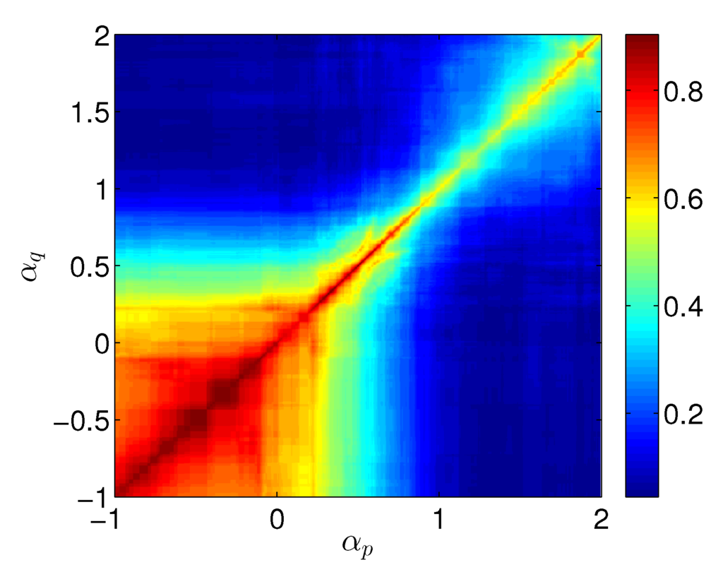
Figure 10.
Contour plot of for the GDP per capita of the USA during 1870–2010.
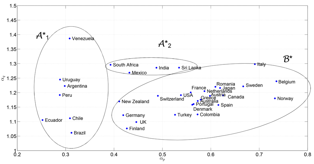
Figure 11.
Locus of points corresponding to the maximum curvatures of the isoclines that contain the point , obtained with the mutual information, .
Figure 11 represents the locus of pairs , where we see the emergence of the same clusters identified in Figure 9, with the exception of Mexico, which leaves cluster towards .
We tested different indices, besides the Pearson correlation and the mutual information, namely the cosine, the Kendall and the Spearman correlations. Those indices produced the same type of results. Therefore, we conclude that the approach is robust regarding the index chosen for calculating the order of the time derivatives for the fSSP.
6. Conclusions
The MDS methodology that was applied to a sample of 34 countries points to the conclusion that two different clusters of countries may be identified in the long-run process of modernization that has occurred from 1870–2010. Confirming the literature, one of the clusters comprises partners that emerged from decolonization, and their path is quite different from the one of European colonizers. However, four countries among the 34 analyzed also emerged from decolonization, but present strong similarities to the European colonizers regarding the whole process of economic growth and industrialization. The fact that they were subject to colonization has not been a handicap for modern economic growth. Brazil, Canada, Colombia and the USA are the four countries that are real outliers. Curiously, in applying SSP methodologies, three clusters become visible. Brazil moves from the European to the colonized-countries’ cluster, and India, Mexico, South Africa and Sri Lanka move to a midway position between the European and the other-colonized partners’ cluster. The historical evidence associated with the methodologies used does not allow for the formulation of a general conclusion on the negative consequences of colonization. Moreover, if the success of the USA and Canada may praise the British and French colonization systems of settlement, Brazil and Colombia do not confirm the extractive character of the Portuguese and Spanish colonization systems. The fractional-order SSP for the USA’s GDP per capita reveals that the major challenge to the USA’s economy was the Second World War conflict, and the 2008 crisis recovery has prevented a severity of duress comparable to that of WWII. Because of the large size and global dominance of the economy of the USA, the Figure 7 SSP analysis brings some confidence about the world recovery, confirming Eichengreen and O’Rourke’s perspective.
Acknowledgments
We thank John Huffstot for correcting our English.
Author Contributions
J. A. Tenreiro Machado and António M. Lopes conceived and designed the experiments. J. A. Tenreiro Machado and António M. Lopes performed the experiments. J. A. Tenreiro Machado, Maria Eugénia Mata and António M. Lopes analyzed the data. J. A. Tenreiro Machado, Maria Eugénia Mata and António M. Lopes wrote the paper. All authors have read and approved the final manuscript.
Conflicts of Interest
The authors declare no conflict of interest.
References
- Acemoglu, D. The World Our Grandchildren Will Inherit: The Rights Revolution and Beyond; Technical Report; National Bureau of Economic Research: Cambridge, MA, USA, 2012. [Google Scholar]
- Matsumoto, A.; Szidarovszky, F. Nonlinear multiplier–accelerator model with investment and consumption delays. Struct. Chang. Econ. Dyn. 2015, 33, 1–9. [Google Scholar] [CrossRef]
- Dassios, I.K.; Zimbidis, A.A.; Kontzalis, C.P. The Delay Effect in a Stochastic Multiplier–Accelerator Model. J. Econ. Struct. 2014, 3. [Google Scholar] [CrossRef]
- Holcombe, R.G. Economic Models and Methodology; Greenwood Press: Santa Barbara, CA, USA, 1989. [Google Scholar]
- Reiter, M. The Dynamics of Business Cycles: Stylized Facts, Economic Theory, Econometric Methodology and Applications; Springer: Berlin/Heidelberg, Germany, 2012. [Google Scholar]
- Machado, J.T. A probabilistic interpretation of the fractional-order differentiation. Fract. Calc. Appl. Anal. 2003, 6, 73–80. [Google Scholar]
- Machado, J.T. Fractional derivatives: Probability interpretation and frequency response of rational approximations. Commun. Nonlinear Sci. Numer. Simul. 2009, 14, 3492–3497. [Google Scholar] [CrossRef]
- Maddison, A. A Revised Estimate of Italian Economic Growth 1861–1989. PSL Q. Rev. 1991, 44, 225–241. [Google Scholar]
- Maddison, A. Monitoring the World Economy, 1820–1992; Development Centre of the Organisation for Economic Co-operation and Development: Paris, France, 1995. [Google Scholar]
- Maddison, A. Statistics on world population, GDP and per capita GDP; Technical Report; University of Groningen: Groningen, The Netherlands, 2010. [Google Scholar]
- Maddison, A. Phases of Capitalist Development; Oxford University Press: New York, NY, USA, 1982. [Google Scholar]
- Barro, R.J.; Ursúa, J.F. Macroeconomic Crises since 1870; NBER working-paper no. 13940; National Bureau of Economic Research: Cambridge, MA, USA, 2008. [Google Scholar]
- Allen, W.A.; Moessner, R. The international propagation of the financial crisis of 2008 and a comparison with 1931. Financ. Hist. Rev. 2012, 19, 123–147. [Google Scholar] [CrossRef]
- Rana, P.B. Economic integration and synchronization of business cycles in East Asia. J. Asian Econ. 2007, 18, 711–725. [Google Scholar] [CrossRef]
- Gächter, M.; Riedl, A.; Ritzberger-Grünwald, D. Business Cycle Synchronization in the Euro Area and the Impact of the Financial Crisis. Monet. Policy Econ. 2012, 2, 33–60. [Google Scholar]
- Maddison, A. Dynamic Forces in Capitalist Development: A Long-Run Comparative View; Oxford University Press: New York, NY, USA, 1991. [Google Scholar]
- Prados de la Escosura, L. Mismeasuring Long Run Growth: The Bias from Spliced National Accounts. Available online: http://papers.ssrn.com/sol3/papers.cfm?abstract_id=2501620 (accessed on 28 July 2015).
- Lenin, V.I. Imperialism: The Highest Stage of Capitalism; Resistance Books: Sydney, Australia, 1999. [Google Scholar]
- Acemoglu, D.; Robinson, J.A.; Woren, D. Why Nations Fail: The Origins of Power, Prosperity and Poverty; SciELO Chile: Santiago, Chile, 2012. [Google Scholar]
- Acemoglu, D. Reversal of Fortune: Geography and Institutions in the Making of the Modern World Income Distribution. Q. J. Econ. 2002, 117, 1231–1294. [Google Scholar] [CrossRef]
- Shachmurove, Y. A historical overview of financial crises in the United States. Glob. Financ. J. 2011, 22, 217–231. [Google Scholar] [CrossRef]
- Tallman, E.W. The Panic of 1907; Technical report; Federal Reserve Bank of Cleveland: Cleveland, OH, USA, 2012. [Google Scholar]
- Bolt, J.; Zanden, J.L. The Maddison Project: Collaborative research on historical national accounts. Econ. Hist. Rev. 2014, 67, 627–651. [Google Scholar] [CrossRef]
- The Maddison Project. 2013. Available online: http://www.ggdc.net/maddison/maddison-project/home.htm (accessed on 28 July 2015).
- Torgerson, W. Theory and Methods of Scaling; Wiley: New York, NY, USA, 1958. [Google Scholar]
- Shepard, R.N. The analysis of proximities: Multidimensional scaling with an unknown distance function. Psychometrika 1962, 27, 219–246. [Google Scholar] [CrossRef]
- Kruskal, J. Multidimensional scaling by optimizing goodness of fit to a nonmetric hypothesis. Psychometrika 1964, 29, 1–27. [Google Scholar] [CrossRef]
- Kruskal, J.B.; Wish, M. Multidimensional Scaling; Sage Publications: Newbury Park, CA, USA, 1978. [Google Scholar]
- Cox, T.F.; Cox, M.A.A. Multidimensional Scaling; Chapman & Hall/CRC: Boca Raton, FL, USA, 2001. [Google Scholar]
- Borg, I.; Groenen, P.J. Modern Multidimensional Scaling-Theory and Applications; Springer: New York, NY, USA, 2005. [Google Scholar]
- Martinez, W.L.; Martinez, A.R. Exploratory Data Analysis with MATLAB; Chapman & Hall/CRC: Boca Raton, FL, USA, 2005. [Google Scholar]
- Machado, J.; Mata, M. A multidimensional scaling perspective of Rostow’s forecasts with the track-record (1960s–2011) of pioneers and latecomers. In Proceedings of the 12th International Conference on Dynamical Systems Theory and Applications, Łódź, Poland, 2–5 December 2013; pp. 361–378.
- Machado, J.A.T.; Mata, M.E. Multidimensional Scaling Analysis of the Dynamics of a Country Economy. Sci. World J. 2013, 2013. [Google Scholar] [CrossRef]
- Shannon, C.E. A mathematical theory of communication. ACM SIGMOBILE Mob. Comput. Commun. Rev. 2001, 5, 3–55. [Google Scholar] [CrossRef]
- Machado, J.A.T.; Lopes, A.M. Analysis and Visualization of Seismic Data Using Mutual Information. Entropy 2013, 15, 3892–3909. [Google Scholar] [CrossRef]
- Strehl, A.; Ghosh, J. Cluster ensembles—A knowledge reuse framework for combining multiple partitions. J. Mach. Learn. Res. 2003, 3, 583–617. [Google Scholar]
- Polderman, J.W.; Willems, J.C. Introduction to Mathematical Systems Theory: A Behavioral Approach; Springer: Berlin/Heidelberg, Germany, 1998. [Google Scholar]
- Holoborodko, P. Smooth Noise Robust Differentiators. 2008. Available online: http://www.holoborodko.com/pavel/numerical-methods/numerical-derivative/smooth-low-noise-differentiators/ (accessed on 28 July 2015).
- North, D.C. Growth and Welfare in the American Past. A New Economic History; Princeton-Hall: Princeton, NJ, USA, 1974. [Google Scholar]
- Aldcroft, D.H. From Versailles to Wall Street, 1919–1929; Penguin Books: Middlesex, UK, 1987. [Google Scholar]
- Brunner, K. The Great Depression Revisited; Klwer Nijhoff Publishers: Boston, MA, USA; London, UK, 1981. [Google Scholar]
- Kindleberger, C.P. The World in Depression, 1929–1939; Penguin Books: London, UK, 1987. [Google Scholar]
- Eichengreen, B.J. Globalizing Capital: A History of the International Monetary System; Princeton University Press: Princeton, NJ, USA, 1998. [Google Scholar]
- Van der Wee, H. Prosperity and Upheaval: The World Economy, 1945–1980; University of California Press: Oakland, CA, USA, 1986. [Google Scholar]
- Baleanu, D.; Diethelm, K.; Scalas, E.; Trujillo, J.J. Models and Numerical Methods; World Scientific: Singapore, Singapore, 2012. [Google Scholar]
- Kenneth, M.; Ross, B. An Introduction to the Fractional Calculus and Fractional Differential Equations; Wiley New York: New York, NY, USA, 1993. [Google Scholar]
- Mainardi, F. Fractional Calculus and Waves in Linear Viscoelasticity: An Introduction to Mathematical Models; World Scientific: Singapore, Singapore, 2010. [Google Scholar]
- Luo, Y.; Chen, Y. Fractional Order Motion Controls; Wiley: Hoboken, NJ, USA, 2012. [Google Scholar]
- Sheng, H.; Chen, Y.; Qiu, T. Fractional Processes and Fractional-Order Signal Processing: Techniques and Applications; Springer: Berlin/Heidelberg, Germany, 2011. [Google Scholar]
- Ionescu, C.M. The Human Respiratory System: An Analysis of the Interplay between Anatomy, Structure, Breathing and Fractal Dynamics; Springer: Berlin/Heidelberg, Germany, 2013. [Google Scholar]
- Lopes, A.M.; Machado, J. Fractional order models of leaves. J. Vib. Control 2014, 20, 998–1008. [Google Scholar] [CrossRef]
- Silva, M.F.; Machado, J.; Lopes, A. Fractional order control of a hexapod robot. Nonlinear Dyn. 2004, 38, 417–433. [Google Scholar] [CrossRef]
- Lopes, A.M.; Machado, J.; Pinto, C.M.; Galhano, A.M. Fractional dynamics and MDS visualization of earthquake phenomena. Comput. Math. Appl. 2013, 66, 647–658. [Google Scholar] [CrossRef]
- Nigmatullin, R.R.; Omay, T.; Baleanu, D. On fractional filtering versus conventional filtering in economics. Commun. Nonlinear Sci. Numer. Simul. 2010, 15, 979–986. [Google Scholar] [CrossRef]
- Omay, T.; Baleanu, D. Solving technological change model by using fractional calculus. In Innovation Policies, Business Creation and Economic Development; Springer: Berlin/Heidelberg, Germany, 2009; pp. 3–12. [Google Scholar]
- Xin, B.; Zhang, J. Finite-time stabilizing a fractional-order chaotic financial system with market confidence. Nonlinear Dyn. 2014, 79, 1399–1409. [Google Scholar] [CrossRef]
- Machado, J.T.; Mata, M.E. Pseudo Phase Plane and Fractional Calculus modeling of western global economic downturn. Commun. Nonlinear Sci. Numer. Simul. 2015, 22, 396–406. [Google Scholar] [CrossRef]
- Pan, I.; Korre, A.; Das, S.; Durucan, S. Chaos suppression in a fractional order financial system using intelligent regrouping PSO based fractional fuzzy control policy in the presence of fractional Gaussian noise. Nonlinear Dyn. 2012, 70, 2445–2461. [Google Scholar] [CrossRef]
- De Oliveira, E.C.; Machado, J. A review of definitions for fractional derivatives and integrals. Math. Probl. Eng 2014, 2014, 238459. [Google Scholar] [CrossRef]
- Machado, J.; Kiryakova, V.; Mainardi, F. Recent history of fractional calculus. Commun. Nonlinear Sci. Numer. Simul. 2011, 16, 1140–1153. [Google Scholar] [CrossRef]
- Valério, D.; Trujillo, J.J.; Rivero, M.; Machado, J.T.; Baleanu, D. Fractional calculus: A survey of useful formulas. Eur. Phys. J. Special Top. 2013, 222, 1827–1846. [Google Scholar] [CrossRef]
- Petras, I. Fractional-order Nonlinear Systems: Modeling, Analysis and Simulation; Springer: Berlin/Heidelberg, Germany, 2011. [Google Scholar]
- Loverro, A. Fractional Calculus: History, Definitions and Applications for the Engineer; Rapport technique; Univeristy of Notre Dame: Notre Dame, IN, USA, 2004. [Google Scholar]
- Dorčák, V. Numerical models for the simulation of the fractional-order control systems. 2002; arXiv: math/0204108. [Google Scholar]
- Podlubny, I. Fractional Differential Equations; Academic Press: San Diego, CA, USA, 1999. [Google Scholar]
© 2015 by the authors; licensee MDPI, Basel, Switzerland. This article is an open access article distributed under the terms and conditions of the Creative Commons Attribution license (http://creativecommons.org/licenses/by/4.0/).