Using Generalized Entropies and OC-SVM with Mahalanobis Kernel for Detection and Classification of Anomalies in Network Traffic

Abstract

Network anomaly detection and classification is an important open issue in network security. Several approaches and systems based on different mathematical tools have been studied and developed, among them, the Anomaly-Network Intrusion Detection System (A-NIDS), which monitors network traffic and compares it against an established baseline of a “normal” traffic profile. Then, it is necessary to characterize the “normal” Internet traffic. This paper presents an approach for anomaly detection and classification based on Shannon, Rényi and Tsallis entropies of selected features, and the construction of regions from entropy data employing the Mahalanobis distance (MD), and One Class Support Vector Machine (OC-SVM) with different kernels (Radial Basis Function (RBF) and Mahalanobis Kernel (MK)) for “normal” and abnormal traffic. Regular and non-regular regions built from “normal” traffic profiles allow anomaly detection, while the classification is performed under the assumption that regions corresponding to the attack classes have been previously characterized. Although this approach allows the use of as many features as required, only four well-known significant features were selected in our case. In order to evaluate our approach, two different data sets were used: one set of real traffic obtained from an Academic Local Area Network (LAN), and the other a subset of the 1998 MIT-DARPA set. For these data sets, a True positive rate up to 99.35%, a True negative rate up to 99.83% and a False negative rate at about 0.16% were yielded. Experimental results show that certain q-values of the generalized entropies and the use of OC-SVM with RBF kernel improve the detection rate in the detection stage, while the novel inclusion of MK kernel in OC-SVM and k-temporal nearest neighbors improve accuracy in classification. In addition, the results show that using the Box-Cox transformation, the Mahalanobis distance yielded high detection rates with an efficient computation time, while OC-SVM achieved detection rates slightly higher, but is more computationally expensive.

1. Introduction

The detection and prevention of attacks and malicious activities have led to the development of technologies and devices designed to provide a certain degree of security. One of the first technologies for countering attacks launched against computer networks were the Network Intrusion Detection Systems (NIDS). NIDS are classified into two groups: Signature-NIDS, which use a database with attack signatures, and Anomaly-NIDS, which use the principle of classifying the traffic into normal and abnormal in order to decide if an attack has occurred.

A-NIDS, also known in the literature as behavioral-based, make use of a model of normal inputs in order to detect security events. They try to establish what a “normal profile” or anomaly-free profile for system or network behavior is, using the network features or variables, e.g., destination and source IP Addresses and Port, packet size, number of flows, and amount of packets.

For anomaly detection [1], some traffic variables can be employed directly or functions of these variables, e.g., the entropy. Entropy-based approaches for anomaly detection are appealing, since they provide more information about the structure of anomalies than traditional traffic volume analysis [2]. Entropy is used to capture the degree of dispersal or concentration of the distributions for different traffic features [3,4]. The attractiveness of entropy metrics stems from their ability to condense an entire feature distribution into a single number while retaining important information about the overall state of the distribution. A sequence of packets from network traffic is captured, network features are selected, and the entropy of these network features are calculated. With the estimated values of entropy, the anomaly detection is performed. For this, a profile with “normal” traffic is generated, and the data that deviate from this profile will be considered anomalies. In work [5], starting from an H entropy matrix of normal traffic without outlier filtering, an ellipsoidal region based on the Mahalanobis distance was defined.

An improvement to [5] was proposed in [6] where the algorithm uses the Mahalanobis distance to the exclusion of outliers, and an ellipsoidal region was generated by calculating the parameters $\{\overline{\mathbf{x}},\mathbf{\gamma },\mathbf{\lambda },LT\}$, where $\overline{\mathbf{x}}$ is the mean vector of the H matrix, $\mathbf{\gamma },\mathbf{\lambda }$ are the eigenvectors and eigenvalues of the covariance matrix of H, and $LT$ is the limit of the Mahalanobis distance for H [7]. In both works, network traffic behavior was characterized by regular ellipsoidal regions.

This paper proposes defining non-regular regions from training traces, i.e., “normal” traffic, through OC-SVM, which contains parameters that adjust the region to the training traces. Figure 1 shows different defined regions for the case of two variables. In other works (see [8,9]), the RBF kernel was used. However, this work proposes using the Mahalanobis kernel, which in general showed higher accuracy in classification than other methods.

Figure 1. Different regions based on different methods and metrics.

Figure 1. Different regions based on different methods and metrics.

This paper is organized as follows: Section 2 gives an overview of related work in the area of network anomaly detection. Section 3 introduces the mathematical background, including different entropy estimators, distance metrics, and OC-SVM. Section 4 states the problem and the proposed methods associated with the definition of a region in the space ${\mathbb{R}}^p$ that characterizes the entropy behavior of the p intrinsic variables associated with the traces. Section 5 presents the experiments carried out to define regions and to detect and classify anomalies employing two different types of data sets. Section 6 presents a discussion of the experimental results. Finally, Section 7 outlines the conclusions.

2. Related Work

Works dedicated to anomaly detection systems employ different features and entropy as a measure of dispersion, uncertainty, or randomness in order to detect changes in network traffic, which allows anomaly detection. Wagner et al. [3] justify the use of entropy, saying, “The connection between entropy and worm propagation is that worm traffic is more uniform or structured than normal traffic in some respects and more random in others.” Xu et al. [4] propose a method based on the construction of a 3-dimensional feature space by reporting the contents of Shannon entropy of four intrinsic characteristics of the traffic (source and destination IP address, source and destination ports) as a mechanism for detecting intrusions. Nychis et al. [10] consider two types of distribution based on flow-header and behavioral features. They concluded that the port and address distributions are strongly correlated, both in their entropy time series and in their detection capabilities.

Some authors ([11,12,13,14]), have utilized generalized entropies (Tsallis and Rényi entropy), showing advantages over Shannon entropy, adapting the q parameter in order to improve the detection of anomalies. Ziviani et al. [11] investigated Tsallis entropy in the context of DoS attack detection and found empirically that a value of q around 0.9 provides high detection of this attack. On the other hand, Tellenbach et al. [12] utilized the set $q\in \{-3\}\cup \{-2,-1.75,...,1.75,2\}$ in order to detect DDoS and scanning attacks. Ma et al. [13] used Tsallis entropy and Lyapunov exponent with chaotic analysis of the entropy of source and destination IPs to detect DDoS attacks, employing $q=1.1.$ Bhuyan et al. [14] used generalized entropy to describe characteristics of network traffic data and as an appropriate metric to facilitate building an effective model for detecting both low-rate and high-rate DDoS attacks, for $q\in \{1,2,3,...,15\}.$

At the classification stage, different techniques are used. In [5], the authors detected anomalies using regular regions obtained from “normal” network traffic through Mahalanobis distance (i.e., hyper-ellipsoids). In [8], Li et al. proposed the OC-SVM method for construction of non-regular regions, using the RBF kernel, and considering that “the normal data set is much larger than the abnormal.” Zhang et al. [9] detected anomalies using the OC-SVM detector with RBF kernel.

Defining regular and non-regular regions in the feature space in order to detect and classify anomalies in network traffic using entropy, Mahalanobis distance, and OC-SVM, this paper proposes:

• the use of Mahalanobis distance for construction of decision regions,
• the novel inclusion of the MK in OC-SVM for classification improvement respect to RBF kernel,
• the refinement of classification via the k-nn algorithm in the temporal sense.

In addition, the Box-Cox transformation was used to transform non-Gaussian distributed data to a set of data that has approximately Gaussian distribution, and fulfills the requirement of Gaussianity for the Mahalanobis distance.

3. Mathematical Background

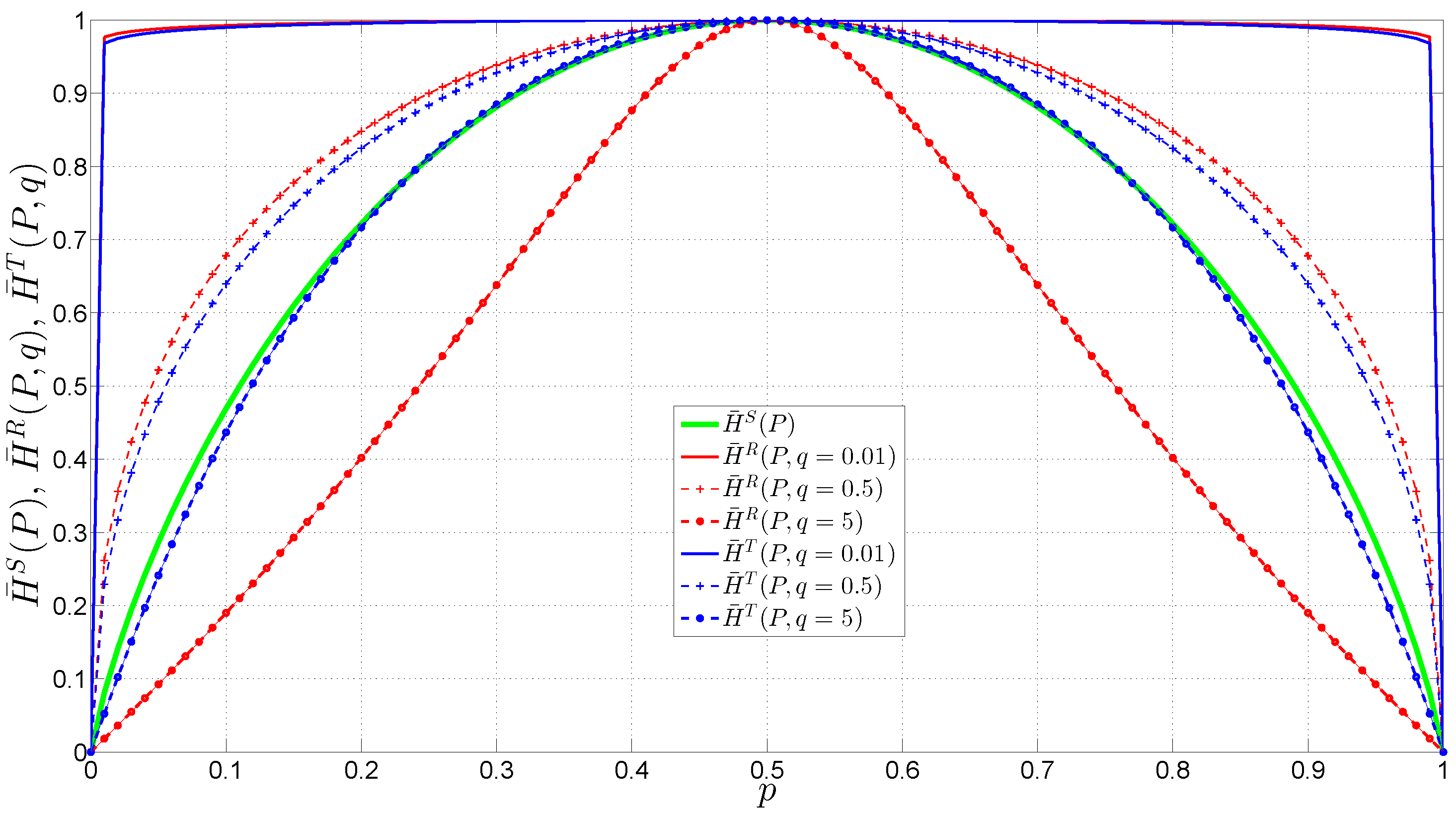
3.1. Entropy Estimators

Let X be a random variable (r.v) which takes values of the set $\{x_1,x_2,...,x_M\},$$p_i:=P(X=x_i)$ the probability of occurrence of $x_i$, and M the cardinality of the finite set; hence, the Shannon entropy is:

$${\widehat{H}}^S\left(P\right)=-\sum _{i=1}^M{p}_{i}log\left(p_i\right).$$

(1)

Based on the Shannon entropy [15], Rényi [16] and Tsallis [17] defined generalized entropies, which are related to the q-deformed algebra

$${\widehat{H}}^R(P,q)=\frac{1}{1-q}log\left(\sum _{i=1}^M{p}_i^q\right)$$

(2)

and

$${\widehat{H}}^T(P,q)=\frac{1}{q-1}\left(1-\sum _{i=1}^M{p}_i^q\right),$$

(3)

where P is a probability distribution. When $q\to 1$ the generalized entropies are reduced to Shannon entropy.

In order to compare the changes of entropy at different times, the entropy is normalized, i.e.,

$$\overline{H}=\frac{\widehat{H}}{{\widehat{H}}_{max}},$$

(4)

where the maximum value of Rényi entropy for the observation vector of size L is given by

$${\widehat{H}}_{max}^R(P,q)=log\left(L\right)$$

(5)

while the maximum of Tsallis entropy is given by

$${\widehat{H}}_{max}^T(P,q)=\frac{1-L^{1-q}}{q-1}.$$

(6)

The parameter q as shown in Equations (2) and (3) is used to make the entropy more or less sensitive to certain events within the distribution, thus modifying the entropy values, and consequently the entropy behavior. In addition, for a specific event with probability p selecting an appropriated value of $q,$ the entropy value with respect to Shannon entropy can be increased (or decreased), see Figure 2.

Figure 2. Entropy estimators (Shannon, Rényi, and Tsallis) for random variable (r.v) X with probabilities $P_x=\{p,(1-p)\}.$

Figure 2. Entropy estimators (Shannon, Rényi, and Tsallis) for random variable (r.v) X with probabilities $P_x=\{p,(1-p)\}.$

3.2. Feature Space

Let $X_t^i,i=1,2,...,p$ be features or random variables of some phenomenon under study and ${\mathbb{R}}^p$ a p-dimensional feature space or space where our variables live. When the phenomenon is observed during a time period T, N observations are collected. These observations can be studied one by one or by group. In our case, the N observations are partitioned into m sequences or windows of length $L.$ For each sequence or time window, a functional $f(•)$ is applied. As our purpose is the study of network traffic and the randomness of the features, we will employ the entropy as $f(•),$ which maps a set of values of a sequence of ${\mathbb{R}}^p$ into a point in ${\mathbb{R}}^p.$

Let $X_j\in {\mathbb{R}}^p,j=1,2,...,N$ be the vectors associated at p features, and $H_i,i=1,..,m,$ the entropies associated at $X^j$ in each sequence. Therefore, we have ${\mathit{X}}_{N\times p}$, a matrix representing the observations, and ${\mathit{H}}_{m\times p}$, the matrix of the entropy of the m sequences.

$${\mathit{X}}_{N\times p}=\left(\begin{array}{cccc}{X}_1^1& X_1^2& \cdots & X_1^p\\ X_2^1& X_2^2& \cdots & X_2^p\\ ⋮& ⋮& ⋮& ⋮\\ X_N^1& X_N^2& \cdots & X_N^p\end{array}\right)\stackrel{f(•)}{\to }{\mathit{H}}_{m\times p}=\left(\begin{array}{cccc}\overline{H}\left(X_1^1\right)& \overline{H}\left(X_1^2\right)& \cdots & \overline{H}\left(X_1^p\right)\\ \overline{H}\left(X_2^1\right)& \overline{H}\left(X_2^2\right)& \cdots & \overline{H}\left(X_2^p\right)\\ ⋮& ⋮& ⋮& ⋮\\ \overline{H}\left(X_m^1\right)& \overline{H}\left(X_m^2\right)& \cdots & \overline{H}\left(X_m^p\right)\end{array}\right)$$

(7)

An ${\mathit{H}}_{m\times p}$ matrix row represents a point in the p-dimensional feature space, and the m points generate a cloud, which characterizes the behavior of p variables of the phenomenon under study. The entropy values will be normalized, $\overline{H}\left(X_i^p\right)\in [0,1],$ in order to perform comparisons between the variables.

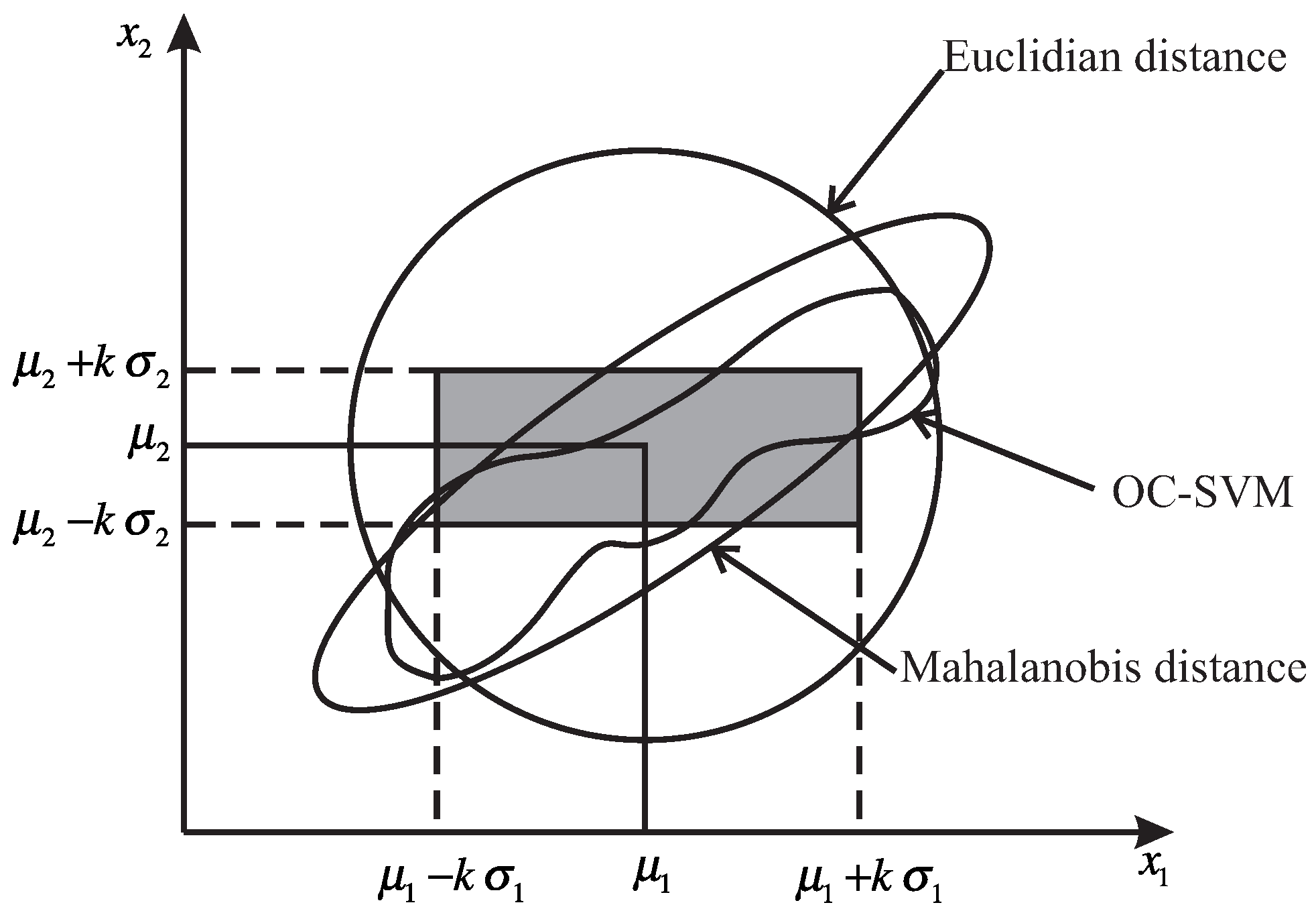
3.3. Mahalanobis Distance

The Mahalanobis distance is defined as [18]: ${\mathbf{d}}^2={(\mathbf{x}-\mathbf{\mu })}^{\prime }{\mathbf{C}}^{-1}(\mathbf{x}-\mathbf{\mu })$ where $\mathbf{x}\in {\mathbb{R}}^p$ is the sample vector, $\mathbf{\mu }\in {\mathbb{R}}^p$ denotes the theoretical mean vector, and $\mathbf{C}\in {\mathbb{R}}^{p\times p}$ denotes the theoretical covariance matrix.

An unbiased sample covariance matrix is

$$\mathbf{S}=\frac{1}{N-1}\sum _{i=1}^N({\mathbf{x}}_i-\overline{\mathbf{x}}){({\mathbf{x}}_i-\overline{\mathbf{x}})}^{\prime },$$

(8)

where the sample mean is

$$\overline{\mathbf{x}}=\frac{1}{N}\sum _{i=1}^N{\mathbf{x}}_i.$$

(9)

Thus, Mahalanobis distance using Equations (8) and (9) is given by:

$${\mathbf{d}}^2={(\mathbf{x}-\overline{\mathbf{x}})}^{\prime }{\mathit{S}}^{-1}(\mathbf{x}-\overline{\mathbf{x}}).$$

(10)

One basic assumption preceding any discussion of the distribution properties of Mahalanobis distance is that the p-multivariate observations involved are the result of a random sampling of a p-variate Gaussian population having a mean vector μ and a covariance matrix C. As μ and C are theoretical values, for a data set containing $x_1,x_2,..,x_N$ samples, $\mathbf{S}$ and $\overline{\mathbf{x}}$ are theirs estimated respectively, and the distribution of ${\mathbf{d}}_i^2({\overline{\mathbf{x}}}_{\mathbf{i}},\mathit{S})$ is given by:

$${\mathbf{d}}_i^2({\overline{\mathbf{x}}}_i,\mathit{S})\sim \left[\frac{{(N-1)}^2}{N}\right]{\beta }_{[\alpha ,p/2,(N-p-1)/2]}$$

(11)

where ${\beta }_{[\alpha ,p/2,(N-p-1)/2]}$ represents a beta distribution with a level of confidence α and parameters $p/2$ and $(N-p-1)/2,$ N is the number of samples and p the number of variables, see [7,19].

If the data sets does not follow a Gaussian distribution, a method to transform non-Gaussian distributed data to a data sets with an approximate Gaussian distribution should be employed. In this paper, the Box-Cox transformation [20] was used. This transformation is a family of power expressions $y^{\left(z\right)}=\frac{x^z-1}{z}$ for $z\ne 0$ and $y^{\left(z\right)}=log\left(x\right)$ for $z=0,$ where z is the transformation parameter that maximizes the Log-likelihood function.

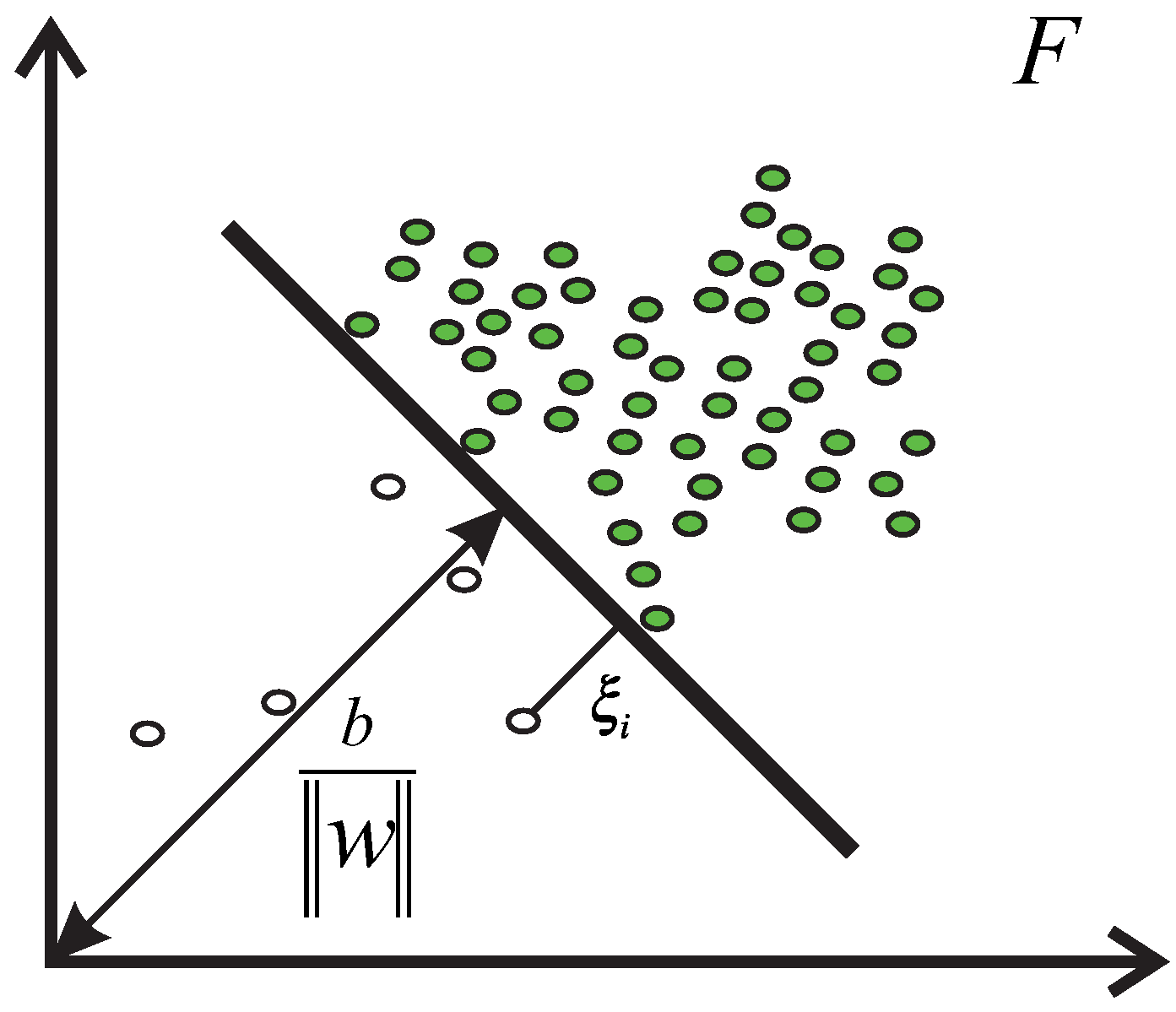
3.4. One Class Support Vector Machine and Mahalanobis Kernel

OC-SVM maps input data ${\mathbf{x}}_1,...,{\mathbf{x}}_N\in A$ (a certain set) into a high dimensional space F (via Kernel $k(\mathbf{x},\mathbf{y})$) and finds the maximal margin hyperplane which best separates the training data from the origin (see Figure 3).

Figure 3. Illustration of One Class Support Vector Machine idea.

Figure 3. Illustration of One Class Support Vector Machine idea.

Theoretical fundamentals of SVM and OC-SVM were established in [21,22,23,24]. In order to separate the data from the origin, the following quadratic program must be solved [21]

$$\underset{w\in F,b\in \mathbb{R},\xi \in {\mathbb{R}}^N}{min}\frac{1}{2}{∥w∥}^2+\frac{1}{\nu N}\sum _i^N{\xi }_i-b$$

(12)

subject to $(w·\phi \left({\mathbf{x}}_i\right))\ge b-{\xi }_i;{\xi }_i\ge 0,\nu \in (0,1],$ where w is the normal vector, φ is a map function $A\to F$, b is the bias, ${\xi }_i$ are nonzero slack variables, ν is the outlier parameter control, and $k(\mathbf{x},\mathbf{y})=(\phi (\mathbf{x}),\phi (\mathbf{y}\left)\right).$ Moreover, the decision function is given by $f\left(\mathbf{x}\right)=sgn\left((w·\phi \left({\mathbf{x}}_i\right))-b\right).$

By applying the kernel function and Lagrangian multiplier (${\alpha }_i$) to the original quadratic program, the solution of Equation (12) creates a decision function:

$$f\left(\mathbf{x}\right)=sgn\left(\sum _i^N{\alpha }_{i}k({\mathbf{x}}_i,\mathbf{x})-b\right),$$

(13)

where $w={\sum }_i{\alpha }_i\phi \left({\mathbf{x}}_i\right)$ and ${\sum }_i{\alpha }_i=1.$

In this work, we used the Mahalanobis kernel (MK), which is defined as: $K(\mathbf{x},\mathbf{y})=exp(-{(\mathbf{x}-\mathbf{y})}^{\prime }C(\mathbf{x}-\mathbf{y}))$, where $\mathbf{C}$ is a positive definite matrix. The Mahalanobis kernel is an extension of the Radial Basis Function kernel (RBF). Namely, by setting $\mathbf{C}=\eta \mathbf{I},$ where $\eta >0$ is a parameter for decision boundary control and $\mathbf{I}$ is the unit matrix, we obtain the RBF kernel:

$$exp(-\eta {∥\mathbf{x}-\mathbf{y}∥}^2).$$

(14)

The Mahalanobis kernel approximation [25] used in this work is:

$$k(\mathbf{x},\mathbf{y})=exp(-\frac{\eta }{p}{(\mathbf{x}-\mathbf{y})}^{\prime }{\mathbf{S}}^{-1}(\mathbf{x}-\mathbf{y})),$$

(15)

where p is the number of variables, and $\mathbf{S}$ is defined by Equation (8).

4. Problem Statement

Let Ω be an Internet traffic data trace, called here Ω-trace, and p the number of random variables $X^i$ representing the traffic features. It is known that the temporal behavior of these variables in the case of “normal” traffic differs from that when there are attacks. On the other hand, in order to characterize these behaviors, entropy can be used, and then instead of studying the traffic features directly, their temporal entropy behaviors $H_i\left(t\right)$ will be studied. We have the following behaviors:

• if Ω-trace was obtained during “normal” network traffic and the outlier exclusion was performed, it will be called β-trace,
• if Ω-trace was obtained during a period containing “normal” traffic plus one or more attacks, it will be called ψ-trace.

The main problem is to find a region, $R_N$ or $R_A$, in the feature space ${\mathbb{R}}^p$ characterizing the temporal behavior of the entropy of the p intrinsic variables associated with a class determined by the traces, i.e.,

• if Ω-trace is β-trace, then a region $R_N$ (“normal” traffic) can be constructed and it will serve to detect the anomalies,
• if Ω-trace is ψ-trace, then a region $R_A$ (abnormal traffic) can be constructed and will serve to classify the anomalies of this class.

Our approach to defining the “normal” $R_N$ or abnormal regions $R_A$ in the feature space uses Mahalanobis distance to construct regular regions (i.e., hyper-ellipsoids) and OC-SVM for non-regular regions.

Figure 4 shows the general architecture of the proposed method, which is composed of three parts: training, detection, and classification. Feature extraction, windowing, entropy calculation, and the Box-Cox transformation (for non-Gaussian data) are performed in the training and detection stages. In the training stage, the different regions in the feature space are defined and the decision functions are obtained. In the detection stage, the “normal” regions $R_N$ and the decision functions are used to detect anomalies in the current traffic. Finally, the anomaly is classified through defined regions $R_A$ of known classes.

Figure 4. General architecture of the proposed method.

Figure 4. General architecture of the proposed method.

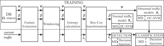
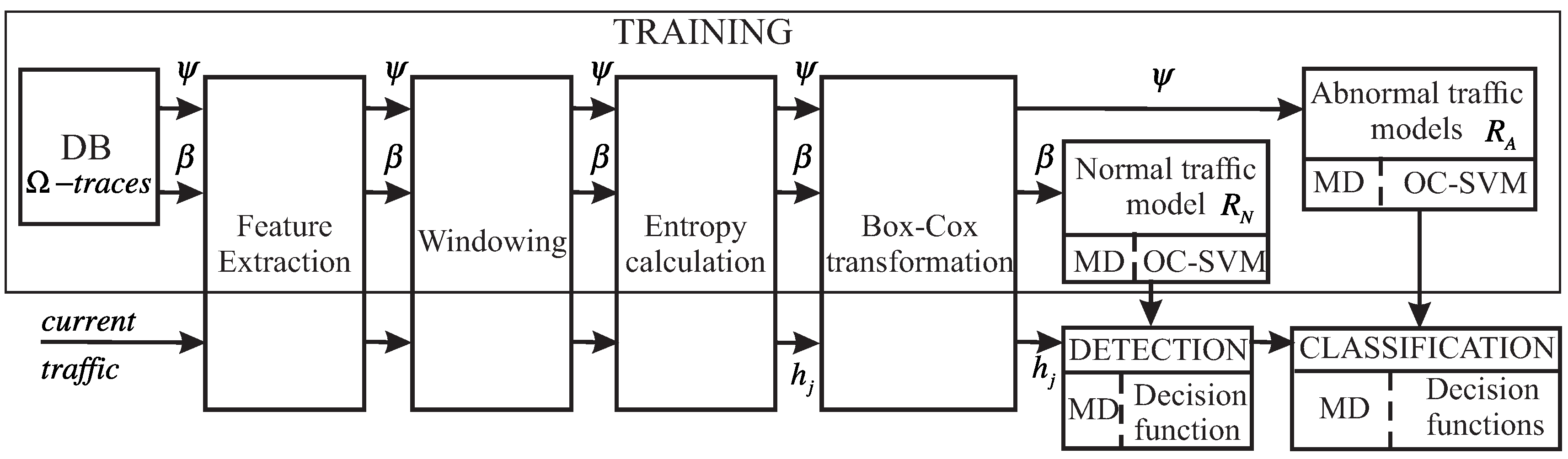
4.1. Algorithm for the Construction of Decision Regions

4.1.1. Training Stage

An Ω-trace is divided into m non-overlapping slots of L packets each. Next, normalized entropy estimates by means of Equations (1)–(3) of each p variable for every j-slot of size L are obtained, using the relative frequencies $\widehat{p_i}=\frac{n_i}{L},$ where $n_i$ is the number of times that the i-element appears in the j-slot. Then, the matrix $\mathit{H}\in {\mathbb{R}}^{m\times p}$ is built as follows:

$${\mathit{H}}_{m\times p}=\left(\begin{array}{cccc}\overline{H}\left(X_1^1\right)& \overline{H}\left(X_1^2\right)& \cdots & \overline{H}\left(X_1^p\right)\\ \overline{H}\left(X_2^1\right)& \overline{H}\left(X_2^2\right)& \cdots & \overline{H}\left(X_2^p\right)\\ ⋮& ⋮& ⋮& ⋮\\ \overline{H}\left(X_m^1\right)& \overline{H}\left(X_m^2\right)& \cdots & \overline{H}\left(X_m^p\right)\end{array}\right)$$

(16)

where $\overline{H}\left(X_j^p\right)$ represents the normalized entropy estimation of the p variable of each j-slot obtained from Ω-trace. The H matrices are inputs of the algorithms for constructing the regions.

Algorithm for constructing regions based on the Mahalanobis distance (MD) method

• Verify that the columns of the H matrix follow a Gaussian distribution. If the data are non-Gaussian, then a transformation is performed so that the new data approximately follow a distribution of this type. In this paper, the Box-Cox transformation was employed.
• Perform the exclusion of outliers of the H matrix. The $LT$ limit for Mahalanobis distance is calculated through Equation (11).
• Calculate the mean vector $\overline{\mathbf{x}}=\{{\overline{x}}_1,{\overline{x}}_2,...,{\overline{x}}_p\},$ where the i-element is the mean of the i-column of the H matrix, see Equation (9).
• Calculate the covariance matrix $\mathbf{S}$ of the H matrix. As the $\mathbf{S}$ matrix is positive definite and Hermitian, all its eigenvalues ${\lambda }_1\ge {\lambda }_2\ge ...\ge {\lambda }_p$ are real and positive, and its eigenvectors ${\gamma }_1,{\gamma }_2,...,{\gamma }_p$ form a set of orthogonal basis vectors that span the p-dimensional vector space.
• Solve the matrix equation $\mathbf{S}\mathbf{\gamma }=\mathbf{\lambda }\mathbf{\gamma }$ according to a specific algorithm in order to obtain the eigenvalues ${\lambda }_i$ and eigenvectors ${\gamma }_i$ of $\mathbf{S}.$
• Finally, define a hyper-ellipsoidal region obtained from the H matrix by means of $\{LT,\overline{\mathbf{x}},\mathbf{\gamma },\mathbf{\lambda }\}.$

Algorithm for constructing regions based on the OC-SVM method

• Verify that the columns of the H matrix follow a Gaussian distribution. If the data are non-Gaussian, then a transformation is performed so that the new data approximately follow a distribution of this type.
• Perform the exclusion of outliers of the H matrix. The $LT$ limit for Mahalanobis distance is calculated through Equation (11).
• Solve Equation (12) via the Sequential Minimal Optimization Algorithm (SMO) [26], using two different kernel functions: RBF and MK. Considering the H matrix as input data, the entropy support vectors $x_i$ and the constants ${\alpha }_i$ and b are obtained.

The algorithm for constructing regions based on the MD or OC-SVM allows regions $R_N$ to be defined if the trace contains “normal” traffic, or regions $R_A$ if the trace contains abnormal traffic.

4.1.2. Detection Stage

• In the current traffic, a j-slot of size L packets is captured, the p features or variables associated to each packet are extracted, and their entropies estimated. With these values, the input vector ${\mathbf{h}}_{\mathbf{j}}$ is built as follows:

  $${\mathbf{h}}_{\mathbf{j}}=\left(\overline{H}\left(X_j^1\right),\overline{H}\left(X_j^2\right),\cdots ,\overline{H}\left(X_j^p\right)\right).$$

  (17)
• The decision function for the MD region is given by Equation (10). If ${\mathbf{d}}_j^2\left({\mathbf{h}}_{\mathbf{j}}\right)\le LT,$ then the j-slot is considered “normal”; otherwise, it is an anomaly.
• The decision function for OC-SVM is expressed by Equation (13). If the decision function maps ${\mathbf{h}}_{\mathbf{j}}$ to $+1,$ then ${\mathbf{h}}_{\mathbf{j}}$ is considered “normal”; otherwise, it is an anomaly.

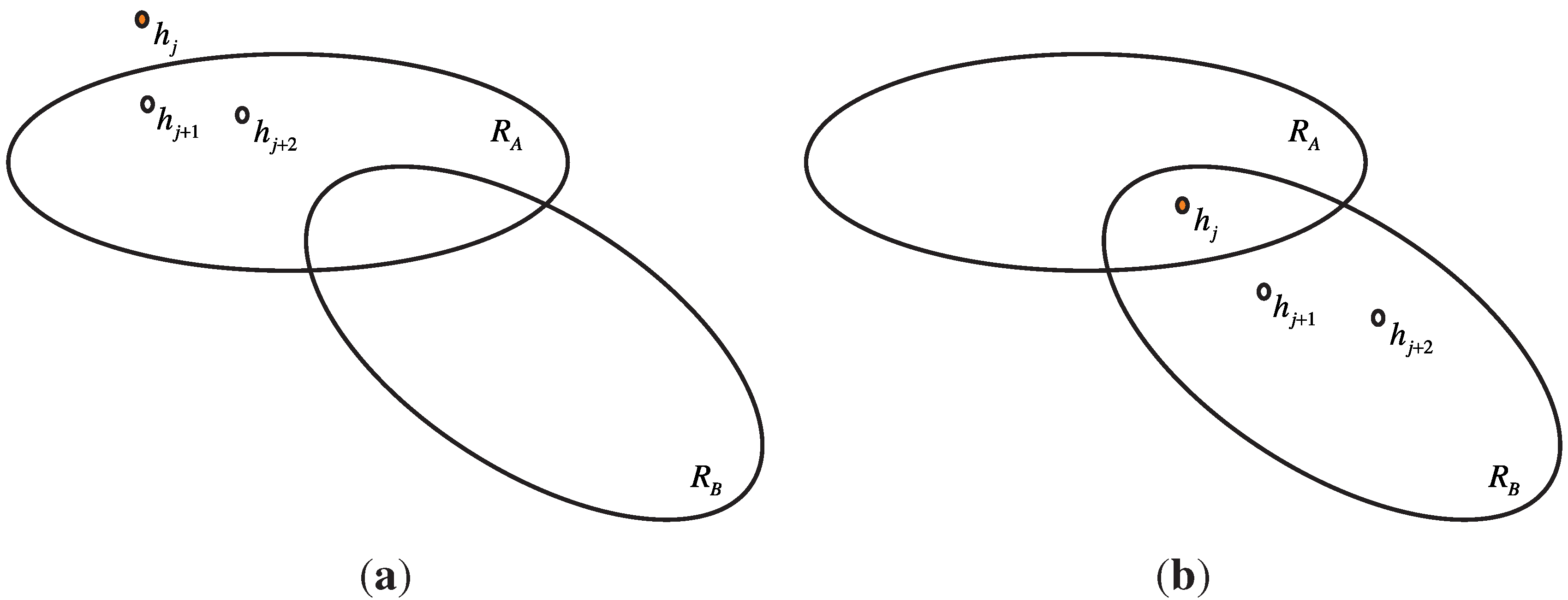
4.1.3. Anomaly Classification Stage

If ${\mathbf{h}}_{\mathbf{j}}$ Equation (17) is outside the “normal” region, i.e., ${\mathbf{h}}_{\mathbf{j}}\notin R_N$, but ${\mathbf{h}}_{\mathbf{j}}\in R_A,$ then the behavior is abnormal and the vector will be classified. Here, ${\mathbf{h}}_{\mathbf{j}}$ is evaluated with all decision functions defined in the training stage.

If ${\mathbf{h}}_{\mathbf{j}}$ is outside all the defined regions or ${\mathbf{h}}_{\mathbf{j}}$ is located in two or more regions, then classification is refined through a criterion based on the k-temporal nearest neighbors algorithm in order to ensure that a point does or does not belong to a specific class.

The principle of the k-temporal nearest neighbors algorithm is that given ${\mathbf{h}}_{\mathbf{j}}$ and its k temporal successors ${\mathbf{h}}_{\mathbf{r}},r=j+1,j+2,..,j+k,$${\mathbf{h}}_{\mathbf{j}}$ using majority vote among these k-temporal nearest neighbors is classified. If ${\mathbf{h}}_{\mathbf{j}}$ is outside all the defined regions and its k temporal successors are as well, then a new attack class will be found or not.

Figure 5 shows an example of the algorithm considering two regions and $k=2$ temporal nearest neighbors. In Figure 5a, point ${\mathbf{h}}_{\mathbf{j}}$ is classified in the $R_A$ region, while in Figure 5b, point ${\mathbf{h}}_{\mathbf{j}}$ is classified in the $R_B$ region.

Figure 5. Use of k-temporal nearest neighbors algorithm in classification stage. (a) ${\mathbf{h}}_{\mathbf{j}}$ is outside all the defined regions; (b) ${\mathbf{h}}_{\mathbf{j}}$ belongs to two or more regions.

Figure 5. Use of k-temporal nearest neighbors algorithm in classification stage. (a) ${\mathbf{h}}_{\mathbf{j}}$ is outside all the defined regions; (b) ${\mathbf{h}}_{\mathbf{j}}$ belongs to two or more regions.

5. Experiments and Results

5.1. Our Data Sets

We evaluated our approach by analyzing its performance over two different experimental databases. The first is from an Academic LAN [27], and is composed of traffic data traces collected over seven days. A trace contains “normal” traffic (${\beta }_1$) and four traces are formed with “normal” traffic plus traffic generated by four real attacks: port scan (${\psi }_1$), and three worms: Blaster (${\psi }_2$), Sasser (${\psi }_3$), and Welchia (${\psi }_4$). The second is a sub-set of the 1998 MIT-DARPA [28] (public set benchmark for testing NIDS), and is composed of one training trace (${\beta }_2$) that was collected over five days of “normal” behavior of the network and four traces containing the traffic generated by Smurf (${\psi }_5$), Neptune (${\psi }_6$), Pod (${\psi }_7$), and portsweep (${\psi }_8$) attacks.

The ${\beta }_1$-trace is composed of “normal” traffic captured over six days. In the training stage, only a day’s traffic is used, and the rest is used for test. A similar procedure is employed for the MIT-DARPA ${\beta }_2$-trace. In the case of anomalous traces, a portion of each ψ-traces were used for training, and the complete traces for the test were employed.

5.2. Traffic Features

According to Section 3.2, the selected features are extracted from the header of each traffic network packet and represented as random variables $X^r;r=1;...;p.$ For our experiments, where attacks generate deviations from the typical behavior of IP and Port addresses, four random variables were selected: $X^1$ source IP addresses, $X^2$ destination IP addresses, $X^3$ source port addresses, and $X^4$ destination port addresses, and the temporal behavior of these features via their entropies ${\mathbf{h}}_{{\mathbf{X}}^{\mathbf{p}}}$ for normal and abnormal traffic were studied.

An Ω-trace is divided into m non-overlapping slots of L packets each. For each i-slot, the normalized entropy for each p variable $\overline{H}\left(X_i^p\right)$ was obtained and the entropy vectors ${\mathbf{h}}_{{\mathbf{X}}^{\mathbf{p}}}=\left(\overline{H}\left(X_1^p\right),\overline{H}\left(X_2^p\right),...,\overline{H}\left(X_m^p\right)\right)$ were constructed. Then, as inputs of the algorithms the following matrices ${\mathit{H}}_{Ip}=\left({{\mathbf{h}}_{{\mathbf{X}}^{\mathbf{1}}}}^{\prime }{{\mathbf{h}}_{{\mathbf{X}}^{\mathbf{2}}}}^{\prime }\right)\in {\mathbb{R}}^{m\times 2},{\mathit{H}}_{Pt}=\left({{\mathbf{h}}_{{\mathbf{X}}^{\mathbf{3}}}}^{\prime }{{\mathbf{h}}_{{\mathbf{X}}^{\mathbf{4}}}}^{\prime }\right),{\mathit{H}}_{IpDPt}=\left({{\mathbf{h}}_{{\mathbf{X}}^{\mathbf{1}}}}^{\prime }{{\mathbf{h}}_{{\mathbf{X}}^{\mathbf{2}}}}^{\prime }{{\mathbf{h}}_{{\mathbf{X}}^{\mathbf{4}}}}^{\prime }\right),{\mathit{H}}_{IpSPt}=\left({{\mathbf{h}}_{{\mathbf{X}}^{\mathbf{1}}}}^{\prime }{{\mathbf{h}}_{{\mathbf{X}}^{\mathbf{2}}}}^{\prime }{{\mathbf{h}}_{{\mathbf{X}}^{\mathbf{3}}}}^{\prime }\right)\in {\mathbb{R}}^{m\times 3},{\mathit{H}}_{IpPt}=\left({{\mathbf{h}}_{{\mathbf{X}}^{\mathbf{1}}}}^{\prime }{{\mathbf{h}}_{{\mathbf{X}}^{\mathbf{2}}}}^{\prime }{{\mathbf{h}}_{{\mathbf{X}}^{\mathbf{3}}}}^{\prime }{{\mathbf{h}}_{{\mathbf{X}}^{\mathbf{4}}}}^{\prime }\right)$ were formed. For estimations of the generalized entropies the selected q-values are $\{0.01,0.5,1.5,2,10\}.$

5.3. The Classifier Metrics

The classifier is a mapping from instances to predicted classes, e.g., in two-class classification problems, each instance (an entropy point in our case) is mapped to one element of the set $\{+1,-1\}$ of positive and negative class labels [29]. Given a classifier and an instance, there are four possible outcomes: $TN$ is the number of correct predictions that an instance is negative, $FP$ is the number of incorrect predictions that an instance is positive, $FN$ is the number of incorrect predictions that an instance is negative, and $TP$ is the number of correct predictions that an instance is positive. With these entries, the following statistics are computed [30]:

• The accuracy (AC) is the proportion of the total number of predictions that were correct: $AC=\frac{TN+TP}{TN+FP+FN+TP}.$
• The sensitivity, detection rate, or true positive rate (TPR) is the proportion of positive cases that were correctly identified: $TPR=\frac{TP}{FN+TP}.$
• The specificity or true negative rate (TNR) is defined as the proportion of negative cases that were classified correctly: $TNR=\frac{TN}{TN+FP}.$
• The false negative rate (FNR) is the proportion of positive cases that were incorrectly classified as negative: $FNR=\frac{FN}{FN+TP}.$

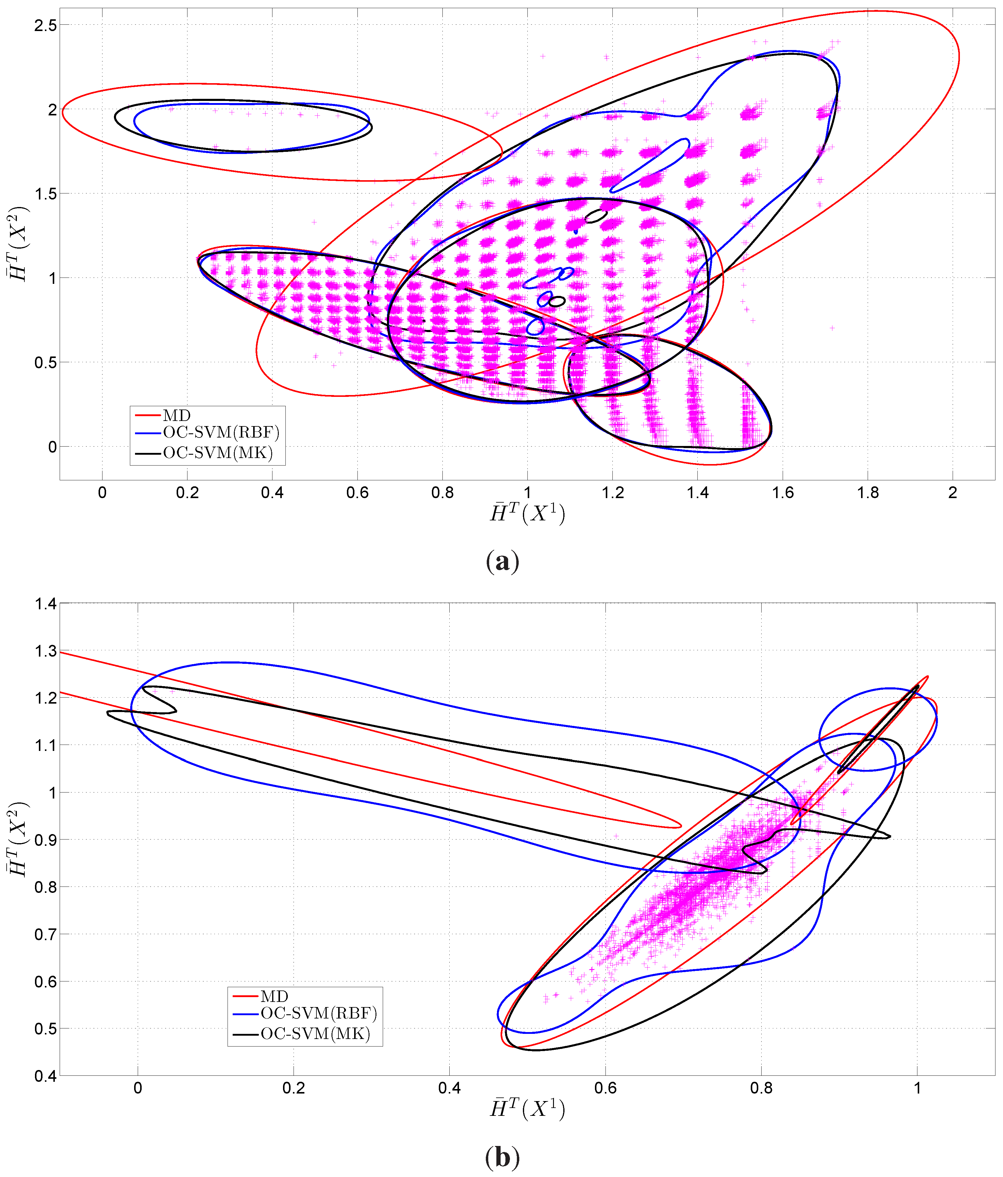
5.4. Detection of Anomalies in Network Traffic

As noted above, anomaly-free traces were divided into m non-overlapping slots of size L (in our case $L=32$) packets. This size was chosen according to the shortest attacks contained in the test traces—around 30 packets—and assuring at least one slot with malicious traffic.

For the input matrices ${\mathit{H}}_{Ip},$ ${\mathit{H}}_{Pt},$ ${\mathit{H}}_{IpSPt},$ ${\mathit{H}}_{IpDPt},$ and ${\mathit{H}}_{IpPt},$ ellipsoids were found through Mahalanobis distance, and non-regular regions were found through OC-SVM Radial Basis Function (RBF) and Mahalanobis kernel (MK). The performance of OC-SVM was evaluated for different combinations of parameters η and ν (see Equations (12), (14), and (15)) in the k-fold cross-validation process with $k=5$. For implementation of OC-SVM, the LIBSVM library [31] was used.

Table 1. True positive and negative rates using Tsallis entropy with $q=0.01$ for different input matrices.

Region	LAN								MIT-DARPA
${\mathit{H}}_{Ip}^T$
	ν	η	# SV	${\beta }_1$	${\psi }_1$	${\psi }_2$	${\psi }_3$	${\psi }_4$	ν	η	# SV	${\beta }_2$	${\psi }_5$	${\psi }_6$	${\psi }_7$	${\psi }_8$
MK	0.1	0.01	167	91.29	100	99.37	81.64	85.97	0.03	0.001	6	99.98	99.91	0.0	92.85	22.22
RBF	9.4	0.01	178	95.78	100	99.24	75.56	85.46	25	0.001	12	99.96	99.91	0.0	92.85	22.22
MD	$\alpha =0.9995$			98.32	100	99.43	66.43	57.58	$\alpha =0.99995$			99.98	99.91	0.0	92.85	22.22
${\mathit{H}}_{Pt}^T$
MK	0.2	0.01	172	92.61	88.88	84.57	61.18	94.09	0.03	0.001	9	99.76	99.39	100	92.85	88.88
RBF	9.4	0.01	194	92.36	88.88	83.34	61.14	91.07	25	0.001	17	99.76	99.82	100	92.85	88.88
MD	$\alpha =0.9995$			98.36	77.77	75.92	60.66	69.02	$\alpha =0.99995$			99.58	99.39	100	92.85	100
${\mathit{H}}_{IpSPt}^T$
MK	0.12	0.01	196	94.96	100	99.59	73.73	98.91	0.05	0.001	10	99.89	99.91	100	92.85	44.44
RBF	9.4	0.01	226	96.77	100	99.73	48.85	99.66	25	0.001	34	99.82	99.91	100	92.85	66.66
MD	$\alpha =0.9995$			98.13	100	99.52	65.89	97.98	$\alpha =0.99995$			99.82	99.91	100	92.85	66.66
${\mathit{H}}_{IpDPt}^T$
MK	0.2	0.01	206	93.62	100	99.47	87.12	99.59	0.05	0.001	12	99.87	99.91	0.0	92.85	88.88
RBF	10.6	0.01	232	96.74	100	99.48	87.93	99.39	25	0.001	30	99.84	99.91	0.0	92.85	100
MD	$\alpha =0.9995$			98.23	100	99.55	69.54	99.25	$\alpha =0.99995$			99.81	99.91	0.0	92.85	100
${\mathit{H}}_{IpPt}^T$
MK	0.12	0.01	206	95.23	100	99.65	79.75	99.59	0.05	0.001	14	99.82	99.91	100	92.85	88.88
RBF	10.4	0.01	291	96.23	100	99.76	86.38	99.75	25	0.001	58	99.56	99.91	100	92.85	100
MD	$\alpha =0.9995$			97.94	100	99.62	69.01	99.23	$\alpha =0.99995$			99.61	99.91	100	92.85	100

Table 1. True positive and negative rates using Tsallis entropy with $q=0.01$ for different input matrices.

Region	LAN								MIT-DARPA
${\mathit{H}}_{Ip}^T$
	ν	η	# SV	${\beta }_1$	${\psi }_1$	${\psi }_2$	${\psi }_3$	${\psi }_4$	ν	η	# SV	${\beta }_2$	${\psi }_5$	${\psi }_6$	${\psi }_7$	${\psi }_8$
MK	0.1	0.01	167	91.29	100	99.37	81.64	85.97	0.03	0.001	6	99.98	99.91	0.0	92.85	22.22
RBF	9.4	0.01	178	95.78	100	99.24	75.56	85.46	25	0.001	12	99.96	99.91	0.0	92.85	22.22
MD	$\alpha =0.9995$			98.32	100	99.43	66.43	57.58	$\alpha =0.99995$			99.98	99.91	0.0	92.85	22.22
${\mathit{H}}_{Pt}^T$
MK	0.2	0.01	172	92.61	88.88	84.57	61.18	94.09	0.03	0.001	9	99.76	99.39	100	92.85	88.88
RBF	9.4	0.01	194	92.36	88.88	83.34	61.14	91.07	25	0.001	17	99.76	99.82	100	92.85	88.88
MD	$\alpha =0.9995$			98.36	77.77	75.92	60.66	69.02	$\alpha =0.99995$			99.58	99.39	100	92.85	100
${\mathit{H}}_{IpSPt}^T$
MK	0.12	0.01	196	94.96	100	99.59	73.73	98.91	0.05	0.001	10	99.89	99.91	100	92.85	44.44
RBF	9.4	0.01	226	96.77	100	99.73	48.85	99.66	25	0.001	34	99.82	99.91	100	92.85	66.66
MD	$\alpha =0.9995$			98.13	100	99.52	65.89	97.98	$\alpha =0.99995$			99.82	99.91	100	92.85	66.66
${\mathit{H}}_{IpDPt}^T$
MK	0.2	0.01	206	93.62	100	99.47	87.12	99.59	0.05	0.001	12	99.87	99.91	0.0	92.85	88.88
RBF	10.6	0.01	232	96.74	100	99.48	87.93	99.39	25	0.001	30	99.84	99.91	0.0	92.85	100
MD	$\alpha =0.9995$			98.23	100	99.55	69.54	99.25	$\alpha =0.99995$			99.81	99.91	0.0	92.85	100
${\mathit{H}}_{IpPt}^T$
MK	0.12	0.01	206	95.23	100	99.65	79.75	99.59	0.05	0.001	14	99.82	99.91	100	92.85	88.88
RBF	10.4	0.01	291	96.23	100	99.76	86.38	99.75	25	0.001	58	99.56	99.91	100	92.85	100
MD	$\alpha =0.9995$			97.94	100	99.62	69.01	99.23	$\alpha =0.99995$			99.61	99.91	100	92.85	100

The regions found are used to detect anomalies in network traffic. Therefore, traces containing traffic generated by different anomalies were used. Each test trace was divided into slots of size L and the estimates of entropy for each selected variable were obtained. For each i-slot the Mahalanobis distance was computed by Equation (10). Likewise, each i-slot was analyzed with OC-SVM decision function Equation (13) and thus it was determined to belong to the non-regular region or not.

Results for anomaly detection of the LAN and MIT-DARPA traces using Tsallis entropy of the features with $q=0.01$ by means of the ellipsoidal (MD) and non-regular (OC-SVM) regions are displayed in Table 1. Additionally, the values of α, η and ν (see Equations (11), (12), (14), and (15)) are shown. The true negative rate for the attack ${\psi }_6$ is 0 or 100, as it is contained in only one slot.

5.5. Classification of Worm Attacks

Each ψ-trace was divided into m non-overlapping slots of size $L.$ For each $i-$slot, $i=1,...,m,$ the estimation of entropy $\overline{H}\left(X_i^r\right)$ of the four selected variables was obtained. Next, ${\mathit{H}}_{Ip},$ ${\mathit{H}}_{Pt},$ ${\mathit{H}}_{IpSPt},$ ${\mathit{H}}_{IpDPt},$ and ${\mathit{H}}_{IpPt}$ matrices were formed. With these matrices, the regions using Mahalanobis distance and OC-SVM with RBF and MK kernel were defined. Figure 6 shows the ellipses and non-regular regions defined in the feature space of IP addresses ${\mathbb{R}}^2$ for each anomalous trace from LAN and MIT-DARPA traces. In Table 2, the selected values of the OC-SVM parameters for the construction of non-regular regions are shown.

We assume that every entropy point outside the normal region is an anomaly; however, not every anomaly belongs to a specific attack class. If a point is an anomaly but the majority of its temporal neighbors are normal, then it is considered normal as well. If a point is an anomaly and the majority of its temporal neighbors belong to a specific anomaly class, then it belongs to this class. Therefore, results were obtained using the k-temporal nearest neighbors algorithm, as in [6].

Table 2. Parameters of OC-SVM for classification of LAN and MIT-DARPA traces with Tsallis entropy, $q=0.01$.

Kernel	LAN												MIT-DARPA
	${\psi }_1$			${\psi }_2$			${\psi }_3$			${\psi }_4$			${\psi }_5$			${\psi }_8$
	ν	η	# SV	ν	η	# SV	ν	η	# SV	ν	η	# SV	ν	η	# SV	ν	η	# SV
${\mathit{H}}_{Ip}^T$
MK	0.01	0.6	3	0.01	0.7	28	0.01	0.9	163	0.01	0.9	115	0.0001	0.1	2	0.01	0.08	2
RBF	0.001	8	3	0.01	13	29	0.01	10	162	0.001	15	33	0.0005	3	2	0.01	25	2
${\mathit{H}}_{Pt}^T$
MK	0.01	0.6	5	0.01	0.7	25	0.01	0.9	35	0.01	0.9	59	0.0001	0.1	3	0.01	0.08	3
RBF	0.001	8	6	0.01	13	48	0.01	10	42	0.001	15	21	0.0005	3	2	0.01	25	3
${\mathit{H}}_{IpSPt}^T$
MK	0.01	0.6	6	0.01	0.7	42	0.01	0.9	189	0.01	0.9	133	0.0001	0.1	2	0.01	0.08	2
RBF	0.001	8	6	0.01	13	66	0.01	10	195	0.001	15	173	0.0005	3	2	0.01	25	3
${\mathit{H}}_{IpDPt}^T$
MK	0.01	0.6	8	0.01	0.7	34	0.01	0.9	173	0.01	0.9	136	0.0001	0.1	2	0.01	0.08	2
RBF	0.001	8	6	0.01	13	49	0.01	10	179	0.001	15	85	0.0005	3	2	0.01	25	5
${\mathit{H}}_{IpPt}^T$
MK	0.01	0.6	8	0.01	0.7	47	0.01	0.9	193	0.01	0.9	148	0.0001	0.1	2	0.01	0.08	4
RBF	0.001	8	5	0.01	13	115	0.01	10	217	0.001	15	283	0.0005	3	2	0.01	25	9

Table 2. Parameters of OC-SVM for classification of LAN and MIT-DARPA traces with Tsallis entropy, $q=0.01$.

Kernel	LAN												MIT-DARPA
	${\psi }_1$			${\psi }_2$			${\psi }_3$			${\psi }_4$			${\psi }_5$			${\psi }_8$
	ν	η	# SV	ν	η	# SV	ν	η	# SV	ν	η	# SV	ν	η	# SV	ν	η	# SV
${\mathit{H}}_{Ip}^T$
MK	0.01	0.6	3	0.01	0.7	28	0.01	0.9	163	0.01	0.9	115	0.0001	0.1	2	0.01	0.08	2
RBF	0.001	8	3	0.01	13	29	0.01	10	162	0.001	15	33	0.0005	3	2	0.01	25	2
${\mathit{H}}_{Pt}^T$
MK	0.01	0.6	5	0.01	0.7	25	0.01	0.9	35	0.01	0.9	59	0.0001	0.1	3	0.01	0.08	3
RBF	0.001	8	6	0.01	13	48	0.01	10	42	0.001	15	21	0.0005	3	2	0.01	25	3
${\mathit{H}}_{IpSPt}^T$
MK	0.01	0.6	6	0.01	0.7	42	0.01	0.9	189	0.01	0.9	133	0.0001	0.1	2	0.01	0.08	2
RBF	0.001	8	6	0.01	13	66	0.01	10	195	0.001	15	173	0.0005	3	2	0.01	25	3
${\mathit{H}}_{IpDPt}^T$
MK	0.01	0.6	8	0.01	0.7	34	0.01	0.9	173	0.01	0.9	136	0.0001	0.1	2	0.01	0.08	2
RBF	0.001	8	6	0.01	13	49	0.01	10	179	0.001	15	85	0.0005	3	2	0.01	25	5
${\mathit{H}}_{IpPt}^T$
MK	0.01	0.6	8	0.01	0.7	47	0.01	0.9	193	0.01	0.9	148	0.0001	0.1	2	0.01	0.08	4
RBF	0.001	8	5	0.01	13	115	0.01	10	217	0.001	15	283	0.0005	3	2	0.01	25	9

Figure 6. Worm attack regions in 2D space. (a) Worm attack regions from LAN traces in 2D space ($L=32$); (b) Worm attack regions from MIT-DARPA traces in 2D space ($L=32$).

Figure 6. Worm attack regions in 2D space. (a) Worm attack regions from LAN traces in 2D space ($L=32$); (b) Worm attack regions from MIT-DARPA traces in 2D space ($L=32$).

In Figure 7, the impact of the k-value of k-temporal nearest neighbors algorithm on the classification for LAN traces using Tsallis entropy of Ips and ports variables with $q=0.01$ is shown. TPR values are results of the classifiers trained with β-traces and TNR values are results of the classifiers trained with ψ-traces.

Figure 7. Impact of the k-value of k-temporal nearest neighbors algorithm on the classification.

Figure 7. Impact of the k-value of k-temporal nearest neighbors algorithm on the classification.

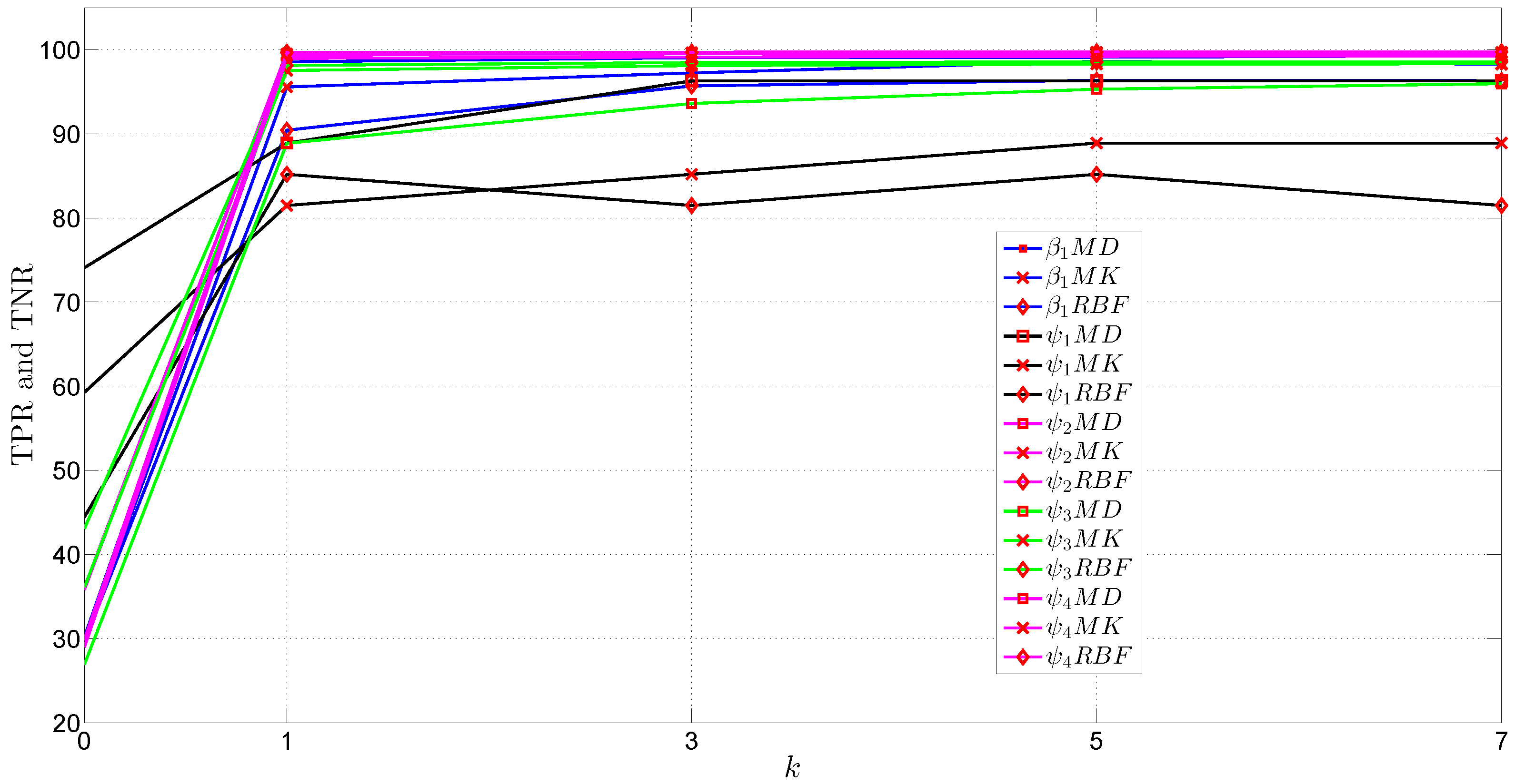
6. Discussion of the Experimental Results

Our approach, see Figure 4, based on mathematical tools such as Mahalanobis distance, covariance matrix, OC-SVM, and the k-temporal nearest neighbors algorithm allows the construction of different regions (regular and non-regular), which encompass the behaviors of the four selected features. These regions allow:

• the classification of an entropy vector as normal or abnormal, and
• the classification of an abnormal entropy vector based on known attacks.

The effects of the number of features—input matrices—on the true positive and negative rate is shown in Table 1. Although in general more variables mean better results, a particular case occurred in trace ${\psi }_3,$ where the use of three variables was better than four.

For anomalous ψ-traces, experimental results show that the true negative rate for $q<1$ is higher than the results for $q>1.$ Figure 8 shows the behavior of the true negative rate using four variables for different q values of Tsallis entropy using OC-SVM with RBF kernel.

The runtime of the decision function of OC-SVM, see Equation (13), is determined by the number of support vectors ($x_i$). In this regard, the Mahalanobis kernel has a smaller number of support vectors than RBF kernel in the MIT-DARPA traces. For LAN traces, the kernel that uses fewer support vectors is RBF.

When a sequence of anomalies occur in network traffic, the entropy values begin to move away from the “normal” region to a new region. This transient state affects classification when few neighbors $(k\le 2)$ of the k-temporal nearest neighbors algorithm are selected. Choosing a larger k-value mitigates the effect of this transient, and therefore, the classification rate will stabilize. Table 3 shows that when the number of neighbors is increased, the classification accuracy in the network LAN is increased as well. Using the k-temporal nearest neighbors method, classification is improved; however, classification is performed $k-$slots later. Experimental results showed that for values of k between 3 and 5, the accuracy classification reaches a steady state, and the delay time is not significant.

Figure 8. True negative rate for different values of q parameter of Tsallis entropy using OC-SVM with RBF kernel.

Figure 8. True negative rate for different values of q parameter of Tsallis entropy using OC-SVM with RBF kernel.

Table 3. Accuracy of the classification of LAN and MIT-DARPA traces vs. different k-values of k-temporal nearest neighbors, using $q=0.01$ in LAN traces, and $q=0.5$ in MIT-DARPA traces for generalized entropies.

k	OC-SVM MK			OC-SVM RBF			MD
	${\mathit{H}}_{IpPt}^T$	${\mathit{H}}_{IpPt}^R$	${\mathit{H}}_{IpPt}^S$	${\mathit{H}}_{IpPt}^T$	${\mathit{H}}_{IpPt}^R$	${\mathit{H}}_{IpPt}^S$	${\mathit{H}}_{IpPt}^T$	${\mathit{H}}_{IpPt}^R$	${\mathit{H}}_{IpPt}^S$
	LAN
0	32.4027	61.3592	38.9434	33.8506	66.0973	40.3794	30.1646	55.5757	33.7279
1	98.7503	98.8099	97.9229	98.7698	98.6869	98.9292	96.9534	96.1043	95.4036
3	99.1611	99.1210	98.2794	99.1871	99.0668	99.0142	98.0583	97.3197	96.3232
5	99.3079	99.2017	98.3141	99.2695	99.1844	99.0906	98.4566	97.7738	96.6380
7	99.2917	99.2695	98.3856	99.2716	99.2066	99.0771	98.6311	98.1488	96.8542
	MIT-DARPA
0	24.2665	25.6156	23.8716	14.1701	8.7415	9.9645	86.7067	92.3433	93.2046
1	99.9595	98.6699	99.9167	99.2338	99.9690	99.7382	99.9952	99.9976	99.9976
3	99.7430	99.6359	99.9357	99.8025	99.7596	99.7644	99.9952	99.9976	99.9976
5	99.6573	99.6097	99.9310	99.8524	99.6264	99.6811	99.9928	99.9952	99.9952
7	99.4670	99.6407	99.9286	99.8477	99.3908	99.4694	99.9904	99.9928	99.9928

Table 3. Accuracy of the classification of LAN and MIT-DARPA traces vs. different k-values of k-temporal nearest neighbors, using $q=0.01$ in LAN traces, and $q=0.5$ in MIT-DARPA traces for generalized entropies.

k	OC-SVM MK			OC-SVM RBF			MD
	${\mathit{H}}_{IpPt}^T$	${\mathit{H}}_{IpPt}^R$	${\mathit{H}}_{IpPt}^S$	${\mathit{H}}_{IpPt}^T$	${\mathit{H}}_{IpPt}^R$	${\mathit{H}}_{IpPt}^S$	${\mathit{H}}_{IpPt}^T$	${\mathit{H}}_{IpPt}^R$	${\mathit{H}}_{IpPt}^S$
	LAN
0	32.4027	61.3592	38.9434	33.8506	66.0973	40.3794	30.1646	55.5757	33.7279
1	98.7503	98.8099	97.9229	98.7698	98.6869	98.9292	96.9534	96.1043	95.4036
3	99.1611	99.1210	98.2794	99.1871	99.0668	99.0142	98.0583	97.3197	96.3232
5	99.3079	99.2017	98.3141	99.2695	99.1844	99.0906	98.4566	97.7738	96.6380
7	99.2917	99.2695	98.3856	99.2716	99.2066	99.0771	98.6311	98.1488	96.8542
	MIT-DARPA
0	24.2665	25.6156	23.8716	14.1701	8.7415	9.9645	86.7067	92.3433	93.2046
1	99.9595	98.6699	99.9167	99.2338	99.9690	99.7382	99.9952	99.9976	99.9976
3	99.7430	99.6359	99.9357	99.8025	99.7596	99.7644	99.9952	99.9976	99.9976
5	99.6573	99.6097	99.9310	99.8524	99.6264	99.6811	99.9928	99.9952	99.9952
7	99.4670	99.6407	99.9286	99.8477	99.3908	99.4694	99.9904	99.9928	99.9928

Considering packet sizes of 60 bytes in a 100Mbs network to capture a slot of 32 packets, the time required is $\frac{32\times 60\times 8}{100Mbs}=153.6\mu S.$ Using a PC with Intel Core i7 3.4 Ghz and 16 G of RAM, a C-implementation of the proposed method using MD and including the decision function required computation times of no more than $5\mu s.$ Therefore, the proposed method can be implemented in real time.

7. Conclusions

In this paper, an approach was proposed for detecting and classifying Internet traffic anomalies using the entropy of selected features, Mahalanobis distance, and OC-SVM with two kernels: RBF and Mahalanobis kernel. Regular and non-regular regions were built with “normal” traffic from training data. For detection of an anomaly, computation times in order of few $\mu s$ were obtained; consequently, these results are very significant for real time implementations.

In the detection stage, for all traces the highest true positive and negative rates (99.35% for “normal” traffic and up to 99.83% for anomalous traffic) were obtained, using the generalized entropies (particularly Tsallis entropy) with $q=0.01,$ and OC-SVM with RBF kernel. However, the optimal q is not addressed in this work.

In the classification stage:

• For Academic LAN traces, using Tsallis entropy with $q=0.01$, OC-SVM with Mahalanobis kernel, and considering $k=5$ for the k-temporal nearest neighbor algorithm the highest results of accuracy (99.30%) were obtained.
• For MIT-DARPA traces, using the MD method, Rényi entropy with $q=0.5,$ and $k\ge 1$ for the k-temporal nearest neighbor algorithm the highest results of accuracy (99.99%) were obtained.

References

1. Chandola, V.; Banerjee, A.; Kumar, V. Anomaly Detection: A Survey. ACM Comput. Surv. 2009, 41. [Google Scholar] [CrossRef]
2. Lakhina, A.; Crovella, M.; Diot, C. Mining Anomalies Using Traffic Feature Distributions. In Proceedings of the 2005 Conference on Applications, Technologies, Architectures, and Protocols for Computer Communications, Philadelphia, PA, USA, 22–26 August 2005; Volume 35, pp. 217–228.
3. Wagner, A.; Plattner, B. Entropy Based Worm and Anomaly Detection in Fast IP Networks. In Proceedings of the 14th IEEE International Workshops on Enabling Technologies: Infrastructure for Collaborative Enterprise, Linköping, Sweden, 13–15 June 2005; pp. 172–177.
4. Xu, K.; Zhang, Z.L.; Bhattacharyya, S. Profiling Internet Backbone Traffic: Behavior Models and Applications. In Proceedings of the 2005 conference on Applications, Technologies, Architectures, and Protocols for Computer Communications, Philadelphia, PA, USA, 22–26 August 2005; Volume 35, pp. 169–180.
5. Santiago-Paz, J.; Torres-Roman, D.; Velarde-Alvarado, P. Detecting anomalies in network traffic using Entropy and Mahalanobis distance. In Proceedings of the 2012 22nd International Conference on Electrical Communications and Computers (CONIELECOMP), Cholula, Mexico, 27–29 February 2012; pp. 86–91.
6. Santiago-Paz, J.; Torres-Roman, D. Characterization of worm attacks using entropy, Mahalanobis distance and K-nearest neighbors. In Proceedings of the 2014 International Conference on Electronics, Communications and Computers (CONIELECOMP), Cholula, Mexico, 26–28 February 2014; pp. 200–205.
7. Mason, R.L.; Young, J.C. Multivariate Statistical Process Control with Industrial Applications; Siam: Philadelphia, PA, USA, 2002; Volume 9. [Google Scholar]
8. Li, K.L.; Huang, H.K.; Tian, S.F.; Xu, W. Improving one-class SVM for anomaly detection. In Proceedings of the 2003 International Conference on Machine Learning and Cybernetics, Xi’an, China, 2–5 November 2003; Volume 5, pp. 3077–3081.
9. Zhang, R.; Zhang, S.; Lan, Y.; Jiang, J. Network anomaly detection using one class support vector machine. In Proceedings of the International MultiConference of Engineers and Computer Scientists (IMECS), Hong Kong, China, 19–21 March 2008.
10. Nychis, G.; Sekar, V.; Andersen, D.G.; Kim, H.; Zhang, H. An Empirical Evaluation of Entropy-based Traffic Anomaly Detection. In Proceedings of the 8th ACM SIGCOMM Conference on Internet Measurement, Vouliagmeni, Greece, 20–22 October 2008; ACM: New York, NY, USA, 2008; pp. 151–156. [Google Scholar]
11. Ziviani, A.; Gomes, A.T.A.; Monsores, M.L.; Rodrigues, P.S. Network anomaly detection using nonextensive entropy. IEEE Commun. Lett. 2007, 11, 1034–1036. [Google Scholar] [CrossRef]
12. Tellenbach, B.; Burkhart, M.; Schatzmann, D.; Gugelmann, D.; Sornette, D. Accurate Network Anomaly Classification with Generalized Entropy Metrics. Comput. Netw. 2011, 55, 3485–3502. [Google Scholar] [CrossRef]
13. Ma, X.; Chen, Y. DDoS Detection method based on chaos analysis of network traffic entropy. Commun. Lett. IEEE 2014, 18, 114–117. [Google Scholar] [CrossRef]
14. Bhuyan, M.H.; Bhattacharyya, D.; Kalita, J. An empirical evaluation of information metrics for low-rate and high-rate DDoS attack detection. Pattern Recognit. Lett. 2015, 51, 1–7. [Google Scholar] [CrossRef]
15. Shannon, C.E. A Mathematical Theory of Communication. Bell Syst. Tech. J. 1948, 27, 379–423. [Google Scholar] [CrossRef]
16. Rényi, A. Probability Theory; North-Holland Series in Applied Mathematics and Mechanics; Elsevier: Amsterdam, The Netherlands, 1970. [Google Scholar]
17. Tsallis, C. Possible generalization of Boltzmann-Gibbs statistics. J. Stat. Phys. 1988, 52, 479–487. [Google Scholar] [CrossRef]
18. Mahalanobis, P.C. On the Generalised Distance in Statistics; Proceedings of the National Institute of Science: Calcutta, India, 1936; Volume 2, pp. 49–55. [Google Scholar]
19. Tracy, N.D. Multivariate control charts for individual observations. J. Qual. Technol. 1992, 24, 88–95. [Google Scholar]
20. Box, G.E.P.; Cox, D.R. An Analysis of Transformations. J. R. Stat. Soc. B Stat. Methodol. 1964, 26, 211–252. [Google Scholar]
21. Schölkopf, B.; Platt, J.C.; Shawe-Taylor, J.C.; Smola, A.J.; Williamson, R.C. Estimating the Support of a High-Dimensional Distribution. Neural Comput. 2001, 13, 1443–1471. [Google Scholar] [CrossRef] [PubMed]
22. Boser, B.E.; Guyon, I.M.; Vapnik, V.N. A Training Algorithm for Optimal Margin Classifiers. In Proceedings of the Fifth Annual Workshop on Computational Learning Theory, Pittsburgh, PA, USA, 27–29 July 1992; ACM: New York, NY, USA, 1992; pp. 144–152. [Google Scholar]
23. Vapnik, V.N. The Nature of Statistical Learning Theory; Springer: New York, NY, USA, 1995. [Google Scholar]
24. Schölkopf, B.; Burges, C.J.C.; Smola, A.J. Advances in Kernel Methods: Support Vector Learning; MIT Press: Cambridge, MA, USA, 1999. [Google Scholar]
25. Abe, S. Training of Support Vector Machines with Mahalanobis Kernels. In Artificial Neural Networks: Formal Models and Their Applications—ICANN 2005; Lecture Notes in Computer Science; Duch, W., Kacprzyk, J., Oja, E., Zadrożny, S., Eds.; Springer: Berlin, Germany, 2005; Volume 3697, pp. 571–576. [Google Scholar]
26. Platt, J. Sequential Minimal Optimization: A Fast Algorithm for Training Support Vector Machines; Technical Report MSR-TR-98-14; Microsoft Research: Redmond, WA, USA, 1998. [Google Scholar]
27. Velarde-Alvarado, P.; Vargas-Rosales, C.; Torres-Román, D.; Martinez-Herrera, A. Entropy-based profiles for intrusion detection in LAN traffic. Adv. Artif. Intell. 2008, 40, 119–130. [Google Scholar]
28. Kendall, K. A Database of Computer Attacks for the Evaluation of Intrusion Detection Systems; Technical Report, DTIC Document; Massachusetts Institute of Technology: Cambridge, MA, USA, 1999. [Google Scholar]
29. Fawcett, T. An Introduction to ROC Analysis. Pattern Recognit. Lett. 2006, 27, 861–874. [Google Scholar] [CrossRef]
30. Kohavi, R.; Provost, F. Glossary of Terms. J. Mach. Learn. 1998, 30, 271–274. [Google Scholar]
31. Chang, C.C.; Lin, C.J. LIBSVM: A Library for Support Vector Machines. ACM Trans. Intell. Syst. Technol. 2011, 2. [Google Scholar] [CrossRef]