Contribution to Transfer Entropy Estimation via the k-Nearest-Neighbors Approach

Abstract

This paper deals with the estimation of transfer entropy based on the k-nearest neighbors (k-NN) method. To this end, we first investigate the estimation of Shannon entropy involving a rectangular neighboring region, as suggested in already existing literature, and develop two kinds of entropy estimators. Then, applying the widely-used error cancellation approach to these entropy estimators, we propose two novel transfer entropy estimators, implying no extra computational cost compared to existing similar k-NN algorithms. Experimental simulations allow the comparison of the new estimators with the transfer entropy estimator available in free toolboxes, corresponding to two different extensions to the transfer entropy estimation of the Kraskov–Stögbauer–Grassberger (KSG) mutual information estimator and prove the effectiveness of these new estimators.

1. Introduction

Transfer entropy (TE) is an information-theoretic statistic measurement, which aims to measure an amount of time-directed information between two dynamical systems. Given the past time evolution of a dynamical system $\mathcal{A}$, TE from another dynamical system $\mathcal{B}$ to the first system $\mathcal{A}$ is the amount of Shannon uncertainty reduction in the future time evolution of $\mathcal{A}$ when including the knowledge of the past evolution of $\mathcal{B}$. After its introduction by Schreiber [1], TE obtained special attention in various fields, such as neuroscience [2–8], physiology [9–11], climatology [12] and others, such as physical systems [13–17].

More precisely, let us suppose that we observe the output X_i ∈ ℝ, i ∈ ℤ, of some sensor connected to $\mathcal{A}$. If the sequence X is supposed to be an m-th order Markov process, i.e., if considering subsequences $X_i^{(k)}=(X_{i-k+1},X_{i-k+2},\cdots X_i),k>0$, the probability measure ${\mathcal{P}}_X$ (defined on measurable subsets of real sequences) attached to X fulfills the m-th order Markov hypothesis:

$$\forall i:\forall m^{\prime }>m:{\mathrm{d}\mathcal{P}}_{X_{i+1}|X_i^{(m)}}\left(x_{i+1}|x_i^{(m)}\right)={\mathrm{d}\mathcal{P}}_{X_{i+1}|X_i^{(m^{\prime })}}\left(x_{i+1}|x_i^{(m^{\prime })}\right),x_{i+1}\in ℝ,x_i^{(k)}\in {ℝ}^k,$$

(1)

then the past information $X_i^{(m)}$ (before time instant i + 1) is sufficient for a prediction of X_i+k, k ≥ 1, and can be considered as an m-dimensional state vector at time i (note that, to know from X the hidden dynamical evolution of $\mathcal{A}$, we need a one-to-one relation between $X_i^{(m)}$ and the physical state of $\mathcal{A}$ at time i). For the sake of clarity, we introduce the following notation: $\left(X_i^p,X_i^{-},Y_i^{-}\right)$, i = 1, 2, …, N, is an independent and identically distributed (IID) random sequence, each term following the same distribution as a random vector (X^p, X⁻, Y⁻) ∈ ℝ^1+m+n whatever i (in X^p, X⁻, Y⁻, the upper indices “p” and “-” correspond to “predicted” and “past”, respectively). This notation will substitute for the notation $\left(X_{i+1},X_i^{(m)},Y_i^{(n)}\right)$, i = 1, 2, …, N, and we will denote by ${\mathcal{S}}_{X^p,X^{-},Y^{-}}$, ${\mathcal{S}}_{X^p,X^{-}}$, ${\mathcal{S}}_{X^{-},Y^{-}}$ and ${\mathcal{S}}_{X^{-}}$ the spaces in which (X^p, X⁻, Y⁻), (X^p, X⁻), (X⁻, Y⁻) and X⁻ are respectively observed.

Now, let us suppose that a causal influence exists from $\mathcal{B}$ on $\mathcal{A}$ and that an auxiliary random process Y_i ∈ ℝ, i ∈ ℤ, recorded from a sensor connected to $\mathcal{B}$, is such that, at each time i and for some n > 0, $Y_i^{-}\triangleq Y_i^{(n)}$ is an image (not necessarily one-to-one) of the physical state of $\mathcal{B}$. The negation of this causal influence implies:

$$\forall (m>0,n>0:\forall i:{\mathrm{d}\mathcal{P}}_{X_i^p|X_i^{(m)}}\left(x_i^p|x_i^{(m)}\right)={\mathrm{d}\mathcal{P}}_{X_i^p|X_i^{(m)},Y_i^{(n)}}\left(x_i^p|x_i^{(m)},y_i^{(n)}\right).$$

(2)

If Equation (2) holds, it is said that there is an absence of information transfer from $\mathcal{B}$ to $\mathcal{A}$. Otherwise, the process X can be no longer considered strictly a Markov process. Let us suppose the joint process (X, Y) is Markovian, i.e., there exist a given pair (m′, n′), a transition function f and an independent random sequence ei, i ∈ ℤ, such that ${[X_{i+1},Y_{i+1}]}^T=f\left(X_i^{(m^{\prime })},Y_i^{(m^{\prime })},e_{i+1}\right)$, where the random variable e_i+1 is independent of the past random sequence (X_j, Y_j, e_j), j ≤ i, whatever i. As $X_i=g\left(X_i^{(m)},Y_i^{(m)}\right)$ where g is clearly a non-injective function, the pair $\left\{\left(X_i^{(m)},Y_i^{(n)}\right),X_i\right\}$, i ∈ ℤ, corresponds to a hidden Markov process, and it is well known that this observation process is not generally Markovian.

The deviation from this assumption can be quantified using the Kullback pseudo-metric, leading to the general definition of TE at time i:

$${\mathrm{TE}}_{Y\to X,i}={\displaystyle {\int }_{{ℝ}^{m+n+1}}\log \left[\frac{d{\mathcal{P}}_{X_i^p|X_i^{-},Y_i^{-}}\left(x_i^p|x_i^{-},y_i^{-}\right)}{d{\mathcal{P}}_{X_i^p|X_i^{-}}\left(x_i^p|x_i^{-}\right)}\right]d{\mathcal{P}}_{X_i^p,X_i^{-},Y_i^{-}}\left(x_i^p,x_i^{-},y_i^{-}\right)},$$

(3)

where the ratio in Equation (3) corresponds to the Radon–Nikodym derivative [18,19] (i.e., the density) of the conditional measure $d{\mathcal{P}}_{X_i^p|X_i^{-},Y_i^{-}}\left(\cdot |x_i^{-},y_i^{-}\right)$ with respect to the conditional measure $d{\mathcal{P}}_{X_i^p|X_i^{-}}\left(\cdot |x_i^{-}\right)$ Considering “log” as the natural ogarithm, information is measured in natural (nats). Now, given two observable scalar random time series X and Y with no a priori given model (as is generally the case), if we are interested in defining some causal influence from Y to X through TE analysis, we must specify the dimensions of the past information vectors X⁻ and Y⁻, i.e., m and n. Additionally, even if we impose them, it is not evident that all of the coordinates in $X_i^{(m)}$ and $Y_i^{(n)}$ will be useful. To deal with this issue, variable selection procedures have been proposed in the literature, such as uniform and non-uniform embedding algorithms [20,21].

If the joint probability measure ${\mathcal{P}}_{X_i^p,X_i^{-},Y_i^{-}}\left(x_i^p,x_i^{-},y_i^{-}\right)$ is derivable with respect to the Lebesgue measure µ^n+m+1 in ℝ^1+m+n (i.e., if ${\mathcal{P}}_{X_i^p,X_i^{-},Y_i^{-}}$ is absolutely continuous with respect to µ^n++m+1), then the pdf (joint probability density function) $p_{X_i^p,X_i^{-},Y_i^{-}}\left(x_i^p,x_i^{-},y_i^{-}\right)$ and also the pdf for each subset of $\left\{X_i^p,X_i^{-},Y_i^{-}\right\}$ exist, and TE_Y→X,i can then be written (see Appendix A):

$$\begin{array}{c}{\mathrm{TE}}_{Y\to X,i}=-E\left[\log \left(p_{X_i^{-},Y_i^{-}}(X_i^{-},Y_i^{-})\right)\right]-E\left[\log \left(p_{X_i^p,X_i^{-}}(X_i^p,Y_i^{-})\right)\right]\\ +E\left[\log \left(p_{X_i^p,X_i^{-},Y_i^{-}}(X_i^p,X_i^{-},Y_i^{-})\right)\right]+E\left[\log \left(p_{X_i^{-}}(X_i^{-})\right)\right]\end{array}$$

(4)

or:

$${\mathrm{TE}}_{Y\to X,i}=\mathcal{H}(X_i^{-},Y_i^{-})+\mathcal{H}(X_i^p,X_i^{-})-\mathcal{H}(X_i^p,X_i^{-},Y_i^{-})-\mathcal{H}(X_i^{-}),$$

(5)

where $\mathscr{H}$(U) denotes the Shannon differential entropy of a random vector U. Note that, if the processes Y and X are assumed to be jointly stationary, for any real function g : ℝ^m+n+1 → ℝ, the expectation $E\left[g\left(X_{i+1},X_i^{(m)},Y_i^{(m)}\right)\right]$ does not depend on i. Consequently, TE_Y→X,i does not depend on i (and so can be simply denoted by TE_Y→X), nor all of the quantities defined in Equations (3) to (5). In theory, TE is never negative and is equal to zero if and only if Equation (2) holds.

According to Definition (3), TE is not symmetric, and it can be regarded as a conditional mutual information (CMI) [3,22] (sometimes also named partial mutual information (PMI) in the literature [23]). Recall that mutual information between two random vectors X and Y is defined by:

$$\mathcal{I}(X;Y)=\mathcal{H}(X)+\mathcal{H}(Y)-\mathcal{H}(X,Y),$$

(6)

and TE can be also written as:

$${\mathrm{TE}}_{Y\to X}=\mathcal{I}(X^p,Y^{-}|X^{-}).$$

(7)

Considering the estimation $\widehat{{\mathrm{TE}}_{Y\to X}}$ of TE, TE_Y→X, as a function defined on the set of observable occurrences (x_i, y_i), i = 1, …, N, of a stationary sequence (X_i, Y_i), i = 1, …, N, and Equation (5), a standard structure for the estimator is given by (see Appendix B):

$$\begin{array}{l}\widehat{{\mathrm{TE}}_{Y\to X}}=\mathcal{H}\widehat{(X^{-},Y^{-})}+\mathcal{H}\widehat{(X^p,X^{-})}-\mathcal{H}\widehat{(X^p,X^{-},Y^{-})}-\mathcal{H}\widehat{(X^{-})}\\ =-\frac{1}{N}{\displaystyle \sum _{n=1}^N\log \widehat{(p_{U_1}(u_{1n}))}}-\frac{1}{N}{\displaystyle \sum _{n=1}^N\log \widehat{(p_{U_2}(u_{2n}))}}+\frac{1}{N}{\displaystyle \sum _{n=1}^N\log \widehat{(p_{U_3}(u_{3n}))}}\\ +\frac{1}{N}{\displaystyle \sum _{n=1}^N\log \widehat{(p_{U_4}(u_{4n}))}},\end{array}$$

(8)

where U₁, U₂, U₃ and U₄ stand respectively for (X⁻, Y⁻), (X^p, X⁻), (X^p, X⁻, Y⁻) and X⁻. Here, for each n, $\log \widehat{(p_U(u_n))}$ is an estimated value of log (p_U (u_n)) computed as a function f_n (u₁, …, u_N) of the observed sequence u_n, n = 1, …, N. With the k-NN approach addressed in this study, f_n (u₁, …, u_N) depends explicitly only on u_n and on its k nearest neighbors. Therefore, the calculation of $\widehat{\mathcal{H}(U)}$ definitely depends on the chosen estimation functions f_n. Note that if, for N fixed, these functions correspond respectively to unbiased estimators of log (p (u_n)), then $\widehat{{\mathrm{TE}}_{Y\to X}}$ is also unbiased; otherwise, we can only expect that $\widehat{{\mathrm{TE}}_{Y\to X}}$ is asymptotically unbiased (for N large). This is so if the estimators of log (p_U (u_n)) are asymptotically unbiased.

Now, the theoretical derivation and analysis of the most currently used estimators $\widehat{\mathcal{H}(U)}(u_1,\dots ,u_N)=-\frac{1}{N}{\displaystyle {\sum }_{n=1}^N\widehat{\log (p(u_n))}}$ for the estimation of $\mathcal{H}(U)$ generally suppose that u₁, …, u_N are N independent occurrences of the random vector U, i.e., u₁, …, u_N is an occurrence of an independent and identically distributed (IID) sequence U₁, …, U_N of random vectors $(\forall i=1,\dots ,N:{\mathcal{P}}_{U_i}={\mathcal{P}}_U)$. Although the IID hypothesis does not apply to our initial problem concerning the measure of TE on stationary random sequences (that are generally not IID), the new methods presented in this contribution are extended from existing ones assuming this hypothesis, without relaxing it. However, the experimental section will present results not only on IID observations, but also on non-IID stationary autoregressive (AR) processes, as our goal was to verify if some improvement can be nonetheless obtained for non-IID data, such as AR data.

If we come back to mutual information (MI) defined by Equation (6) and compare it with Equations (5), it is obvious that estimating MI and TE shares similarities. Hence, similarly to Equation (8) for TE, a basic estimation $\widehat{\mathcal{I}(X;Y)}$ of $\mathcal{I}(X;Y)$ from a sequence (x_i, y_i), i = 1, …, N, of N independent trials is:

$$\widehat{\mathcal{I}(X;Y)}=-\frac{1}{N}{\displaystyle \sum _{n=1}^N\widehat{\log (p_X(x_n)}})-\frac{1}{N}{\displaystyle \sum _{n=1}^N\widehat{\log (p_Y(y_n)})}+\frac{1}{N}{\displaystyle \sum _{n=1}^N\widehat{\log (p_{X,Y}(x_n,}{y}_n))}.$$

(9)

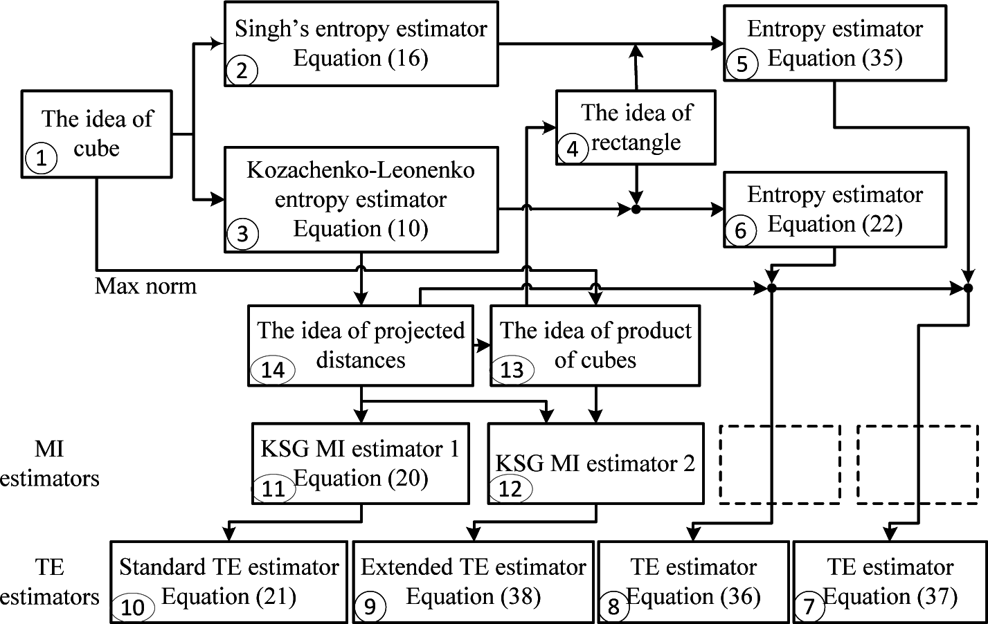
In what follows, when explaining the links among the existing methods and the proposed ones, we refer to Figure 1. In this diagram, a box identified by a number k in a circle is designed by box ⓚ.

Improving performance (in terms of bias and variance) of TE and MI estimators (obtained by choosing specific estimation functions $\widehat{\log (p(\cdot ))}$) in Equations (8) and (9), respectively) remains an issue when applied on short-length IID (or non-IID) sequences [3]. In this work, we particularly focused on bias reduction. For MI, the most widely-used estimator is the Kraskov–Stögbauer–Grassberger (KSG) estimator [24,31], which was later extended to estimate transfer entropy, resulting in the k-NN TE estimator [25–27,32–35] (adopted in the widely-used TRENTOOL open source toolbox, Version 3.0). Our contribution originated in the Kozachenko–Leonenko entropy estimator summarized in [24] and proposed beforehand in the literature to get an estimation $\widehat{\mathcal{H}\left(X\right)}$ of the entropy $\mathcal{H}\left(X\right)$ of a continuously-distributed random vector X, from a finite sequence of independent outcomes x_i, i = 1, …, N. This estimator, as well as another entropy estimator proposed by Singh et al. in [36] are briefly described in Section 2.1, before we introduce, in Section 4, our two new TE estimators based on both of them. In Section 2.2, Kraskov MI and standard TE estimators derived in literature from the Kozachenko–Leonenko entropy estimator are summarized, and the passage from a square to rectangular neighboring region to derive new entropy estimation is detailed in Section 3. Our methodology is depicted in Figure 1.

2. Original k-Nearest-Neighbors Strategies

2.1. Kozachenko–Leonenko and Singh’s Entropy Estimators for a Continuously-Distributed Random Vector

2.1.1. Notations

Let us consider a sequence x_i, i = 1, …, N in ${ℝ}^{d_X}$ (in our context, this sequence corresponds to an outcome of an IID sequence X₁, …, X_N, such that the common probability distribution will be equal to that of a given random vector X). The set of the k nearest neighbors of x_i in this sequence (except for x_i) and the distance between x_i and its k-th nearest neighbor are respectively denoted by ${\chi }_i^k$ and $d_{x_i,k}$. We denote ${\mathcal{D}}_{x_i}({\chi }_i^k)\subset {ℝ}^{d_X}$ a neighborhood of x_i in ${ℝ}^{d_X}$, which is the image of $(x_i,{\chi }_i^k)$ by a set valued map. For a given norm ║·║ on ${ℝ}^{d_X}$ (Euclidean norm, maximum norm, etc.), a standard construction $(x_i,{\chi }_i^k)\in {({ℝ}^{d_X})}^{k+1}\to {\mathcal{D}}_{x_i}({\chi }_i^k)\subset {ℝ}^{d_X}$ is the (hyper-)ball of radius equal to $d_{x_i,k}$, i.e., ${\mathcal{D}}_{x_i}({\chi }_i^k)=\{x:\Vert x-x_i\Vert \le d_{x_i,k}\}$ The (hyper-)volume (i.e., the Lebesgue measure) of ${\mathcal{D}}_{x_i}({\chi }_i^k)$ is then ${\upsilon }_i={\displaystyle {\int }_{{\mathcal{D}}_{x_i}({\chi }_i^k)}dx}$ (where $dx\triangleq d{\mu }^{d_X}(x)$).

2.1.2. Kozachenko–Leonenko Entropy Estimator

The Kozachenko–Leonenko entropy estimator is given by (Box ③ in Figure 1):

$${\widehat{\mathcal{H}\left(X\right)}}_{KL}=\psi (N)+\frac{1}{N}{\displaystyle \sum _{i=1}^N\log ({\upsilon }_i)-\psi (k)},$$

(10)

where v_i is the volume of ${\mathcal{D}}_{x_i}({\chi }_i^k)=\{x:\Vert x-x_i\Vert \le d_{x_i,k}\}$ computed with the maximum norm and $\psi (k)=\frac{{\mathrm{\Gamma }}^{\prime }(k)}{\mathrm{\Gamma }(k)}$ denotes the digamma function. Note that using Equation (10), entropy is measured in natural units (nats).

To come up with a concise presentation of this estimator, we give hereafter a summary of the different steps to get it starting from [24]. First, let us consider the distance $d_{x_i,k}$ between x_i and its k-th nearest neighbor (introduced above) as a realization of the random variable $D_{x_i,k}$, and let us denote by $q_{x_i,k}\left(x\right)$, x ∈ ℝ, the corresponding probability density function (conditioned by X_i = x_i). Secondly, let us consider the quantity $h^{x_i}(\epsilon )={\displaystyle {\int }_{\Vert u-x_i\Vert \le \epsilon /2}\mathrm{d}{P}_X}(u)$. This is the probability mass of the (hyper-)ball with radius equal to ε/2 and centered on x_i. This probability mass is approximately equal to:

$$h^{x_i}(\epsilon )\simeq p_X(x_i){\displaystyle {\int }_{\Vert \xi \Vert \le \epsilon /2}\mathrm{d}{\mu }^d(\xi )=p_X}(x_i)c_d{\epsilon }^d,$$

(11)

if the density function is approximately constant on the (hyper-)ball. The variable c_d is the volume of the unity radius d-dimensional (hyper-)ball in ℝ^d (c_d = 1 with maximum norm). Furthermore, it can be established (see [24] for details) that the expectation $E[\log (h^{X_i}(D_{X_i,k}))]$ where $h^{X_i}$ is the random variable associated with $h^{x_i}$, $D_{X_i,k}$ (which must not be confused with the notation ${\mathcal{D}}_{x_i}({\chi }_i^k)$ introduced previously) denotes the random distance between the k-th neighbor selected in the set of random vectors {X_k, 1 ≤ k ≤ N, k 6= i}, and the random point X_i is equal to ψ(k) − ψ(N) and does not depend on p_X (·). Equating it with $E[\log (p_X(X_i)c_d{D}_{X_i,k})]$ leads to:

$$\begin{array}{c}\psi (k)-\psi (N)\simeq E[\log (p_X(X_i))]+E[\log (c_d{D}_{X_i,k}^d)]\\ =-\mathcal{H}(X_i)+E[\log (V_i)]\end{array}$$

(12)

and:

$$\mathcal{H}(X_i)\simeq \psi (N)-\psi (k)+E[\log (c_d{D}_{X_i,k}^d)].$$

(13)

Finally, by using the law of large numbers, when N is large, we get:

$$\begin{array}{c}\mathcal{H}(X_i)\simeq \psi (N)-\psi (k)+\frac{1}{N}{\displaystyle \sum _{i=1}^N\log ({\upsilon }_i)}\\ =\widehat{\mathcal{H}{(X)}_{KL},}\end{array}$$

(14)

where v_i is the realization of the random (hyper-)volume $V_i=c_d{D}_{x_i,k}^d$.

Moreover, as observed in [24], it is possible to make the number of neighbors k depend on i by substituting the mean $\frac{1}{N}{\displaystyle {\sum }_{i=1}^N\psi (k_i)}$ for the constant ψ(k) in Equation (14), so that $\widehat{\mathcal{H}{(X)}_{KL}}$ becomes:

$$\widehat{\mathcal{H}{(X)}_{KL}}=\psi (N)+\frac{1}{N}{\displaystyle \sum _{i=1}^N(\log ({\upsilon }_i)-\psi (k_i))}.$$

(15)

2.1.3. Singh’s Entropy Estimator

The question of k-NN entropy estimation is also discussed by Singh et al. in [36], where another estimator, denoted by $\widehat{\mathcal{H}{(X)}_S}$ hereafter, is proposed (Box ② in Figure 1):

$$\widehat{\mathcal{H}{(X)}_S}=\log (N)+\frac{1}{N}{\displaystyle \sum _{i=1}^N\log ({\upsilon }_i)-\psi (k)}.$$

(16)

Using the approximation ψ(N) ≈ log(N) for large values of N, the estimator given by Equation (16) is close to that defined by Equation (10). This estimator was derived by Singh et al. in [36] through the four following steps:

• Introduce the classical entropy estimator structure:

  $$\widehat{\mathcal{H}(X)}\triangleq -\frac{1}{N}{\displaystyle \sum _{i=1}^N\log \widehat{p_X(X_i)}=\frac{1}{N}}{\displaystyle \sum _{i=1}^N{T}_i},$$

  (17)

  where:

  $$\widehat{p_X(X_i)}\triangleq \frac{k}{N{\upsilon }_i}.$$

  (18)
• Assuming that the random variables T_i, i = 1, …, N are identically distributed, so that $E[\widehat{\mathcal{H}(X)}]=E(T_1)$ (note that E(T₁) depends on N, even if the notation does not make that explicit), compute the asymptotic value of E(T₁) (when N is large) by firstly computing its asymptotic cumulative probability distribution function and the corresponding probability density $p_{T_1}$, and finally, compute the expectation $E(T_1)={\displaystyle {\int }_{ℝ}t{p}_{T_1}(t)\mathrm{d}t}$.
• It appears that $E(T_1)=E\left[\widehat{\mathcal{H}(X)}\right]=\mathcal{H}(X)+B$ where B is a constant, which is identified with the bias.
• Subtract this bias from $\widehat{\mathcal{H}(X)}$ to get ${\widehat{\mathcal{H}(X)}}_S=\widehat{\mathcal{H}(X)}-B$ and the formula given in Equation (16).

Note that the cancellation of the asymptotic bias does not imply that the bias obtained with a finite value of N is also exactly canceled. In Appendix C, we explain the origin of the bias for the entropy estimator given in Equation (17).

Observe also that, as for the Kozachenko–Leonenko estimator, it is possible to adapt Equation (16) if we want to consider a number of neighbors k_i depending on i. Equation (16) must then be replaced by:

$$\widehat{\mathcal{H}{(X)}_S}=\log (N)+\frac{1}{N}{\displaystyle \sum _{i=1}^N(\log ({\upsilon }_i)-\psi (k_i))}.$$

(19)

2.2. Standard Transfer Entropy Estimator

Estimating entropies separately in Equations (8) and (9) leads to individual bias values. Now, it is possible to cancel out (at least partially) the bias considering the algebraic sums (Equations (8) and (9)). To help in this cancellation, on the basis of Kozachenko–Leonenko entropy estimator, Kraskov et al. proposed to retain the same (hyper-)ball radius for each of the different spaces instead of using the same number k for both joint space ${\mathcal{S}}_{X,Y}$ and marginal spaces ( ${\mathcal{S}}_X$ and ${\mathcal{S}}_Y$ spaces) [24,37], leading to the following MI estimator (Box ⑪ in Figure 1):

$${\widehat{I}}_K=\psi (k)+\psi (N)-\frac{1}{N}{\displaystyle \sum _{i=1}^N[\psi (n_{X,i}+1)+\psi (n_{Y,i}+1)]},$$

(20)

where n_X,i and n_Y,i denote the number of points that strictly fall into the resulting distance in the lower-dimensional spaces ${\mathcal{S}}_X$ and ${\mathcal{S}}_Y$, respectively.

Applying the same strategy to estimate TE, the number of neighbors in the joint space ${\mathcal{S}}_{X^p,X^{-},Y^{-}}$S_X is first fixed, then for each i, the resulting distance ${\epsilon }_i\triangleq d_{(x_i^p,x_i^{-},y_i^{-}),k}$ is projected into the other three lower dimensional spaces, leading to the standard TE estimator [25,27,28] (implementation available in the TRENTOOL toolbox, Version 3.0, Box ⑩ in Figure 1):

$$\widehat{T{E}_{Y\to XSA}}=\psi (k)+\frac{1}{N}{\displaystyle \sum _{i=1}^N[\psi (n_{X^{-},i}+1)-\psi (n_{(X^{-},Y^{-}),i}+1)-\psi (n_{(X^p,X^{-}),i}+1)]},$$

(21)

where $n_{X^{-},i}$, $n_{(X^{-},Y^{-}),i}$, $n_{(X^p,X^{-}),i}$ denote the number of points that fall into the distance ε_i from $x_i^{-}$, $\left(x_i^{-},y_i^{-}\right)$ and $\left(x_i^p,x_i^{-}\right)$ in the lower dimensional spaces ${\mathcal{S}}_{X^{-}}$, ${\mathcal{S}}_{X^{-},Y^{-}}$ and $S_{X^p,X^{-}}$, respectively. This estimator is marked as the “standard algorithm” in the experimental part.

Note that a generalization of Equation (21) was proposed in [28] to extend this formula to the estimation of entropy combinations other than MI and TE.

3. From a Square to a Rectangular Neighboring Region for Entropy Estimation

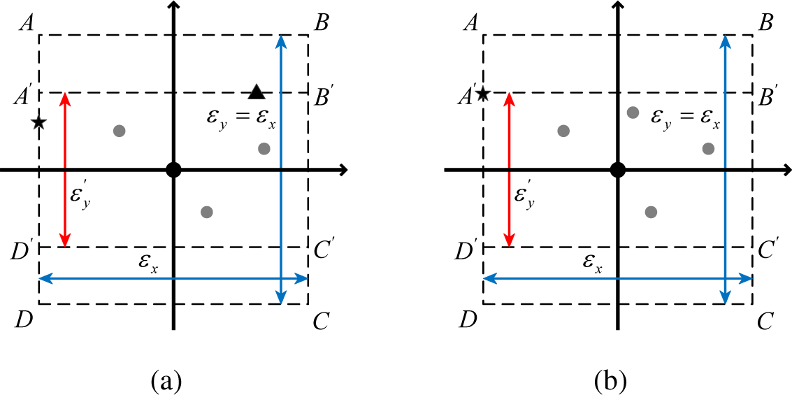
In [24], to estimate MI, as illustrated in Figure 2, Kraskov et al. discussed two different techniques to build the neighboring region to compute $\widehat{\mathcal{I}(X;Y)}$: in the standard technique (square ABCD in Figure 2a,b), the region determined by the first k nearest neighbors is a (hyper-)cube and leads to Equation (20), and in the second technique (rectangle A′B′C′D′ in Figure 2a,b), the region determined by the first k nearest neighbors is a (hyper-)rectangle. Note that the TE estimator mentioned in the previous section (Equation (21)) is based on the first situation (square ABCD in Figure 2a or 2b). The introduction of the second technique by Kraskov et al. was to circumvent the fact that Equation (15) was not applied rigorously to obtain the terms ψ(n_X,i+1) or ψ(n_Y,i+1) in Equation (20). As a matter of fact, for one of these terms, no point x_i (or y_i) falls exactly on the border of the (hyper-)cube ${\mathcal{D}}_{x_i}$ (or ${\mathcal{D}}_{y_i}$) obtained by the distance projection from the ${\mathcal{S}}_{X,Y}$ space. As clearly illustrated in Figure 2 (rectangle A′B′C′D′ in Figure 2a,b), the second strategy prevents that issue, since the border of the (hyper-)cube (in this case, an interval of ℝ) after projection from ${\mathcal{S}}_{X,Y}$ space to ${\mathcal{S}}_X$ space (or ${\mathcal{S}}_Y$ space) contains one point. When the dimensions of ${\mathcal{S}}_X$ and ${\mathcal{S}}_Y$ are larger than one, this strategy leads to building an (hyper-)rectangle equal to the product of two (hyper-)cubes, one of them in ${\mathcal{S}}_X$ and the other one in ${\mathcal{S}}_Y$. If the maximum distance of the k-th NN in ${\mathcal{S}}_{X,Y}$ is obtained in one of the directions in ${\mathcal{S}}_X$, this maximum distance, after multiplying by two, fixes the size of the (hyper-)cube in ${\mathcal{S}}_X$. To obtain the size of the second (hyper-)cube (in ${\mathcal{S}}_Y$), the k neighbors in ${\mathcal{S}}_{X,Y}$ are first projected on ${\mathcal{S}}_Y$, and then, the largest of the distances calculated from these projections fixes the size of this second (hyper-)cube.

In the remainder of this section, for an arbitrary dimension d, we propose to apply this strategy to estimate the entropy of a single multidimensional variable X observed in ℝ^d. This leads to introducing a d-dimensional (hyper-)rectangle centered on x_i having a minimal volume and including the set ${\chi }_i^k$ of neighbors. Hence, the rectangular neighboring is built by adjusting its size separately in each direction in the space ${\mathcal{S}}_X$. Using this strategy, we are sure that, in any of the d directions, there is at least one point on one of the two borders (and only one with probability one). Therefore, in this approach, the (hyper-)rectangle, denoted by $D_{x_i}^{{\epsilon }_1,\dots ,{\epsilon }_d}$, where the sizes ε₁, …, ε_d in the respective d directions are completely specified from the neighbors set ${\chi }_i^k$, is substituted for the basic (hyper-)square ${\mathcal{D}}_{x_i}({\chi }_i^k)=\{:\Vert x-x_i\Vert \le d_{x_i,k}\}$. It should be mentioned that the central symmetry of the (hyper-)rectangle around the center point allows for reducing the bias in the density estimation [38] (cf. Equation (11) or (18)). Note that, when k < d, there must exist neighbors positioned on some vertex or edges of the (hyper-)rectangle. With k < d, it is impossible that, for any direction, one point falls exactly inside a face (i.e., not on its border). For example, with k = 1 and d > 1, the first neighbor will be on a vertex, and the sizes of the edges of the reduced (hyper-)rectangle will be equal to twice the absolute value of its coordinates, whatever the direction.

Hereafter, we propose to extend the entropy estimators by Kozachenko–Leonenko and Singh using the above strategy before deriving the corresponding TE estimators and comparing their performance.

3.1. Extension of the Kozachenko–Leonenko Method

As indicated before, in [24], Kraskov et al. extended the Kozachenko–Leonenko estimator (Equations (10) and (15)) using the rectangular neighboring strategy to derive the MI estimator. Now, focusing on entropy estimation, after some mathematical developments (see Appendix D), we obtain another estimator of $\mathcal{H}(X)$, denoted by ${\widehat{\mathcal{H}(X)}}_K$ (Box ⑥ in Figure 1),

$${\widehat{\mathcal{H}(X)}}_K=\psi (N)+\frac{1}{N}{\displaystyle \sum _{i=1}^N\log ({\upsilon }_i)-\psi (k)}+\frac{d-1}{k}.$$

(22)

Here, v_i is the volume of the minimum volume (hyper-)rectangle around the point x_i. Exploiting this entropy estimator, after substitution in Equation (8), we can derive a new estimation of TE.

3.2. Extension of Singh’s Method

We propose in this section to extend Singh’s entropy estimator by using a (hyper-)rectangular domain, as we did for the Kozachenko–Leonenko estimator extension introduced in the preceding section. Considering a d-dimensional random vector X ∈ ℝ^d continuously distributed according to a probability density function p_X, we aim at estimating the entropy $\mathscr{H}$(X) from the observation of a p_X distributed IID random sequence X_i, i = 1, …, N. For any specific data point x_i and a fixed number k (1 ≤ k ≤ N), the minimum (hyper-)rectangle (rectangle A′B′C′D′ in Figure 2) is fixed, and we denote this region by $D_{x_i}^{{\epsilon }_1,\dots ,{\epsilon }_d}$ and its volume by v_i. Let us denote ξ_i (1 ≤ ξ_i ≤ min(k, d)) the number of points on the border of the (hyper-)rectangle that we consider as a realization of a random variable Ξ_i. In the situation described in Figure 2a,b, ξ_i = 2 and ξ_i = 1, respectively. According to [39] (Chapter 6, page 269), if ${\mathcal{D}}_{x_i}({\chi }_i^k)$ corresponds to a ball (for a given norm) of volume v_i, an unbiased estimator of p_X(x_i) is given by:

$$\widehat{p_X(x_i)}=\frac{k-1}{N{\upsilon }_i},i=1,2,\dots ,N.$$

(23)

This implies that the classical estimator $\widehat{p_X(x_i)}=\frac{k}{N{\upsilon }_i}$ is biased and that presumably $\log (\frac{k}{N{\upsilon }_i})$ is also a biased estimation of (p_X(x_i)) for N large, as shown in [39].

Now, in the case ${\mathcal{D}}_{x_i}({\chi }_i^k)$, is the minimal (i.e., with minimal (hyper-)volume) (hyper-)rectangle $D_{x_i}^{{\epsilon }_1,\dots ,{\epsilon }_d}$, including ${\chi }_i^k$, more than one point can belong to the border, and a more general estimator $\widetilde{p_X(x_i)}$ of p_X(x_i) can be a priori considered:

$$\widetilde{p_X(x_i)}=\frac{{\tilde{k}}_i}{N{\upsilon }_i},$$

(24)

where ${\tilde{k}}_i$ is some given function of k and ξ_i. The corresponding estimation of $\mathcal{H}(X)$ is then:

$$\widehat{\mathcal{H}(X)}=-\frac{1}{N}{\displaystyle \sum _{i=1}^N\log }\widetilde{(p_X(x_i}))=\frac{1}{N}{\displaystyle \sum _{i=1}^N{t}_i},$$

(25)

with:

$$t_i=\log \left(\frac{N{\upsilon }_i}{{\tilde{k}}_i}\right),i=1,2,\dots ,N,$$

(26)

t_i being realizations of random variables T_i and ${\tilde{k}}_i$ being realizations of random variables ${\tilde{K}}_i$. We have:

$$\forall i=1,\dots ,N:E\left[\widehat{\mathcal{H}(X)}\right]=E(T_i)=E(T_1).$$

(27)

Our goal is to derive $E\left[\widehat{\mathcal{H}(X)}\right]-\mathcal{H}(X)=E(T_1)-\mathcal{H}(X)$ for N large to correct the asymptotic bias of $\widehat{\mathcal{H}(X)}$, according to Steps (1) to (3), explained in Section 2.1.3. To this end, we must consider an asymptotic approximation of the conditional probability distribution $\mathcal{P}(T_1\le r|X_1=x_1,{\mathrm{\Xi }}_1={\xi }_1)$ before computing the asymptotic difference between the expectation E [T₁] = E [E [T₁|X₁ = x₁, Ξ₁ = ξ₁]] and the true entropy $\mathcal{H}(X)$.

Let us consider the random Lebesgue measure V₁ of the random minimal (hyper-)rectangle $D_{x_1}^{{\epsilon }_1,\dots ,{\epsilon }_d}$ ((ϵ₁, …, ϵ_d) denotes the random vector for which (ε₁, …, ε_d) ∈ ℝ^d is a realization) and the relation $T_1=\log \left(\frac{N{V}_1}{{\tilde{K}}_1}\right)$. For any r > 0, we have:

$$\begin{array}{c}\mathcal{P}(T_1>r|X_1=x_1,{\mathrm{\Xi }}_1={\xi }_1)=\mathcal{P}\left(\log \left(\frac{N{V}_1}{{\tilde{K}}_1}\right)>r|X_1=x_1,{\mathrm{\Xi }}_1={\xi }_1\right)\\ =\mathcal{P}(V_1>{\upsilon }_r|X_1=x_1,{\mathrm{\Xi }}_1={\xi }_1),\end{array}$$

(28)

where ${\upsilon }_r=e^r\frac{{\tilde{k}}_1}{N}$, since, conditionally to Ξ₁ = ξ₁, we have ${\tilde{K}}_1={\tilde{k}}_1$.

In Appendix E, we prove the following property.

Property 1. For N large,

$$\mathcal{P}(T_1>r|X_1=x_1,{\mathrm{\Xi }}_1={\xi }_1)\simeq {\displaystyle \sum _{i=0}^{k-{\xi }_1}\left(\begin{array}{c}N-{\xi }_1-1\\ i\end{array}\right)}{(p_X(x_1){\upsilon }_r)}^i{(1-p_X(x_1){\upsilon }_r)}^{N-{\xi }_1-1-i}.$$

(29)

The Poisson approximation (when N → ∞ and v_r → 0) of the binomial distribution summed in Equation (29) leads to a parameter λ = (N − ξ₁ − 1) p_X(x₁)v_r. As N is large compared to ξ₁ + 1, we obtain from Equation (26):

$$\mathrm{\lambda }\simeq {\tilde{k}}_1{e}^r{p}_X(x_1),$$

(30)

and we get the approximation:

$$\underset{N\to \infty }{\lim }\mathcal{P}(T_1>r|X_1=x_1,{\mathrm{\Xi }}_1={\xi }_1)\simeq {\displaystyle \sum _{i=0}^{k-{\xi }_1}\frac{{\left[{\tilde{k}}_1{e}^r{p}_X(x_1)\right]}^i}{i!}}{e}^{-{\tilde{k}}_1{e}^r{p}_X(x_1)}.$$

(31)

Since $\mathcal{P}(T_1\le r|X_1=x_1,{\mathrm{\Xi }}_1={\xi }_1)=1-\mathcal{P}(T_1>r|X_1=x_1,{\mathrm{\Xi }}_1={\xi }_1)$, we can get the density function of T₁, noted $g_{T_1}(r)$, by deriving $\mathcal{P}(T_1\le r|X_1=x_1,{\mathrm{\Xi }}_1={\xi }_1)$. After some mathematical developments (see Appendix F), we obtain:

$$\begin{array}{cc}\begin{array}{c}{g}_{T_1}\left(r\right)={\mathcal{P}}^{\prime }(T_1\le r|X_1=x_1,{\mathrm{\Xi }}_1={\xi }_1)\\ =-{\mathcal{P}}^{\prime }(T_1>r|X_1=x_1,{\mathrm{\Xi }}_1={\xi }_1)\\ =\frac{{\left[{\tilde{k}}_1{e}^r{p}_X(x_1)\right]}^{(k-{\xi }_1+1)}}{(k-{\xi }_1)!}{e}^{-{\tilde{k}}_1{e}^r{p}_X(x_1)}\end{array}& ,r\in ℝ\end{array},$$

(32)

and consequently (see Appendix G for details),

$$\begin{array}{r}\underset{N\to \infty }{\lim }E[T_1|X_1=x_1,{\mathrm{\Xi }}_1={\xi }_1]={\displaystyle {\int }_{-\infty }^{\infty }\frac{{\left[{\tilde{k}}_1{e}^r{p}_X(x_1)\right]}^{(k-{\xi }_1+1)}}{(k-{\xi }_1)!}{e}^{-{\tilde{k}}_1{e}^r{p}_X(x_1)}\mathrm{d}r}\\ =\psi (k-{\xi }_1+1)-\log ({\tilde{k}}_1)-\log (p_X(x_1)).\end{array}$$

(33)

Therefore, with the definition of differential entropy $\mathscr{H}$(X₁) = E[−log (p_X(X₁))], we have:

$$\underset{N\to \infty }{\lim }E[T_1]=\underset{N\to \infty }{\lim }E[E[T_1|X_1,{\mathrm{\Xi }}_1]]=E\left[\psi (k-{\mathrm{\Xi }}_1+1)-\log ({\tilde{K}}_1)\right]+\mathcal{H}(X_1).$$

(34)

Thus, the estimator expressed by Equation (25) is asymptotically biased. Therefore, we consider a modified version, denoted by ${\widehat{\mathcal{H}(X)}}_{NS}$, obtained by subtracting an estimation of the bias $E\left[\psi (k-{\mathrm{\Xi }}_1+1)-\log ({\tilde{K}}_1)\right]$ given by the empirical mean $\frac{1}{N}{\displaystyle {\sum }_{i=1}^N\psi (k-{\xi }_i+1)}\frac{1}{N}{\displaystyle {\sum }_{i=1}^N\log ({\tilde{k}}_i)}$ (according to the large numbers law), and we obtain, finally (Box ⑤ in Figure 1):

$$\begin{array}{l}{\widehat{\mathcal{H}(X)}}_{NS}=\frac{1}{N}{\displaystyle \sum _{i=1}^N{t}_i}-\frac{1}{N}{\displaystyle \sum _{i=1}^N\psi (k-{\xi }_i+1)}+\frac{1}{N}{\displaystyle \sum _{i=1}^N\log ({\tilde{k}}_i)}\\ =\frac{1}{N}{\displaystyle \sum _{i=1}^N\log \left(\frac{N{\upsilon }_i}{{\tilde{k}}_i}\right)}-\frac{1}{N}{\displaystyle \sum _{i=1}^N\psi (k-{\xi }_i+1)}+\frac{1}{N}{\displaystyle \sum _{i=1}^N\log ({\tilde{k}}_i)}\\ =\log (N)+\frac{1}{N}{\displaystyle \sum _{i=1}^N\log ({\upsilon }_i)}-\frac{1}{N}{\displaystyle \sum _{i=1}^N\psi (k-{\xi }_i+1)}.\end{array}$$

(35)

In comparison with the development of Equation (22), we followed here the same methodology, except we take into account (through a conditioning technique) the influence of the number of points on the border.

We observe that, after cancellation of the asymptotic bias, the choice of the function of k and ξ_i to define ${\tilde{k}}_i$ in Equation (24) does not have any influence on the final result. In this way, we obtain an expression for ${\widehat{\mathcal{H}(X)}}_{NS}$, which simply takes into account the values ξ_i that could a priori influence the entropy estimation.

Note that, as for the original Kozachenko–Leonenko (Equation (10)) and Singh (Equation (16)) entropy estimators, both new estimation functions (Equation (22) and (35)) hold for any value of k, such that k ≪ N, and we do not have to choose a fixed k while estimating entropy in lower dimensional spaces. Therefore, under the framework proposed in [24], we built two different TE estimators using Equations (22) and (35), respectively.

3.3. Computation of the Border Points Number and of the (Hyper-)Rectangle Sizes

We explain more precisely hereafter how to determine the numbers of points ξ_i on the border. Let us denote $x_i^j\in {ℝ}^d$ j = 1,…, k, the k nearest neighbors of $x_i\in {ℝ}^d$, and let us consider the d × k array D_i, such that for any (p, j) ∈ {1, …, d} × {1,…, k}, $D_i(p,j)=\left|x_i^j(p)-x_i(p)\right|$ is the distance (in R) between the p-th component $x_i^j(p)$ of $x_i^j$ and the p-th component x_i(p) of x_i. For each p, let us introduce J_i(p) ∈ {1, …, k} defined by D_i(p, J_i(p)) = max (D_i(p, 1), …, D_i(p, k)) and which is the value of the column index of D_i for which the distance D_i(p, j) is maximum in the row number p. Now, if there exists more than one index J_i(p) that fulfills this equality, we select arbitrarily the lowest one, hence avoiding the max(·) function to be multi-valued. The MATLAB implementation of the max function selects such a unique index value. Then, let us introduce the d × k Boolean array B_i defined by B_i(p, j) = 1 if j = J_i(p) and B_i(p, j) = 0, otherwise. Then:

• The d sizes ε_p, p = 1, …, d of the (hyper-)rectangle $D_{x_i}^{{\epsilon }_1,\dots ,{\epsilon }_d}$ xi are equal respectively to ε_p = 2D_i(p, J_i(p)), p = 1, …, d.
• We can define ξ_i as the number of non-null column vectors in B_i. For example, if the k-th nearest neighbor $x_i^k$ is such that ∀j ≠ k, $\forall p=1,\dots ,d:\left|x_i^j(p)-x_i(p)\right|<\left|x_i^k(p)-x_i(p)\right|$ i.e., when the k-th nearest neighbor is systematically the farthest from the central point x_i for each of the d entries directions, then all of the entries in the last column of B_i are equal to one, while all other are equal to zero: we have only one column including values different from zero and, so, only one point on the border (ξ_i = 1), which generalizes the case depicted in Figure 2b for d = 2.

N.B.: this determination of ξ_i may be incorrect when there exists a direction p, such that the number of indices j for which D_i(p, j) reaches the maximal value is larger than one: the value of ξ_i obtained with our procedure can then be underestimated. However, we can argue that, theoretically, this case occurs with a probability equal to zero (because the observations are continuously distributed in the probability) and, so, it can be a priori discarded. Now, in practice, the measured quantification errors and the round off errors are unavoidable, and this probability will differ from zero (although remaining small when the aforesaid errors are small): theoretically distinct values D_i(p, j) on the row p of D_i may be erroneously confounded after quantification and rounding. However, the max(·) function then selects on row p only one value for J_i(p) and, so, acts as an error correcting procedure. The fact that the maximum distance in the concerned p directions can then be allocated to the wrong neighbor index has no consequence for the correct determination of ξ_i.

4. New Estimators of Transfer Entropy

From an observed realization $\left(x_i^p,x_i^{-},y_i^{-}\right)\in {\mathcal{S}}_{X^p,X^{-},Y^{-}}$, i = 1, 2, …, N of the IID random sequence $\left(X_i^p,X_i^{-},Y_i^{-}\right)$, i = 1, 2, …, N and a number k of neighbors, the procedure could be summarized as follows (distances are from the maximum norm):

• similarly to the MILCA [31] and TRENTOOL toolboxes [34], normalize, for each i, the vectors $x_i^p$, $x_i^{-}$ and $y_i^{-}$;
• in joint space ${\mathcal{S}}_{X^p,X^{-},Y^{-}}$, for each point $\left(x_i^p,x_i^{-},y_i^{-}\right)$, calculate the distance $d_{\left(x_i^p,x_i^{-},y_i^{-}\right),k}$ between $\left(x_i^p,x_i^{-},y_i^{-}\right)$ and its k-th neighbor, then construct the (hyper-)rectangle with sizes ε₁, …, ε_d (d is the dimension of the vectors $\left(x_i^p,x_i^{-},y_i^{-}\right)$), for which the (hyper-)volume is ${\upsilon }_{(X^p,X^{-},Y^{-}),i}{\epsilon }_1\times \dots \times {\epsilon }_d$ and the border contains ${\xi }_{(X^p,X^{-},Y^{-}),i}$ points;
• for each point $\left(x_i^p,x_i^{-}\right)$ in subspace ${\mathcal{S}}_{X^p,X^{-}}$, count the number $k_{(X^p,X^{-}),i}$ of points falling within the distance $d_{\left(x_i^p,x_i^{-},y_i^{-}\right),k}$, then find the smallest (hyper-)rectangle that contains all of these points and for which ${\upsilon }_{(X^p,X^{-}),i}$ and ${\xi }_{(X^p,X^{-}),i}$ are respectively the volume and the number of points on the border; repeat the same procedure in subspaces ${\mathcal{S}}_{X^{-},Y^{-}}$ and ${\mathcal{S}}_{X^{-}}$.

From Equation (22) (modified to k not constant for ${\mathcal{S}}_{X^{-}}$, ${\mathcal{S}}_{X^p,X^{-}}$ and ${\mathcal{S}}_{X^{-},Y^{-}}$), the final TE estimator can be written as (Box ⑧ in Figure 1):

$$\begin{array}{l}\widehat{T{E}_{Y\to X_{p}1}}=\frac{1}{N}{\displaystyle \sum _{i=1}^N\log }\frac{{\upsilon }_{(X^p,X^{-}),i}\cdot {\upsilon }_{(X^{-},Y^{-}),i}}{{\upsilon }_{(X^p,X^{-},Y^{-}),i}\cdot {\upsilon }_{X^{-},i}}\\ +\frac{1}{N}{\displaystyle \sum _{i=1}^N(\psi (k)+\psi (k_{X^{-},i})-\psi (k_{(X^p,X^{-}),i})-\psi (k_{(X^{-},Y^{-}),i})}\\ +\frac{d_{X^p}+d_{X^{-}}-1}{k_{(X^p,X^{-}),i}}+\frac{d_{X^{-}}+d_{Y^{-}}-1}{k_{(X^{-},Y^{-}),i}}-\frac{d_{X^p}+d_{X^{-}}+d_{Y^{-}}-1}{k}-\frac{d_{X^{-}}-1}{k_{X^{-},i}}),\end{array}$$

(36)

where $d_{X^p}=\dim ({\mathcal{S}}_{X^p})$, $d_{X^{-}}=\dim ({\mathcal{S}}_{X^{-}})$, $d_{Y^{-}}=\dim ({\mathcal{S}}_{Y^{-}})$, and with Equation (35), it yields to (Box ⑦ in Figure 1):

$$\begin{array}{l}\widehat{T{E}_{Y\to X_{p}2}}=\frac{1}{N}{\displaystyle \sum _{i=1}^N\log }\frac{{\upsilon }_{(X^p,X^{-}),i}\cdot {\upsilon }_{(X^{-},Y^{-}),i}}{{\upsilon }_{(X^p,X^{-},Y^{-}),i}\cdot {\upsilon }_{X^{-},i}}\\ +\frac{1}{N}{\displaystyle \sum _{i=1}^N(\psi (k-{\xi }_{(X^p,X^{-},Y^{-}),i}+1)+\psi (k_{X^{-},i}-{\xi }_{X^{-},i}+1)-\psi (k_{(X^p,X^{-}),i}}\\ -{\xi }_{(X^p,X^{-}),i}+1)+\psi (k_{(X^{-},Y^{-}),i}-{\xi }_{(X^{-},Y^{-}),i}+1)).\end{array}$$

(37)

In Equations (36) and (37), the volumes ${\upsilon }_{(X^p,X^{-}),i}$, ${\upsilon }_{\left(X^{-},Y^{-}\right),i}$, ${\upsilon }_{(X^p,X^{-},Y^{-}),i}$, ${\upsilon }_{X^{-},i}$ are obtained by computing, for each of them, the product of the edges lengths of the (hyper-)rectangle, i.e., the product of d edges lengths, d being respectively equal to $d_{X^p}+d_{X^{-}}$, $d_{X^{-}}+d_{Y^{-}}$, $d_{X^p}+d_{X^{-}}+d_{Y^{-}}$ and $d_{X^{-}}$. In a given subspace and for a given direction, the edge length is equal to twice the largest distance between the corresponding coordinate of the reference point (at the center) and each of the corresponding coordinates of the k nearest neighbors. Hence a generic formula is ${\upsilon }_U={\displaystyle {\prod }_{j=1}^{\dim (\mathcal{U})}{\epsilon }_{Uj}}$, where U is one of the symbols (X^p, X⁻), (X⁻, Y⁻), (X^p, X⁻, Y⁻) and X⁻ and the ε_Uj are the edge lengths of the (hyper-)rectangle.

The new TE estimator $\widehat{{\mathrm{TE}}_{Y\to X_{p}1}}$ (Box ⑧ in Figure 1) can be compared with the extension of $\widehat{{\mathrm{TE}}_{Y\to XSA}}$, the TE estimator proposed in [27] (implemented in the JIDT toolbox [30]). This extension [27], included in Figure 1 (Box ⑨), is denoted here by $\widehat{{\mathrm{TE}}_{Y\to XEA}}$. The main difference with our $\widehat{{\mathrm{TE}}_{Y\to X_{p}1}}$ estimator is that our algorithm uses a different length for each sub-dimension within a variable, rather than one length for all sub-dimensions within the variable (which is the approach of the extended algorithm). We introduced this approach to make the tightest possible (hyper-)rectangle around the k nearest neighbors. $\widehat{{\mathrm{TE}}_{Y\to XEA}}$ is expressed as follows:

$$\begin{array}{l}\widehat{{\mathrm{TE}}_{Y\to XEA}}=\frac{1}{N}{\displaystyle \sum _{i=1}^N(\psi (k)-\frac{2}{k}+\psi (l_{X^{-},i})-\psi (l_{(X^{-},X^{-}),i})}\\ +\frac{1}{l_{(X^p,X^{-}),i}}-\psi (l_{(X^{-},Y^{-}),i})+\frac{1}{l_{(X^{-},Y^{-}),i}}).\end{array}$$

(38)

In the experimental part, this estimator is marked as the “extended algorithm”. It differs from Equation (36) in two ways. Firstly, the first summation on the right hand-side of Equation (36) does not exist. Secondly, compared with Equation (36), the numbers of neighbors $k_{X^{-},i}$, $k_{(X^p,X^{-}),i}$ and $k_{(X^{-},Y^{-}),i}$ included in the rectangular boxes, as explained in Section 3.1, are replaced respectively with $l_{X^{-},i}$, $l_{(X^p,X^{-}),i}$ and $l_{(X^{-},Y^{-}),i}$, which are obtained differently. More precisely, Step (2) in the above algorithm becomes:

• (2′) For each point $(x_i^p,x_i^{-})$ in subspace ${\mathcal{S}}_{X^p,X^{-}}$, $l_{(X^p,X^{-}),i}$ is the number of points falling within a (hyper-)rectangle equal to the Cartesian product of two (hyper-)cubes, the first one in ${\mathcal{S}}_{X^p}$ and the second one in ${\mathcal{S}}_{X^{-}}$, whose edge lengths are equal, respectively, to $d_{x_i^p}^{\max }=2\times \max \left\{\Vert x_k^p-x_i^p\Vert :{(x^p,x^{-},y^{-})}_k\in {\chi }_{(x^p,x^{-},y^{-})i}^k\right\}$ and $d_{x_i^{-}}^{\max }=2\times \max \left\{\Vert x_k^{-}-x_i^{-}\Vert :{(x^p,x^{-},y^{-})}_k\in {\chi }_{(x^p,x^{-},y^{-})i}^k\right\}$, i.e., $l_{(X^p,X^{-}),i}=card\left\{(x_j^p,x_i^{-}):j\in \{\{1,\dots ,N\}-\{i\}\}\&\Vert x_j^p,x_i^p\Vert \le d_{x_i^p}^{\max }\&\Vert x_j^{-},x_i^{-}\Vert \le d_{x_i^{-}}^{\max }\right\}$. Denote by ${\upsilon }_{(X^p,X^{-}),i}$ the volume of this (hyper-)rectangle. Repeat the same procedure in subspaces ${\mathcal{S}}_{X^{-},Y^{-}}$ and ${\mathcal{S}}_{X^{-}}$.

Note that the important difference between the construction of the neighborhoods used in $\widehat{{\mathrm{TE}}_{Y\to XEA}}$ and is $\widehat{{\mathrm{TE}}_{Y\to X_{p}1}}$ is that, for the first case, the minimum neighborhood, including the k neighbors, is constrained to be a Cartesian product of (hyper-)cubes and, in the second case, this neighborhood is a (hyper-)rectangle whose edge lengths can be completely different.

5. Experimental Results

In the experiments, we tested both Gaussian IID and Gaussian AR models to compare and validate the performance of the TE estimators proposed in the previous section. For a complete comparison, beyond the theoretical value of TE, we also computed the Granger causality index as a reference (as indicated previously, in the case of Gaussian signals TE and Granger causality index are equivalent up to a factor of two; see Appendix H). In each following figure, GCi/2 corresponds to the Granger causality index divided by two; TE estimated by the free TRENTOOL toolbox (corresponding to Equation (21)) is marked as the standard algorithm; that estimated by JIDT (corresponding to Equation (38)) is marked as the extended algorithm; TE_p1 is the TE estimator given by Equation (36); and TE_p2 is the TE estimator given by Equation (37). For all of the following results, the statistical means and the standard deviations of the different estimators have been estimated using an averaging on 200 trials.

5.1. Gaussian IID Random Processes

The first model we tested, named Model 1, is formulated as follows:

$$X_t=a{Y}_t+b{Z}_t+W_t,W_t\in ℝ,Y\in {ℝ}^{d_Y},Z\in {ℝ}^{d_Y},$$

(39)

where $Y_t~\mathcal{N}(0,C_Y)$, $Z_t~\mathcal{N}(0,C_Z)$, $W_t~\mathcal{N}(0,{\sigma }_W^2)$, the three processes Y, Z, and W being mutually independent. The triplet (X_t, Y_t, Z_t) corresponds to the triplet $\left(X_i^p,X_i^{-},Y_i^{-}\right)$ introduced previously. C_U is a Toeplitz matrix with the first line equal to $[1,\alpha ,\dots ,{\alpha }^{d_U-1}]$. For the matrix C_Y, we chose α = 0.5, and for C_Z, α = 0.2. The standard deviation σ_W was set to 0.5. The vectors a and b were such that a = 0.1 ∗ [1, 2, …, d_Y] and b = 0.1 ∗ [d_Z, d_Z − 1, …, 1]. With this model, we aimed at estimating $\mathcal{H}\left(X|Y\right)-\mathcal{H}\left(X|Y,Z\right)$ to test if the knowledge of signals Y and Z could improve the prediction of X compared to only the knowledge of Y.

Results are reported in Figure 3 where the dimensions d_Y and d_Z are identical. We observe that, for a low dimension and a sufficient number of neighbors (Figure 3a), all TE estimators tend all the more to the theoretical value (around 0.26) that the length of the signals is large, the best estimation being obtained by the two new estimators. Compared to Granger causality, these estimators display a greater bias, but a lower variance. Due to the “curse of dimensionality”, with an increasing dimension (see Figure 3b), it becomes much more difficult to obtain an accurate estimation of TE. For a high dimension, all estimators reveal a non-negligible bias, even if the two new estimators still behave better than the two reference ones (standard and extended algorithms).

5.2. Vectorial AR Models

In the second experiment, two AR models integrating either two or three signals have been tested. The first vectorial AR model (named Model 2) we tested was as follows:

$$\{\begin{array}{l}{x}_t=0.45\sqrt{2}{x}_{t-1}-0.9x_{t-2}-0.6y_{t-2}+e_{x,t}\\ y_t=0.6x_{t-2}-0.175\sqrt{2}{y}_{t-1}+0.55\sqrt{2}{y}_{t-2}+e_{y,t}.\end{array}$$

(40)

The second vectorial AR model (named Model 3) was given by:

$$\{\begin{array}{l}{x}_t=-0.25x_{t-2}-0.35y_{t-2}+0.35z_{t-2}+e_{x,t}\\ y_t=-0.5x_{t-1}+0.25y_{t-1}-0.5z_{t-3}+e_{y,t}\\ z_t=-0.6x_{t-2}-0.7y_{t-2}-0.2z_{t-2}+e_{z,t}.\end{array}$$

(41)

For both models, e_x, e_y and e_z denote realizations of independent white Gaussian noises with zero mean and a variance of 0.1. As previously, we display in the following figures not only the theoretical value of TE, but also the Granger causality index for comparison. In this experiment, the prediction orders m and n were equal to the corresponding regression orders of the AR models. For example, when estimating TE_{Y → X}, we set m = 2, n = 2, and $\left(X_i^p,X_i^{-},Y_i^{-}\right)$ corresponds to $\left(X_{i+1},X_i^{(2)},Y_i^{(2)}\right)$.

For Figures 4 and 5, the number k of neighbors was fixed to eight, whereas, in Figure 6, this number was set to four and three (respectively Figures 6a,b) to show the influence of this parameter. Figures 4 and 6 are related to Model 2, and Figure 5 is related to Model 3.

As previously, for large values of k (cf. Figures 4 and 5), we observe that the four TE estimators converge towards the theoretical value. This result is all the more true when the signal length increases. As expected in such linear models, Granger causality outperforms the TE estimators at the expense of a slightly larger variance. Contrary to Granger causality, TE estimators are clearly more impacted by the signal length, even if their standard deviations remain lower. Here, again, when comparing the different TE estimators, it appears that the two new estimators achieve improved behavior compared to the standard and extended algorithms for large k.

In the scope of k-NN algorithms, the choice of k must be a tradeoff between the estimation of bias and variance. Globally, when the value of k decreases, the bias decreases for the standard and extended algorithms and for the new estimator TE_p1. Now, for the second proposed estimator TE_p2, it is much more sensitive to the number of neighbors (as can be seen when comparing Figures 4 and 6). As shown in Figures 3 and 5, the results obtained using TE_p2 and TE_p1 are quite comparable when the value of k is large (k = 8). Now, when the number of neighbors decreases, the second estimator we proposed, TE_p2, is much less reliable than all of the other ones (Figure 6). Concerning the variance, it remains relatively stable when the number of neighbors falls from eight to three, and in this case, the extended algorithm, which displays a slightly lower bias, may be preferred.

When using k = 8, a possible interpretation of getting a lower bias with our algorithms could be that, once we are looking at a large enough number of k nearest neighbors, there is enough opportunity for the use of different lengths on the sub-dimensions of the (hyper-)rectangle to make a difference to the results, whereas with k = 3, there is less opportunity.

To investigate the impact on the dispersion (estimation error standard deviation) of (i) the estimation method and (ii) the number of neighbors, we display in Figures 7a,b the boxplots of the absolute values of the centered estimation errors (AVCE) corresponding to experiments reported in Figures 4a and 6b for a 1024-point signal length. These results show that neither the value of k, nor the tested TE estimator dramatically influence the dispersions. More precisely, we used a hypothesis testing procedure (two-sample Kolmogorov–Smirnov goodness-of-fit hypothesis, KSTEST2 in MATLAB) to test if two samples (each with 200 trials) of AVCE are drawn from the same underlying continuous population or not. The tested hypothesis corresponds to non-identical distributions and is denoted H = 1, and H = 0 corresponds to the rejection of this hypothesis. The confidence level was set to 0.05.

• Influence of the method:

  • Test between the standard algorithm and TE_p1 in Figure 7a: H = 0, p-value = 0.69 → no influence
  • Test between the extended algorithm and TE_p1 in Figure 7a: H = 0, p-value = 0.91 → no influence
  • Test between the standard algorithm and TE_p1 in Figure 7b: H = 0, p-value = 0.081 → no influence
  • Test between the extended algorithm and TE_p1 in Figure 7b: H = 1, p-value = 0.018 → influence exists.
• Influence of the neighbors’ number k:

  • Test between k = 8 (Figure 7a) and k = 3 (Figure 7b) for the standard algorithm: H = 0, p-value = 0.97 → no influence
  • Test between k = 8 (Figure 7a) and k = 3 (Figure 7b) for TE_p1: H = 0, p-value = 0.97 → no influence.

For these six tested cases, the only case where a difference between distributions (and so, between the dispersions) corresponds to a different distribution is when comparing the extended algorithm and TE_p1 in Figure 7b.

6. Discussion and Summary

In the computation of k-NN based estimators, the most time-consuming part is the procedure of nearest neighbor searching. Compared to Equations (10) and (16), Equations (22) and (35) involve supplementary information, such as the maximum distance of the first k-th nearest neighbor in each dimension and the number of points on the border. However, most currently used neighbor searching algorithms, such as k-d tree (k-dimensional tree) and ATRIA (A TRiangle Inequality based Algorithm) [40], provide not only information on the k-th neighbor, but also on the first (k − 1) nearest neighbors. Therefore, in terms of computation cost, there is no significant difference among the three TE estimators (Boxes ⑦, ⑧, ⑨, ⑩ in Figure 1).

In this contribution, we discussed TE estimation based on k-NN techniques. The estimation of TE is always an important issue, especially in neuroscience, where getting large amounts of stationary data is problematic. The widely-used k-NN technique has been proven to be a good choice for the estimation of information theoretical measurement. In this work, we first investigated the estimation of Shannon entropy based on the k-NN technique involving a rectangular neighboring region and introduced two different k-NN entropy estimators. We derived mathematically these new entropy estimators by extending the results and methodology developed in [24] and [36]. 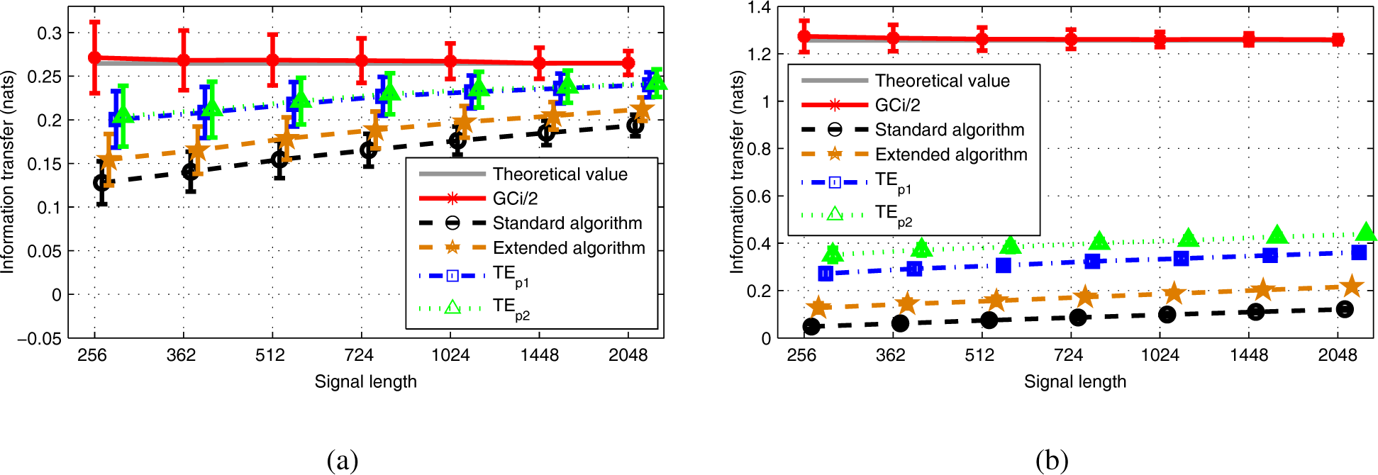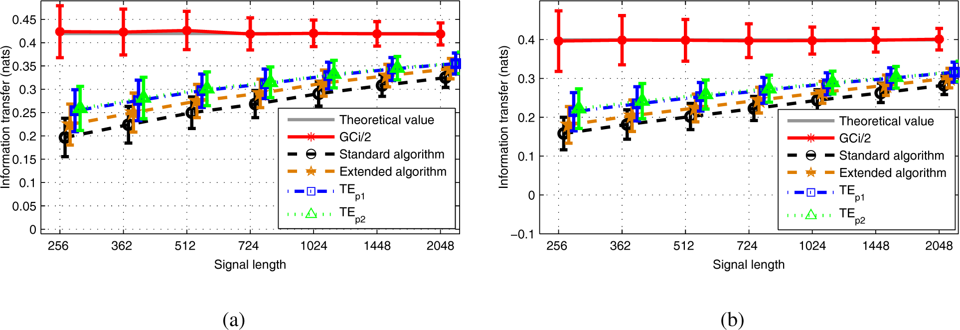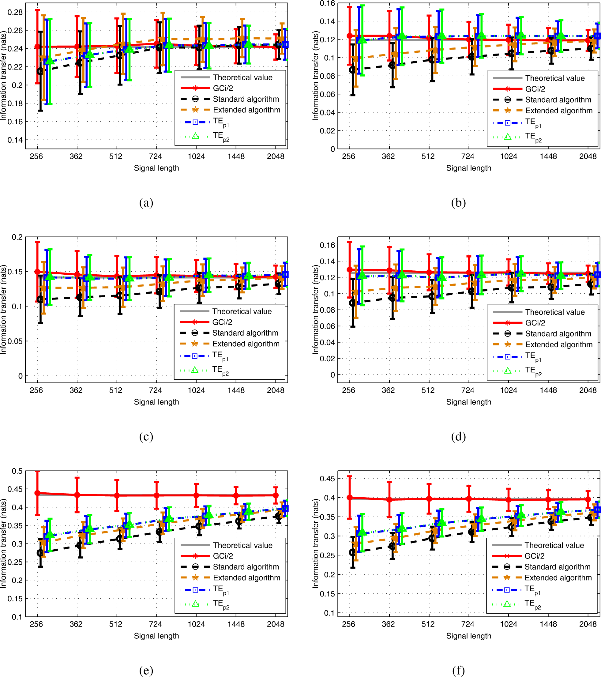Given the new entropy estimators, two novel TE estimators have been proposed, implying no extra computation cost compared to existing similar k-NN algorithm. To validate the performance of these estimators, we considered different simulated models and compared the new estimators with the two TE estimators available in the free TRENTOOL and JIDT toolboxes, respectively, and which are extensions of two Kraskov–Stögbauer–Grassberger (KSG) MI estimators, based respectively on (hyper-)cubic and (hyper-)rectangular neighborhoods.

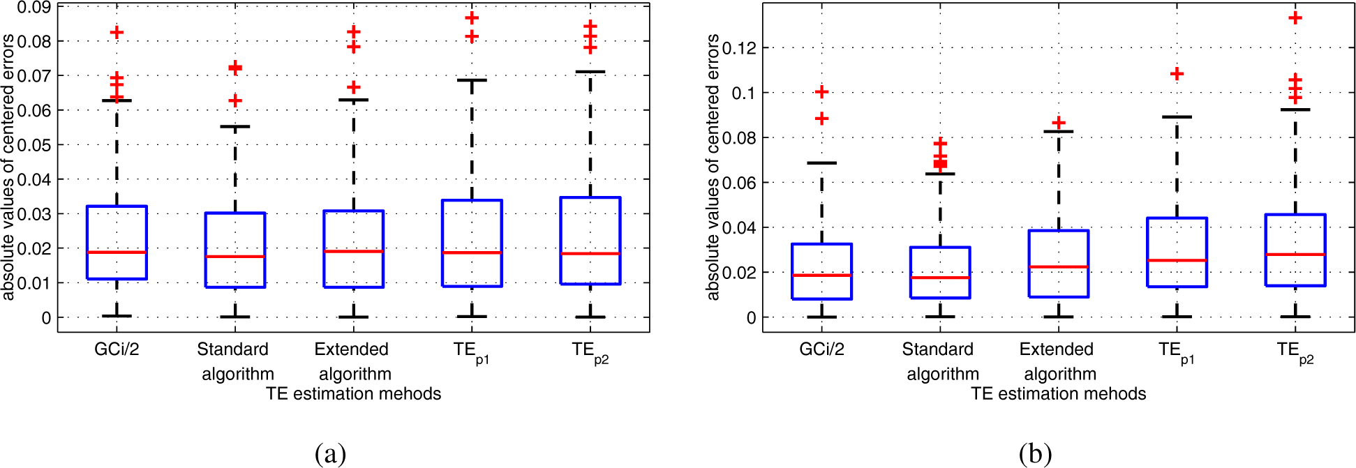
Under the Gaussian assumption, experimental results showed the effectiveness of the new estimators under the IID assumption, as well as for time-correlated AR signals in comparison with the standard KSG algorithm estimator. This conclusion still holds when comparing the new algorithms with the extended KSG estimator. Globally, all TE estimators satisfactorily converge to the theoretical TE value, i.e., to half the value of the Granger causality, while the newly proposed TE estimators showed lower bias for k sufficiently large (in comparison with the reference TE estimators) with comparable variances estimation errors.

As the variance remains relatively stable when the number of neighbors falls from eight to three, in this case, the extended algorithm, which displays a slightly lower bias, may be preferred.

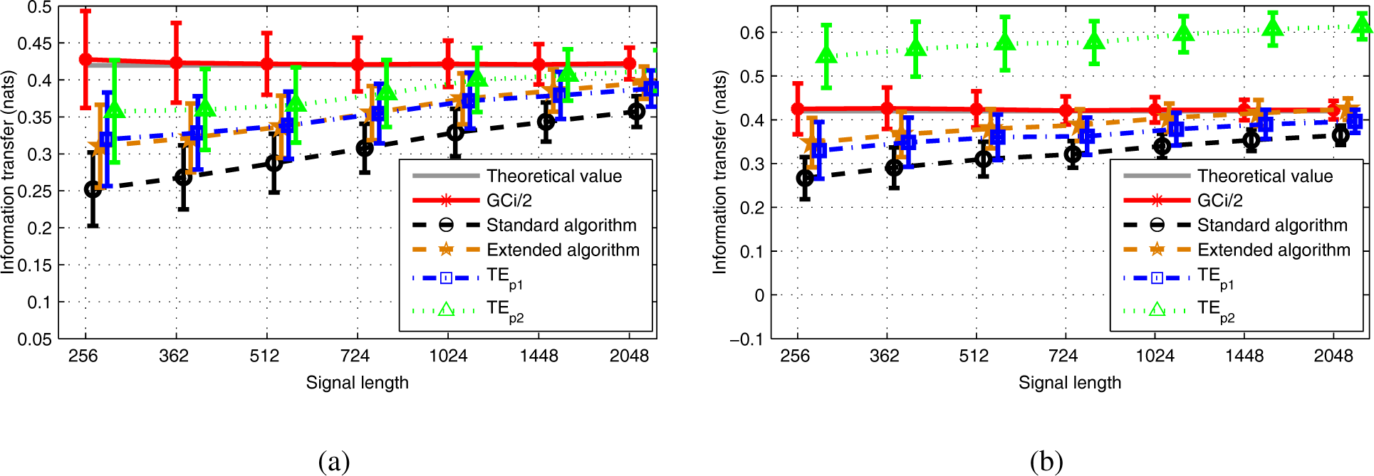
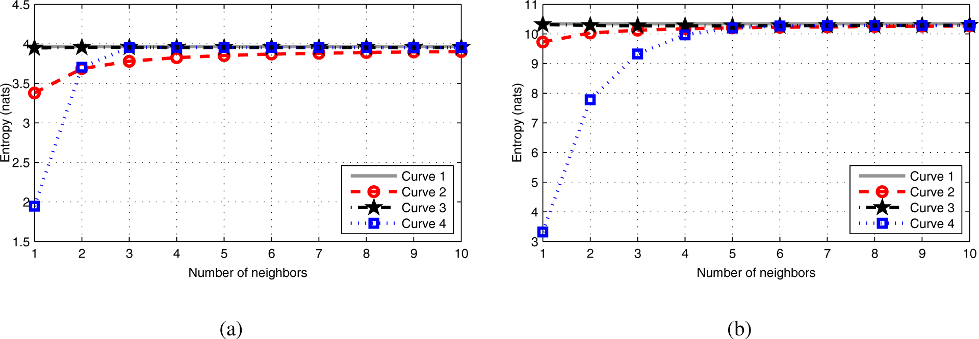
Now, one of the new TE estimators suffered from noticeable error when the number of neighbors was small. Some experiments allowed us to verify that this issue already exists when estimating the entropy of a random vector: when the number of neighbors k falls below the dimension d, then the bias drastically increases. More details on this phenomenon are given in Appendix I.

As expected, experiments with Model 1 showed that all three TE estimators under examination suffered from the “curse of dimensionality”, which made it difficult to obtain accurate estimation of TE with high dimension data. In this contribution, we do not present the preliminary results that we obtained when simulating a nonlinear version of Model 1, for which the three variables X_t, Y_t and Z_t were scalar and their joint law was non-Gaussian, because a random nonlinear transformation was used to compute X_t from Y_t, Z_t. For this model, we computed the theoretical TE (numerically, with good precision) and tuned the parameters to obtain a strong coupling between X_t and Z_t. The theoretical Granger causality index was equal to zero. We observed the same issue as that pointed out in [41], i.e., a very slow convergence of the estimator when the number of observations increases, and noticed that the four estimators $\widehat{{\mathrm{TE}}_{Y\to XSA}}$, $\widehat{{\mathrm{TE}}_{Y\to XEA}}$, $\widehat{{\mathrm{TE}}_{Y\to X_{p}1}}$ and $\widehat{{\mathrm{TE}}_{Y\to X_{p}2}}$, revealed very close performance. In this difficult case, our two methods do not outperform the existing ones. Probably, for this type of strong coupling, further improvement must be considered at the expense of an increasing computational complexity, as that proposed in [41].

This work is a first step in a more general context of connectivity investigation for neurophysiological activities obtained either from nonlinear physiological models or from clinical recordings. In this context, partial TE has also to be considered, and future work would address a comparison of the techniques presented in this contribution in terms of bias and variance. Moreover, considering the practical importance to know statistical distributions of the different TE estimators for independent channels, this point should be also addressed.