Maximum Entropy Rate Reconstruction of Markov Dynamics

Abstract

We develop ideas proposed by Van der Straeten to extend maximum entropy principles to Markov chains. We focus in particular on the convergence of such estimates in order to explain how our approach makes possible the estimation of transition probabilities when only short samples are available, which opens the way to applications to non-stationary processes. The current work complements an earlier communication by providing numerical details, as well as a full derivation of the multi-constraint two-state and three-state maximum entropy transition matrices.

1. Introduction

Probabilities play a major role in many scientific fields, from physics to social sciences. Nonetheless, assigning numerical values to the probability of some event to occur is often a difficult task, and many methods have been devised to estimate such probabilities from empirical data in an efficient way. In some cases, however, the probability space is so large, that it is not even thinkable to estimate these probabilities directly, and in such circumstances one has to resort to more or less educated guesses. The best-grounded of these assumptions relies on the maximum entropy principle [1,2], which states that, among all probability distributions satisfying some given observational constraints (for instance, given mean, correlation, marginals, etc.), the most reasonable guess is the one that has the largest Shannon entropy since entropy quantifies the amount of uncertainty in a distribution. In other words, given a constraint or a set of constraints C(p) = const, one has to maximize:

$$-{\displaystyle \sum _{x}p(x)\ln p(x)+\mathrm{\lambda }C(p(x))}$$

(1)

in order to produce a p(x) as unbiased as possible.

While originally devised in the context of statistical mechanics, the principle of maximum entropy (MaxEnt) found its way in many different research areas, from biology to linguistics, where it is now successfully employed [3–7]. More recently, several attempts to generalize this principle to dynamical situations have been proposed in different fields [8–12]. For instance, [11] studied the dynamical properties of starling flocks, while [12] tried the maximum entropy approach on financial time series, and [8] tackled the problem from the viewpoint of hidden Markov models (for completeness of the historical background, one should mention here the many pending controversies raised when extending the results of thermodynamics to non-equilibrium situations, but this topic is too far from our present concern). In all such attempts, nonetheless, one has to keep in mind that the relevance of maximum entropy methods depends tightly on the existence of sensible constraints that can be implemented easily.

In this paper, we focus on an approach presented in [13], which naturally encompasses the temporal aspect, and attempt putting appropriate emphasis on the choice of constraints. The purpose of this method is no longer to estimate a probability distribution, but to reconstruct the transition probabilities of a Markov dynamics, based on the criterion that the entropy rate of the process should be maximized. Though quite similar in spirit to the usual MaxEnt method, maximizing the entropy rate raises some extra technicalities that we discuss in the following. In a recent letter, we have shown [14] that this approach has some properties that make it suitable to inference on high-frequency datasets, in the sense that for short historical samples, the MaxEnt approach could be more efficient than usual sampling. The current paper therefore aims at recapitulating basic results derived in [13] and presents additional details, as well as new material regarding part of the work originally presented in [14].

2. Theory

Let us define a stochastic process on a discrete state space Γ by specifying its initial probability p(x) to be in state x, as well as the elements W (x, y) of its transition matrix W. This denotes the probability of switching from state x to state y in one time step.

If such a process is stationary, its entropy rate, or entropy-per-symbol, is given by [15]:

$$h=-{\displaystyle \sum _{u,\upsilon }p(u)W(u,\upsilon )\ln W(u,\upsilon )}.$$

(2)

The stationarity of the process implies that $p_t(y)=p_t{}_{+1}(y)={\displaystyle {\sum }_x{p}_t(x)W(x,y)}$, or in matrix notation p = pW. W and p are therefore not independent parameters of the process, since the latter has to be the eigenvector of the unitary eigenvalue of the former. Following [13], we will actually impose a detailed balance in order to guarantee the stationarity, that is we impose p(x)W (x, y) = p(y)W (y, x).

The detailed balance also allows us to derive a straightforward expression for the stationary probability. Indeed, using the probabilistic normalization and the detailed balance, we get:

$$p(x)=1-{\displaystyle \sum _{y\ne x}p(y)=1-{\displaystyle \sum _{y\ne x}\frac{p(x)W(x,y)}{W(y,x)}}=1-p(x){\displaystyle \sum _{y\ne x}\frac{W(x,y)}{W(y,x)}}}$$

(3)

or:

$$p(x)={\left(1+{\displaystyle \sum _{y\ne x}\frac{W(x,y)}{W(y,x)}}\right)}^{-1}.$$

(4)

It should be emphasized that the detailed balance assumption is not innocuous, but its impact depends tightly on the way processes obeying detailed balance are distributed among all Markov processes. In the case of the two-state processes considered below, it can be shown easily that any such process satisfies detailed balance, so that our procedure is perfectly valid. For larger state spaces, this property no longer holds, and it has to be checked whether or not an arbitrary process is always close to a detail-balanced one, so that the error committed by restricting to balanced processes stays small. This point should be kept in mind later on when discussing the performance of the MaxEnt approach for state spaces of higher dimensionality.

2.1. Unconstrained Case

The process has therefore three structural constraints brought in by the normalization of the stationary probability vector, the row-normalization of W and the detailed balance condition, namely:

$${\displaystyle \sum _{x}p(x)=1}$$

(5)

$${\displaystyle \sum _{y}W(x,y)=1}\mathrm{\forall }x$$

(6)

$$p(x)W(x,y)=p(y)W(y,x)\mathrm{\forall }x,y<x.$$

(7)

In the absence of additional constraints, maximizing h amounts to maximizing the function:

$$\begin{array}{c}{L}_0:=-{\displaystyle \sum _{u,\upsilon }p(u)W(u,\upsilon )\ln W(u,\upsilon )}+{\displaystyle \sum _u\mathrm{\lambda }(u)\left({\displaystyle \sum _{\upsilon }W(u,\upsilon )-1}\right)}\\ +\mathrm{\Lambda }\left({\displaystyle \sum _{u}p(u)-1}\right)+{\displaystyle \sum _{u,\upsilon <u}\mathrm{\theta }(u,\upsilon )(p(u)W(u,\upsilon )-p(\upsilon )W(\upsilon ,u))}\end{array}$$

(8)

where Λ, λ and θ are the Lagrange multipliers associated with the constraints. After straightforward calculations, we obtain the system:

$$0=\frac{\partial L_0}{\partial W(x,x)}=-p(x)\ln W(x,x)-p(x)+\mathrm{\lambda }(x)$$

(9)

$$0=\frac{\partial L_0}{\partial W(x,y<x)}=-p(x)\ln W(x,x)-p(x)+\mathrm{\lambda }(x)+\mathrm{\theta }(x,y)p(x)$$

(10)

$$0=\frac{\partial L_0}{\partial W(x,y>x)}=-p(x)\ln W(x,y)-p(x)+\mathrm{\lambda }(x)+\mathrm{\theta }(y,x)p(x)$$

(11)

$$0=\frac{\partial L_0}{\partial p(x)}=-{\displaystyle \sum _{\upsilon }W(x,\upsilon )\ln W(x,\upsilon )+\mathrm{\Lambda }}+{\displaystyle \sum _{\upsilon <x}\mathrm{\theta }(x,\upsilon )W(x,\upsilon )}-{\displaystyle \sum _{u>x}\mathrm{\theta }(u,x)W(x,u)}$$

(12)

We use the expression for λ(x) provided by Equation (9) in Equations (10) and (11); so doing, we get:

$$\ln \frac{W(x,x)}{W(x,y)}+\mathrm{\theta }(x,y)=0$$

(13)

$$\ln \frac{W(x,x)}{W(x,y)}-\mathrm{\theta }(y,x)=0$$

(14)

Swapping arguments in the last of these two equations and adding both, we get:

$$\ln \frac{W(x,x)}{W(x,y)}+\ln \frac{W(y,y)}{W(y,x)}=0\leftrightarrow \frac{W(x,x)W(y,y)}{W(x,y)W(y,x)}=1$$

(15)

In order to deal with Equation (12), we split it in terms of diagonal, upper and lower triangular elements as:

$$\begin{array}{l}0=-W(x,x)\ln W(x,x)+\mathrm{\Lambda }\\ -{\displaystyle \sum _{\upsilon <x}(\ln W(x,\upsilon )-\mathrm{\theta }(x,\upsilon ))W(x,\upsilon )}\\ -{\displaystyle \sum _{\upsilon >x}(\ln W(x,\upsilon )+\mathrm{\theta }(\upsilon ,x))W(x,\upsilon )}.\end{array}$$

(16)

The θ multipliers can be removed from this expression by using Equations (13) and (14), and we eventually get:

$$0=\mathrm{\Lambda }-\ln W(x,x),$$

(17)

so that every diagonal element of the transition matrix takes the same value. With Equation (15), it results that:

$$W(x,y)W(y,x)=e^{2\mathrm{\Lambda }}\mathrm{\forall }x,y.$$

(18)

If we assume W (x, y) = 1/N ∀x, y, then N = e^−Λ, and the normalization constraint ${\displaystyle {\sum }_{y}W(x,y)=1}$ is satisfied. Moreover, the eigenvector of W with the unitary eigenvalue is the vector with all elements equal to 1/N, so that the detailed balance is enforced. The unconstrained maximum entropy rate process is therefore given by W, such that W (x, y) = 1/N for all x, y, as expected.

2.2. Constraints

The purpose of the maximum entropy method is to rely on observables to make a least biased guess on the probability distribution, or here the transition matrix, characterizing the system. Among the many possible observable quantities, it is crucial that the ones retained are (1) easy to measure and (2) straightforward to implement as constraints. In this paper, we shall deal explicitly with constraints on the variance and the one-step autocorrelation of the process. Besides the properties above, these constraints also have the advantage that they give insights into the strengths and limitations of the method. Nevertheless, we admit that this choice is not unique.

Therefore, we constrain:

$${\displaystyle \sum _x{x}^{2}p(x)={\mathrm{\sigma }}^2}$$

(19)

and:

$${\displaystyle \sum _{x,y}xyP(x,t;y,t+1)}={\displaystyle \sum _{x,y}xyp(x)W(x,y)=A}.$$

(20)

The target function thus becomes:

$$L:=L_0+\mathrm{\alpha }\left({\displaystyle \sum _u{u}^{2}p(u)-{\mathrm{\sigma }}^2}\right)+\mathrm{\beta }\left({\displaystyle \sum _{u,\upsilon }u\upsilon p(u)W(u,\upsilon )-A}\right),$$

(21)

where α and β are the Lagrange multipliers on variance and autocorrelation, respectively. The same calculations as in the unconstrained case yield eventually:

$$-p(x)\ln W(x,x)-p(x)+\mathrm{\lambda }(x)+\mathrm{\beta }{x}^{2}p(x)=0$$

(22)

$$-p(x)\ln W(x,y)-p(x)+\mathrm{\lambda }(x)+\mathrm{\theta }(x,y)p(x)+\mathrm{\beta }xyp(x)=0$$

(23)

$$-p(x)\ln W(x,y)-p(x)+\mathrm{\lambda }(x)+\mathrm{\theta }(y,x)p(x)+\mathrm{\beta }xyp(x)=0$$

(24)

$$-{\displaystyle \sum _{\upsilon }W(x,\upsilon )\ln W(x,\upsilon )+\mathrm{\Lambda }}+{\displaystyle \sum _{\upsilon <x}\mathrm{\theta }(x,\upsilon )W(x,\upsilon )}-{\displaystyle \sum _{\upsilon >x}\mathrm{\theta }(\upsilon ,x)W(x,\upsilon )+\mathrm{\alpha }{x}^2+\mathrm{\beta }x}{\displaystyle \sum _{\upsilon }\upsilon W(x,\upsilon )=0},$$

(25)

and by the same sequence of arguments as previously, Equations (22)–(24) can be combined into:

$$\ln \frac{W(x,x)W(y,y)}{W(x,y)W(y,x)}-\mathrm{\beta }{(x-y)}^2=0,$$

(26)

while Equation (25) can be expressed as:

$$0=-\ln W(x,x)+(\mathrm{\alpha }+\mathrm{\beta })x^2\mathrm{\Lambda }\Rightarrow \ln \frac{W(x,x)}{W(y,y)}=(\mathrm{\alpha }+\mathrm{\beta })(x^2-y^2).$$

(27)

3. Solving the Equations

3.1. Two-State Case

The system of equations formed by Equations (26) and (27) has generally to be solved numerically. Before going into details of the three-state case, we address the case of two states encoded by x ∈ {−1, +1}, which can be carried out analytically. Equations (26) and (27) then become:

$$\frac{W(-,-)W(+,+)}{W(-,+)W(+,-)}=e^{4\mathrm{\beta }}$$

(28)

$$W(-,-)=W(+,+).$$

(29)

Using Equation (29) and the normalization on rows, Equation (28) can be solved easily to yield:

$$W(-,-)=\frac{1}{1+e^{-2\mathrm{\beta }}}.$$

(30)

We find therefore that the process having the highest possible entropy rate, under constrained variance and autocorrelation, is the one generated by the transition matrix:

$${\mathbf{W}}_{ME}=\left(\begin{array}{cc}\frac{1}{1+e^{-2\mathrm{\beta }}}& \frac{1}{1+e^{2\mathrm{\beta }}}\\ \frac{1}{1+e^{2\mathrm{\beta }}}& \frac{1}{1+e^{-2\mathrm{\beta }}}\end{array}\right).$$

(31)

This result can be re-expressed as a function of the observed one-step autocorrelation A. Computing the autocorrelation A′ of the MaxEnt matrix Equation (31), equating this expression to A and inverting yields $\mathrm{\beta }=\frac{1}{2}\ln \left(\frac{1+A}{1-A}\right)$. It follows that W_ME can be rewritten as:

$${\mathbf{W}}_{ME}=\left(\begin{array}{cc}\frac{1+A}{2}& \frac{1-A}{2}\\ \frac{1-A}{2}& \frac{1+A}{2}\end{array}\right).$$

(32)

Note that constraining the variance of the process has no effect, since, for the encoding of states chosen here, we get by necessity σ² = 1 for any W. It is interesting to note how the consideration of one non-trivial constraint squeezes the space on independent transition coefficients onto a one-dimensional submanifold, while enhancing multiple (consistent) constraints would result in a MaxEnt submanifold of larger dimensionality.

3.2. Three-State Case

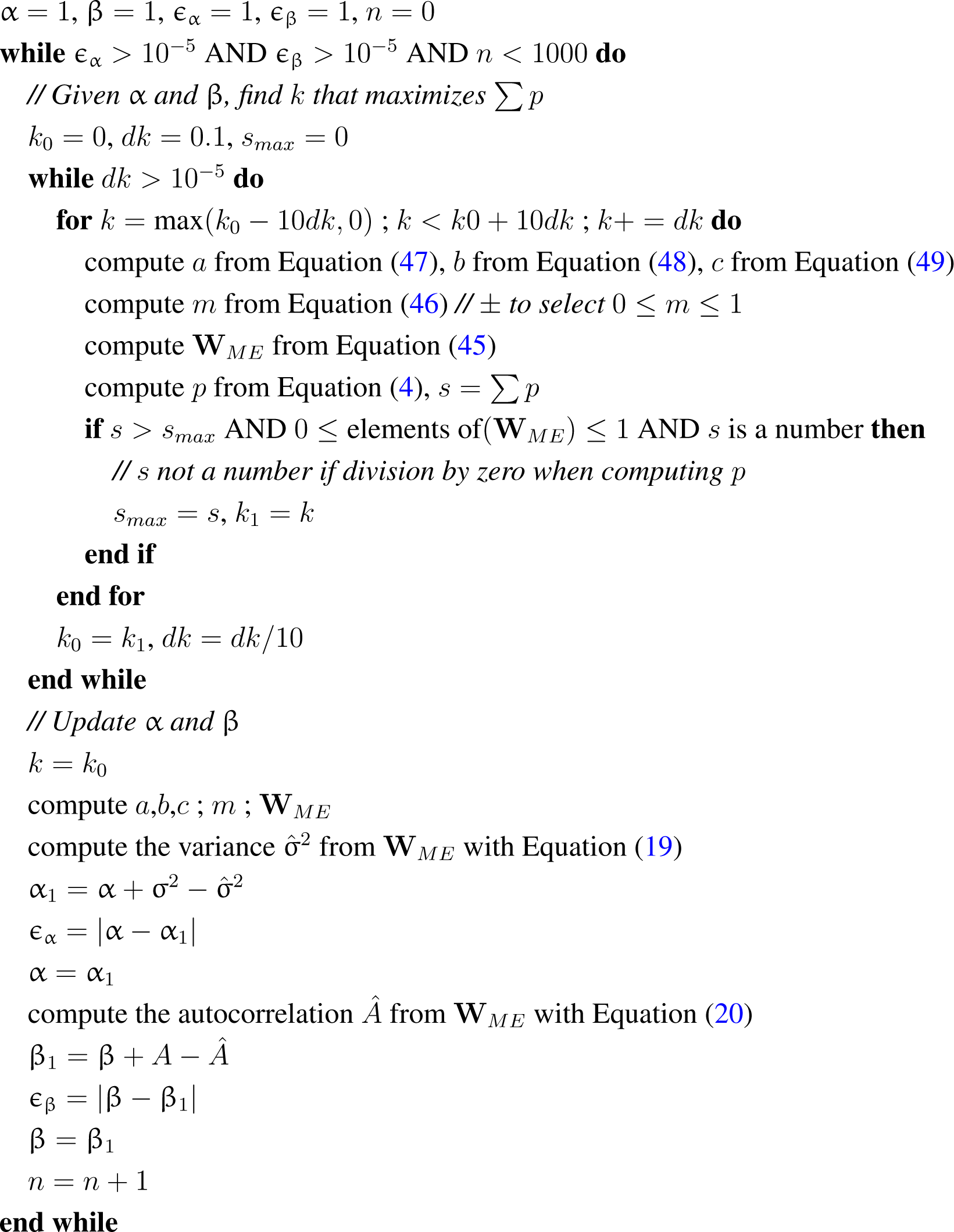
For a larger state space, the last part of the procedure has to be carried out numerically. Let us tackle the case of a three-state process, the states of which are encoded as {−1, 0, +1}. Equation (27) becomes:

$$\frac{W(-,-)}{W(0,0)}=e^{\mathrm{\alpha }+\mathrm{\beta }}$$

(33)

$$\frac{W(0,0)}{W(+,+)}=e^{-\mathrm{\alpha }-\mathrm{\beta }}$$

(34)

$$\frac{W(-,-)}{W(+,+)}=1,$$

(35)

while Equation (26) gives:

$$\frac{W(-,-)W(0,0)}{W(-,0)W(0,-)}=e^{\mathrm{\beta }}$$

(36)

$$\frac{W(-,-)W(+,+)}{W(-,+)W(+,-)}=e^{4\mathrm{\beta }}$$

(37)

$$\frac{W(0,0)W(+,+)}{W(0,+)W(+,0)}=e^{\mathrm{\beta }}.$$

(38)

The row normalization provides three equations, as well:

$$W(-,-)+W(-,0)+W(-,+)=1$$

(39)

$$W(0,-)+W(0,0)+W(0,+)=1$$

(40)

$$W(+,-)+W(+,0)+W(+,+)=1$$

(41)

Putting W (−, −) = k, we can fill up the diagonal of W_ME,

$${\mathbf{W}}_{ME}=\left(\begin{array}{ccc}k& *& *\\ *& \frac{k}{e^{\mathrm{\alpha }+\mathrm{\beta }}}& *\\ *& *& k\end{array}\right).$$

(42)

Putting W (−, 0) = m and using the condition relating W (0, −) and W (−, 0), we have:

$${\mathbf{W}}_{ME}=\left(\begin{array}{ccc}k& m& *\\ \frac{k^2}{e^{\mathrm{\alpha }+2\mathrm{\beta }}m}& \frac{k}{e^{\mathrm{\alpha }+\mathrm{\beta }}}& *\\ *& *& k\end{array}\right).$$

(43)

Then, we deal with the couple W (−, +), W (+, −), assigning W (−, +) = 1 − k − m in order to compel the normalization condition on the first row. This yields:

$${\mathbf{W}}_{ME}=\left(\begin{array}{ccc}k& m& (1-k-m)\\ \frac{k^2}{e^{\mathrm{\alpha }+2\mathrm{\beta }}m}& \frac{k}{e^{\mathrm{\alpha }+\mathrm{\beta }}}& *\\ \frac{k^2}{e^{4\mathrm{\beta }}(1-k-m)}& *& k\end{array}\right).$$

(44)

Carrying out the same procedure for the couple W (0, +), W (+, 0) and using the normalization condition on the second line gives:

$${\mathbf{W}}_{ME}=\left(\begin{array}{ccc}k& m& (1-k-m)\\ \frac{k^2}{e^{\mathrm{\alpha }+2\mathrm{\beta }}m}& \frac{k}{e^{\mathrm{\alpha }+\mathrm{\beta }}}& \left(1-\frac{k^2}{e^{\mathrm{\alpha }+2\mathrm{\beta }}m}-\frac{k}{e^{\mathrm{\alpha }+\mathrm{\beta }}}\right)\\ \frac{k^2}{e^{4\mathrm{\beta }}(1-k-m)}& \frac{k^{2}m}{e^{\mathrm{\alpha }+2\mathrm{\beta }}m-k^2-e^{\mathrm{\beta }}km}& k\end{array}\right).$$

(45)

Enforcing the normalization condition on the third line eventually gives that:

$$m=\frac{-b\pm \sqrt{b^2-4ac}}{2a}$$

(46)

with:

$$a:=(e^{5\mathrm{\beta }}-e^{4\mathrm{\beta }})k^2-(e^{6\mathrm{\beta }+\mathrm{\alpha }}+e^{5\mathrm{\beta }})k+e^{6\mathrm{\beta }+\mathrm{\alpha }}$$

(47)

$$b:=(e^{5\mathrm{\beta }}-e^{\mathrm{\beta }})k^3-(e^{6\mathrm{\beta }+\mathrm{\alpha }}+2e^{5\mathrm{\beta }}-e^{2\mathrm{\beta }+\mathrm{\alpha }})k^2+(2e^{6\mathrm{\beta }+\mathrm{\alpha }}+e^{5\mathrm{\beta }})k-e^{6\mathrm{\beta }+\mathrm{\alpha }}$$

(48)

$$c:=(e^{4\mathrm{\beta }}-1)k^4-2e^{4\mathrm{\beta }}{k}^3+e^{4\mathrm{\beta }}{k}^2.$$

(49)

3.3. Algorithm

The transition matrix W_ME (45) needs to be numerically estimated. To this end, we implemented a version of the well-known and widely used generalized iterative scaling (GIS). Specifically, the algorithm starts from an initial solution that is iteratively adjusted to fit the constraints. Setting an initial value for α = 1.0 and β = 1.0, we iterate over k to satisfy the constraint on the normalization of p. Once a solution for k is reached for a given couple (α, β), these are updated as indicated in the pseudo-code below, and the process is iterated until α and β have converged towards values satisfying the constraints on σ² and A given by Equations (19) and (20), respectively. The procedure is summarized in Algorithm 1 below. We refer to [16] for a discussion of the convergence of the GIS and an overview of other related algorithms.

Algorithm 1. Estimation of the transition matrix W_ME in the three-state case.

Algorithm 1. Estimation of the transition matrix W_ME in the three-state case.

4. MaxEnt Estimations for Time Series

Following [14], we now investigate the accuracy and limitations of the procedure we sketched in the above sections. Again, the two-state case is special, since it can receive an analytical treatment.

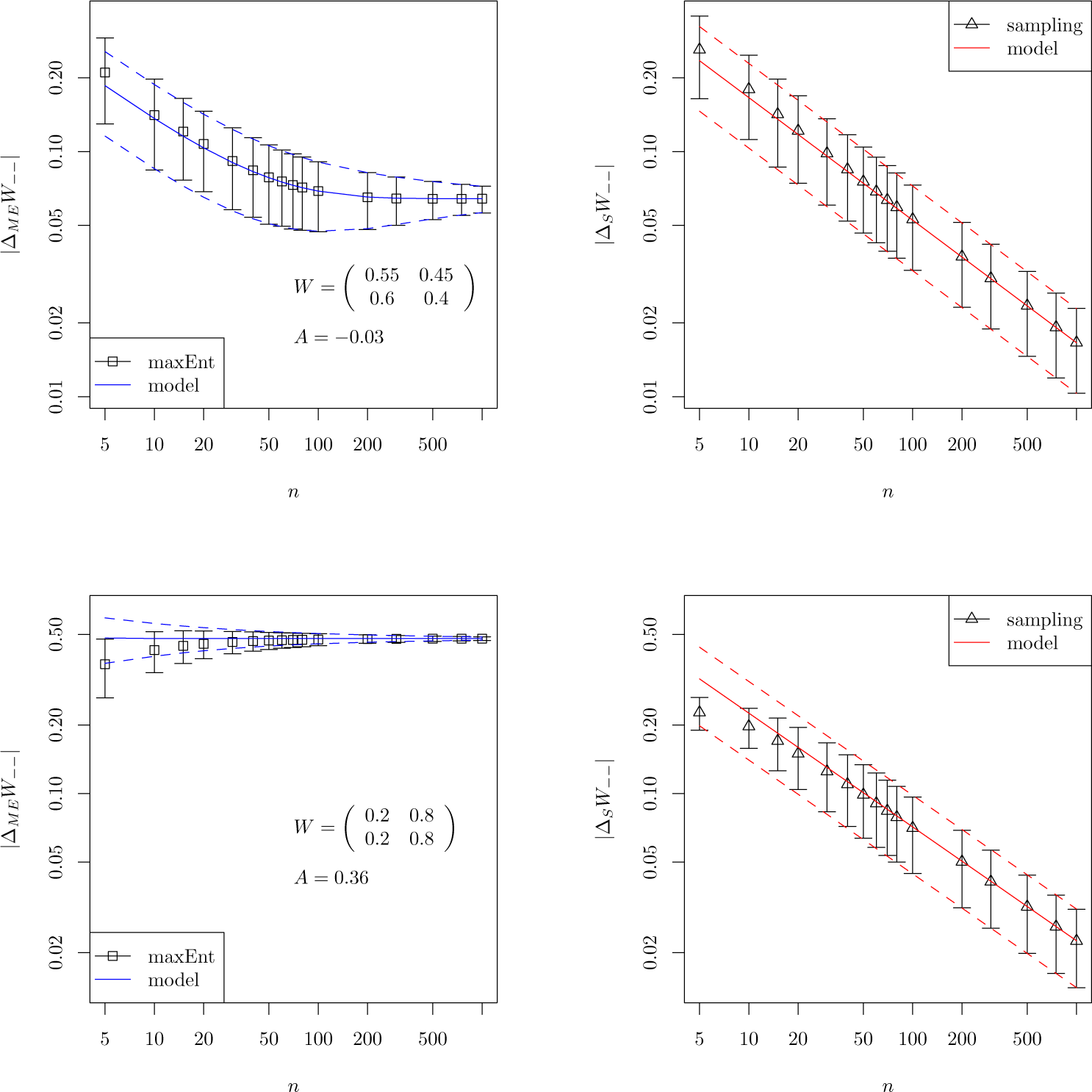
4.1. Stationary Processes

Letting A denote the autocorrelation of the process, it was shown above that in the case of a two-state process with states encoded as ±1, Equations (9) and (10) could be solved to give the MaxEnt transition matrix:

$${\mathbf{W}}_{ME}=\left(\begin{array}{cc}\frac{1+A}{2}& \frac{1-A}{2}\\ \frac{1-A}{2}& \frac{1+A}{2}\end{array}\right).$$

(50)

We now prove that there exists a subset of the space of 2 × 2 stochastic matrices for which the MaxEnt method is more efficient than sampling in estimating W when we only have short samples at our disposal. We detail the calculations for the coefficient W (−, −), the other three being similar.

Since the sample autocorrelation of a well-behaved process obeys a central limit theorem [17], we make the assumption that the sample autocorrelation A⁽ⁿ⁾ measured from a sample of size n is distributed normally according to $\mathcal{N}(A,n^{-}{}^1)$. Figure 1 shows that this estimate turns out to be quite good, even for short samples, in particular when A stays small. Here, a time series is generated from a known transition matrix and then sampled in order to reconstruct the matrix using both the MaxEnt method and histogram sampling.

According to Equation (50), it follows that the error made on the estimation of W (−, −) using the MaxEnt method is distributed as $\mathcal{N}\left(\frac{1+A}{2}-W(-,-),{(4n)}^{-1}\right)$. The absolute value of this error thus obeys a folded normal distribution, which has the mean and standard deviation given by (see [18]):

$${\langle |{\mathrm{\Delta }}_{ME}W(-,-)|\rangle }^{(n)}=\frac{e^{-2n{\mathrm{\mu }}_{--}^2}}{\sqrt{2\mathrm{\pi }n}}+{\mathrm{\mu }}_{--}(1-2\mathrm{\Phi }(-2\sqrt{n}{\mathrm{\mu }}_{--}))$$

(51)

$${\mathrm{\sigma }}^{(n)}(|{\mathrm{\Delta }}_{ME}W(-,-)|)=\sqrt{{\mathrm{\mu }}_{--}^2+\frac{1}{4n}-{\left({\langle |{\mathrm{\Delta }}_{ME}W(-,-)|\rangle }^{(n)}\right)}^2},$$

(52)

where ${\mathrm{\mu }}_{--}=\frac{1+A}{2}-W_{--}$ and Φ denotes the normal cumulative distribution.

Similarly, an estimate of the error committed when estimating W (−, −) by frequency sampling can be provided. It can be shown [19] that the coefficient sampled from a window of size n is distributed normally according to $\mathcal{N}\left(W(-,-),\frac{W(-,-)(1-W(-,-))}{n{p}_{-}}\right)$_, where p(−) denotes the stationary probability of being in state −1, which, in the current setting, is given by $p(-)=\frac{1-W(+,+)}{2-W(-,-)-W(+,+)}$. Following the same steps as previously, the sampled absolute error on W (−, −) has mean and deviation:

$${\langle |{\mathrm{\Delta }}_{S}W(-,-)|\rangle }^{(n)}=\sqrt{\frac{2W(-,-)(1-W(-,-))}{\mathrm{\pi }n{p}_{-}}}$$

(53)

$${\mathrm{\sigma }}^{(n)}(|{\mathrm{\Delta }}_{S}W(-,-)|)=\sqrt{\left(1-\frac{2}{\mathrm{\pi }}\right)\frac{W(-,-)(1-W(-,-))}{n{p}_{-}}}.$$

(54)

Equations (51) and (53) lead us to define an accuracy gain:

$${\mathrm{\Delta }}_{--}^{(n)}:={\langle |{\mathrm{\Delta }}_{S}W(-,-)|\rangle }^{(n)}-{\langle |{\mathrm{\Delta }}_{ME}W(-,-)|\rangle }^{(n)}$$

(55)

which is positive when the MaxEnt method provides a better estimation of W (−, −) than frequency sampling does for samples of size n. Though ${\mathrm{\Delta }}_{ij}^{(n)}(i,j\in \{\pm 1\})$ depends on the coefficient, one may wish to define a global Δ⁽ⁿ⁾ for the W matrix considered. While a conservative option is to choose the minimum over all coefficients, we shall rather tolerate a poor estimation of one of the coefficients as long as the corresponding transitions occur scarcely and, therefore, define ${\mathrm{\Delta }}_{\mathbf{W}}^{(n)}$ as the sum of all ${\mathrm{\Delta }}_{ij}^{(n)}’\mathrm{S}$ weighted by the stationary distribution, namely ${\mathrm{\Delta }}_{\mathbf{W}}^{(n)}={\displaystyle {\sum }_{i}p(i){\mathrm{\Delta }}_{ij}^{(n)}}$. From our experiments, the definition of ${\mathrm{\Delta }}_{\mathbf{W}}^{(n)}$ does not alter qualitatively the forthcoming results (see Figure 2). We now let n_c(W) denote the value of n above which ${\mathrm{\Delta }}_{\mathbf{W}}^{(n)}$ becomes negative. In other words, a non-negative n_c means that for historical samples shorter than n_c, the MaxEnt method gives better results when estimating the transition matrix underlying the observed process.

The quantity n_c(W) is found numerically from Equation (55) and plotted in Figure 2 over the space of 2 × 2 stochastic matrices parametrized by (W (−, −), W (+, +)). Note that n_c is large close to the diagonal, but decays when one moves away from it, which means that a matrix that is “compatible” with the structure Equation (50) is better estimated using MaxEnt.

Denoting M(n) the set of matrices, such that n_c(W) ≥ n and µ(n), the relative size of M(n) compared to M(0) (the space of all 2×2 stochastic matrices), then the relevance of the MaxEnt approach for a given state space will depend critically on the function µ(n). In the two-state case, one can read from Figure 2 that M(50) is concentrated in a neighborhood around the diagonal, so that µ(50) ≈ 0.15. This means that for samples of a size smaller than n = 50, the MaxEnt estimate is better than the frequency sampling estimate for about 15% of all possible processes. One should, however, note that processes on which one might want to apply the method are unlikely to be scattered randomly over [0, 1]², but will rather be processes having a large entropy, that is low predictability. This tends to focus our interest on the central area of [0, 1]² and increase the effective µ(n).

Though obviously µ(n) depends on the dimensionality of the state space, we were not able to set up a general argument showing how µ(n) changes when the state space gets larger. On the one hand, since an efficient frequency sampling in high-dimensional spaces should require very long samples, one might intuitively expect MaxEnt to outperform sampling in high dimensions. On the other hand, the MaxEnt procedure (in the case of one constraint put on the process) squeezes the space of independent coefficients onto a one-dimensional submanifold. The net result of these competing effects is therefore to penalize the MaxEnt approach for large state spaces. This can nevertheless be alleviated by considering extra constraints (see below), since each extra constraint increases the dimensionality of the MaxEnt submanifold.

To illustrate these points, we consider three-state processes taken randomly in regions characterized by a given range of entropy rate h. In practice, we dissected the matrix space into five regions C_i defined by the conditions h_i < h < h_max where h_max = ln 3 and h_i is specified in Figure 3; this figure shows the effectiveness of our approach by highlighting that processes having a large entropy rate are more suited to our approach. We display there the cases where two constraints are enforced (blue curves) and where the constraint on the variance of the process is relaxed (red curves). We observe that, for short samples, going from one to two constraints results in a loss of performance or at best a marginal gain, as estimation errors of constraints tend to accumulate. However, when the sampling window is long enough to allow for an accurate estimation of all constraints, adding constraints results in a spectacular improvement of the MaxEnt method.

For comparison purposes, Figure 3 also displays the success rate of the two-state processes discussed above, illustrating that MaxEnt may perform better for low-dimensional state spaces when the same number of constraints is considered.

4.2. Non-Stationary Processes

As long as only stationary processes are considered, the MaxEnt method is actually mainly of academical interest since nothing precludes the use of arbitrarily long samples. Things are very different when the dynamics itself changes over time, for then, a quick estimation of dynamical parameters becomes necessary. The crucial point, which follows immediately from our previous results, is as follows: if the coefficients W_ij(t) evolve within M(τ), where τ is the typical time scale on which the parameters of the dynamics change, then MaxEnt provides a quicker estimation of the instantaneous dynamics than sampling does.

Figure 4 conveys a qualitative illustration of this approach for a two-state stochastic process that is generated from a time-varying transition matrix:

$$\mathbf{W}(t)=\left(\begin{array}{cc}0.6+0.1\sin \left(\frac{2\mathrm{\pi }t}{T}\right)& 0.4-0.1\sin \left(\frac{2\mathrm{\pi }t}{T}\right)\\ 0.4-0.1\sin \left(\frac{2\mathrm{\pi }t}{1.2T}\right)& 0.6+0.1\sin \left(\frac{2\mathrm{\pi }t}{1.2T}\right)\end{array}\right),$$

(56)

where T = 500. Due to the relatively short period of oscillation, considering samples more than a few dozens of time units long would give meaningless over-averaged results. The figure shows that for a sliding window of size n = 50, the MaxEnt estimate (shown in blue) provides a better match of the coefficient W₋₋(t) (red). In particular, it avoids the large deviations shown by the sampling estimate (yellow).

New problems arise, however, when one attempts to deal with multiple constraints. This topic is discussed in further detail in [14], where an application is presented to quantify the risk of a financial asset.

5. Conclusions

Starting from the maximum entropy rate framework, we explained how this approach could find its utility when inferring dynamical properties of observed time series. The crucial point is that the MaxEnt approach gives more accurate estimates of the transition parameters when short samples only are available for inference. This is however true only when processes to estimate fit the structure imposed by the MaxEnt procedure, but we argue that in the case considered here, where variance and one-step autocorrelation are constrained, many processes of interest do satisfy this property. Moreover, the efficiency of the method can be drastically improved by considering multiple constraints, even though this involves extra computational issues and may, if carelessly done, significantly reduce the performance of the algorithm.

References

1. Jaynes, E.T. Information Theory Statistical Mechanics. Phys. Rev. 1957, 106, 620–630. [Google Scholar]
2. Jaynes, E.T. Information Theory Statistical Mechanics. II. Phys. Rev. 1957, 108, 171–190. [Google Scholar]
3. Schneidman, E.; Still, S.; Berry, M.J.; Bialek, W. Network Information and Connected Correlations. Phys. Rev. Lett. 2003, 91. [Google Scholar] [CrossRef]
4. Stephens, G.J.; Bialek, W. Statistical Mechanics of Letters in Words. Phys. Rev. E 2010, 81. [Google Scholar] [CrossRef]
5. Mora, T.; Bialek, W. Are Biological Systems Poised at Criticality. J. Stat. Phys. 2011, 144, 268–302. [Google Scholar]
6. Bialek, W.; Cavagna, A.; Giardina, I.; Mora, T.; Silvestri, E.; Viale, M.; Walczak, A. Statistical Mechanics for Natural Flocks of Birds. Proc. Natl. Acad. Sci. USA 2012, 109, 4786–4791. [Google Scholar]
7. Stephens, G.J.; Mora, T.; Tkacik, G.; Bialek, W. Statistical Thermodynamics of Natural Images. Phys. Rev. Lett. 2013, 110. [Google Scholar] [CrossRef]
8. McCallum, A.; Freitag, D.; Pereira, F. Maximum Entropy Markov Models for Information Extraction and Segmentation. Proceedings of the Seventeenth International Conference on Machine Learning, Standord, CA, USA, 29 June–2 July, 2000.
9. Marre, O.; El Boustani, S.; Fregnac, Y.; Destexhe, A. Prediction of Spatiotemporal Patterns of Neural Activity from Pairwise Correlations. Phys. Rev. Lett. 2009, 102, 138101. [Google Scholar]
10. Biondi, F.; Legay, A.; Nielsen, B.; Wasowski, A. Maximizing Entropy over Markov Processes. Proceedings of the 7th International Conference, Language and Automata Theory and Applications 2013, Bilbao, Spain, 2–5 April 2013; pp. 128–140.
11. Cavagna, A.; Giardina, I.; Ginelli, F.; Mora, T.; Piovani, D.; Tavarone, R.; Walczak, A. Dynamical Maximum Entropy Approach to Flocking. Phys. Rev. E 2014, 89, 042707. [Google Scholar]
12. Fiedor, P. Maximum Entropy Production Principle for Stock Returns 2014, arXiv, 1408.3728.
13. Van der Straeten, E. Maximum Entropy Estimation of Transition Probabilities of Reversible Markov Chains. Entropy. 2009, 11, 867–887. [Google Scholar]
14. Chliamovitch, G.; Dupuis, A.; Golub, A.; Chopard, B. Improving Predictability of Time Series Using Maximum Entropy Methods. Europhys. Lett. 2015, 110. [Google Scholar] [CrossRef]
15. Cover, T.; Thomas, J. Elements of Information Theory; Wiley: New York, NY, USA, 2006. [Google Scholar]
16. Malouf, R. A. Comparison of Algorithms for Maximum Entropy Parameter Estimation. Proceedings of the CoNLL-2002, Taipei, Taiwan, 31 August–1 September 2002; pp. 49–55.
17. Brockwell, P.J.; Davis, R.A. Time Series: Theory and Methods; Springer: Berlin, Germany, 1991. [Google Scholar]
18. Leone, F.C.; Nelson, L.S.; Nottingham, R.B. The Folded Normal Distribution. Technometrics 1961, 3, 867–887. [Google Scholar]
19. Brandimarte, P. Handbook in Monte Carlo Simulation: Applications in Financial Engineering, Risk Management, and Economics; Wiley: New York, NY, USA, 2014. [Google Scholar]
Figure 1. Comparison between the empirical mean and the standard deviation of data (bars) and estimate Equations (51)(54) derived from the central limit assumption (continuous lines: mean; dashed lines: standard deviation), for transition matrices with autocorrelation A = 0.03 (top) and A = 0.36 (bottom).
Entropy 17 03738f1
Figure 2. nc(W) plotted over the space of two-state stochastic matrices parametrized by W (−, −), W (+, +), for Δ W ( n ) chosen as (a) the weighted sum of individual coefficients and (b) the minimum over coefficients.
Entropy 17 03738f2
Figure 3. Success rate of three-state processes as a function of the sampling window, for two- and three-state processes involving one or two constraints. Cumulated quintiles of the entropy rate are displayed separately for three-state processes. One thousand processes are picked in each quintile.
Entropy 17 03738f3
Figure 4. A realization of the process Equation (56). The true coefficient W−−(t) (red) is compared with its MaxEnt (blue) and sampling (yellow) estimates.
Entropy 17 03738f4