Review

Log-Determinant Divergences Revisited: Alpha-Beta and Gamma Log-Det Divergences

1
Laboratory for Advanced Brain Signal Processing, Brain Science Institute, RIKEN, 2-1 Hirosawa, Wako, 351-0198 Saitama, Japan
2
Systems Research Institute, Intelligent Systems Laboratory, Newelska 6, 01-447 Warsaw, Poland
3
Dpto de Teoría de la Señal y Comunicaciones, University of Seville, Camino de los Descubrimientos s/n, 41092 Seville, Spain
4
Laboratory for Mathematical Neuroscience, RIKEN BSI, Wako, 351-0198 Saitama, Japan
*
Authors to whom correspondence should be addressed.
Entropy 2015, 17(5), 2988-3034; https://doi.org/10.3390/e17052988
Submission received: 19 December 2014 / Revised: 18 March 2015 / Accepted: 5 May 2015 / Published: 8 May 2015
(This article belongs to the Section Information Theory, Probability and Statistics)

Abstract

:
This work reviews and extends a family of log-determinant (log-det) divergences for symmetric positive definite (SPD) matrices and discusses their fundamental properties. We show how to use parameterized Alpha-Beta (AB) and Gamma log-det divergences to generate many well-known divergences; in particular, we consider the Stein’s loss, the S-divergence, also called Jensen-Bregman LogDet (JBLD) divergence, Logdet Zero (Bhattacharyya) divergence, Affine Invariant Riemannian Metric (AIRM), and other divergences. Moreover, we establish links and correspondences between log-det divergences and visualise them on an alpha-beta plane for various sets of parameters. We use this unifying framework to interpret and extend existing similarity measures for semidefinite covariance matrices in finite-dimensional Reproducing Kernel Hilbert Spaces (RKHS). This paper also shows how the Alpha-Beta family of log-det divergences relates to the divergences of multivariate and multilinear normal distributions. Closed form formulas are derived for Gamma divergences of two multivariate Gaussian densities; the special cases of the Kullback-Leibler, Bhattacharyya, Rényi, and Cauchy-Schwartz divergences are discussed. Symmetrized versions of log-det divergences are also considered and briefly reviewed. Finally, a class of divergences is extended to multiway divergences for separable covariance (or precision) matrices.

1. Introduction

Divergences or (dis)similarity measures between symmetric positive definite (SPD) matrices underpin many applications, including: Diffusion Tensor Imaging (DTI) segmentation, classification, clustering, pattern recognition, model selection, statistical inference, and data processing problems [13]. Furthermore, there is a close connection between divergence and the notions of entropy, information geometry, and statistical mean [2,47], while matrix divergences are closely related to the invariant geometrical properties of the manifold of probability distributions [4,810]. A wide class of parameterized divergences for positive measures are already well understood and a unification and generalization of their properties can be found in [1113].
The class of SPD matrices, especially covariance matrices, play a key role in many areas of statistics, signal/image processing, DTI, pattern recognition, and biological and social sciences [1416]. For example, medical data produced by diffusion tensor magnetic resonance imaging (DTI-MRI) represent the covariance in a Brownian motion model of water diffusion. The diffusion tensors can be represented as SPD matrices, which are used to track the diffusion of water molecules in the human brain, with applications such as the diagnosis of mental disorders [14]. In array processing, covariance matrices capture both the variance and correlation of multidimensional data; this data is often used to estimate (dis)similarity measures, i.e., divergences. This all has led to an increasing interest in divergences for SPD (covariance) matrices [1,5,6,14,1720].
The main aim of this paper is to review and extend log-determinant (log-det) divergences and to establish a link between log-det divergences and standard divergences, especially the Alpha, Beta, and Gamma divergences. Several forms of the log-det divergence exist in the literature, including the log–determinant α divergence, Riemannian metric, Stein’s loss, S-divergence, also called the Jensen-Bregman LogDet (JBLD) divergence, and the symmetrized Kullback-Leibler Density Metric (KLDM) or Jeffrey’s KL divergence [5,6,14,1720]. Despite their numerous applications, common theoretical properties and the relationships between these divergences have not been established. To this end, we propose and parameterize a wide class of log-det divergences that provide robust solutions and/or even improve the accuracy for a noisy data. We next review fundamental properties and provide relationships among the members of this class. The advantages of some selected log-det divergences are also discussed; in particular, we consider the efficiency, simplicity, and resilience to noise or outliers, in addition to simplicity of calculations [14]. The log-det divergences between two SPD matrices have also been shown to be robust to biases in composition, which can cause problems for other similarity measures.
The divergences discussed in this paper are flexible enough to facilitate the generation of several established divergences (for specific values of the tuning parameters). In addition, by adjusting the adaptive tuning parameters, we optimize the cost functions of learning algorithms and estimate desired model parameters in the presence of noise and outliers. In other words, the divergences discussed in this paper are robust with respect to outliers and noise if the tuning parameters, α, β, and γ, are chosen properly.

1.1. Preliminaries

We adopt the following notation: SPD matrices will be denoted by P ∈ ℝn×n and Q ∈ ℝn×n, and have positive eigenvalues λi (sorted in descending order); by log(P), det(P) = |P|, tr(P) we denote the logarithm, determinant, and trace of P, respectively.
For any real parameter α ∈ ℝ and for a positive definite matrix P, the matrix Pα is defined using symmetric eigenvalue decomposition as follows:
P α = ( V Λ V T ) α = V ( Λ α ) V T ,
where Λ is a diagonal matrix of the eigenvalues of P, and V ∈ ℝn×n is the orthogonal matrix of the corresponding eigenvectors. Similarly, we define
log P α = log ( ( V Λ V T ) α ) = V log ( Λ α ) V T ,
where log(Λ) is a diagonal matrix of logarithms of the eigenvalues of P. The basic operations for positive definite matrices are provided in Appendix A.
The dissimilarity between two SPD matrices is called a metric if the following conditions hold:
  • D(PQ) ≥ 0, where the equality holds if and only if P = Q (nonnegativity and positive definiteness).
  • D(PQ) = D(QP) (symmetry).
  • D(PZ) ≤ D(PQ) + D(QZ) (subaddivity/triangle inequality).
Dissimilarities that only satisfy condition (1) are not metrics and are referred to as (asymmetric) divergences.

2. Basic Alpha-Beta Log-Determinant Divergence

For SPD matrices P ∈ ℝn×n and Q ∈ ℝn×n, consider a new dissimilarity measure, namely, the AB log-det divergence, given by
D A B ( α , β ) ( P Q ) = 1 α β log det α ( P Q 1 ) β + β ( P Q 1 ) α α + β for α 0 , β 0 , α + β 0 ,
where the values of the parameters α and β can be chosen so as to guarantee the non-negativity of the divergence and it vanishes to zero if and only if P = Q (this issue is addressed later by Theorems 1 and 2). Observe that this is not a symmetric divergence with respect to P and Q, except when α = β. Note that using the identity log det(P) = tr log(P), the divergence in (3) can be expressed as
D A B ( α , β ) ( P Q ) = 1 α β tr [ log ( α ( P Q 1 ) β + β ( P Q 1 ) α α + β ) ] for α 0 , β 0 , α + β 0 .
This divergence is related to the Alpha, Beta, and AB divergences discussed in our previous work, especially Gamma divergences [1113,21]. Furthermore, the divergence in (4) is related to the AB divergence for SPD matrices [1,12], which is defined by
D ¯ A B ( α , β ) ( P Q ) = 1 α β tr ( α α + β P α + β + β α + β Q α + β P α Q β ) for α 0 , β 0 . α + β 0 .
Note that α and β are chosen so that D A B ( α , β ) ( P Q ) is nonnegative and equal to zero if P = Q. Moreover, such divergence functions can be evaluated without computing the inverses of the SPD matrices; instead, they can be evaluated easily by computing (positive) eigenvalues of the matrix PQ−1 or its inverse. Since both matrices P and Q (and their inverses) are SPD matrices, their eigenvalues are positive. In general, it can be shown that even though PQ−1 is nonsymmetric, its eigenvalues are the same as those of the SPD matrix Q−1/2PQ−1/2; hence, its eigenvalues are always positive.
Next, consider the eigenvalue decomposition:
( P Q 1 ) β = V Λ β V 1 ,
where V is a nonsingular matrix, and Λ β = diag { λ 1 β , λ 2 β , , λ n β } is the diagonal matrix with the positive eigenvalues λi > 0, i = 1, 2, , n, of PQ−1. Then, we can write
D A B ( α , β ) ( P Q ) = 1 α β log det α V Λ β V 1 + β V Λ α V 1 α + β = 1 α β log [ det V det α Λ β + β Λ α α + β det V 1 ] = 1 α β log det α Λ β + β Λ α α + β ,
which allows us to use simple algebraic manipulations to obtain
D A B ( α , β ) ( P Q ) = 1 α β log i = 1 n α λ i β + β λ i α α + β = 1 α β i = 1 n log ( α λ i β + β λ i α α + β ) , α , β , α + β 0 .
It is straightforward to verify that D A B ( α , β ) ( P Q ) = 0 if P = Q. We will show later that this function is nonnegative for any SPD matrices if the α and β parameters take both positive or negative values.
For the singular values α = 0 and/or β = 0 (also α = −β), the AB log-det divergence in (3) is defined as a limit for α → 0 and/or β → 0. In other words, to avoid indeterminacy or singularity for specific parameter values, the AB log-det divergence can be reformulated or extended by continuity and by applying L’Hôpital’s formula to cover the singular values of α and β. Using L’Hôpital’s rule, the AB log-det divergence can be defined explicitly by
D A B ( α , β ) ( P Q ) = { 1 α β log det α ( P Q 1 ) β + β ( Q P 1 ) α α + β for α , β 0 , α + β 0 1 α 2 [ tr ( ( Q P 1 ) α I ) α log det ( Q P 1 ) ] for α 0 , β = 0 1 β 2 [ tr ( ( P Q 1 ) β I ) β log det ( P Q 1 ) ] for α = 0 , β 0 1 α 2 log det ( P Q 1 ) α det ( I + log ( P Q 1 ) α ) for α = β 0 1 2 tr log 2 ( P Q 1 ) = 1 2 log ( Q 1 / 2 P Q 1 / 2 ) F 2 for α , β = 0 .
Equivalently, using standard matrix manipulations, the above formula can be expressed in terms of the eigenvalues of PQ−1, i.e., the generalized eigenvalues computed from λiQvi = Pvi (where vi (i = 1, 2, , n) are corresponding generalized eigenvectors) as follows:
D A B ( α , β ) ( P Q ) = { 1 α β i = 1 n log ( α λ i β + β λ i α α + β ) for α , β 0 , α + β 0 1 α 2 [ i = 1 n ( λ i α log ( λ i α ) ) n ] for α 0 , β = 0 1 β 2 [ i = 1 n ( λ i β log ( λ i β ) ) n ] for α = 0 , β 0 1 α 2 [ i = 1 n log ( λ i α 1 + log λ i α ) ] for α = β 0 1 2 i = 1 n log 2 ( λ i ) for α , β = 0 .
Theorem 1. The function D A B ( α , β ) ( P Q ) 0 given by (3) is nonnegative for any SPD matrices with arbitrary positive eigenvalues if α ≥ 0 and β ≥ 0 or if α < 0 and β < 0. It is equal to zero if and only if P = Q.
Equivalently, if the values of α and β have the same sign, the AB log-det divergence is positive independent of the distribution of the eigenvalues of PQ−1 and goes to zero if and only if all the eigenvalues are equal to one. However, if the eigenvalues are sufficiently close to one, the AB log-det divergence is also positive for different signs of α and β. The conditions for positive definiteness are given by the following theorem.
Theorem 2. The function D A B ( α , β ) ( P Q ) given by (9) is nonnegative if α > 0 and β < 0 or if α < 0 and β > 0 and if all the eigenvalues of PQ−1 satisfy the following conditions:
λ i > | β α | 1 α + β i , f o r α > 0 a n d β < 0 ,
and
λ i < | β α | 1 α + β i , f o r α < 0 a n d β > 0 .
If any of the eigenvalues violate these bounds, the value of the divergence, by definition, is infinite. Moreover, when α → −β these bounds simplify to
λ i > e 1 / α i , α = β > 0 ,
λ i < e 1 / α i , α = β < 0 .
In the limit, when α → 0 or β → 0, the bounds disappear. A visual presentation of these bounds for different values of α and β is shown in Figure 1.
Additionally, D A B ( α , β ) ( P Q ) = 0 only if λi = 1 for all i = 1, …, n, i.e., when P = Q.
The proofs of these theorems are given in Appendices B, C and D.
Figure 2 illustrates the typical shapes of the AB log-det divergence for different values of the eigenvalues for various choices of α and β.
In general, the AB log-det divergence is not a metric distance since the triangle inequality is not satisfied for all parameter values. Therefore, we can define the metric distance as the square root of the AB log-det divergence in the special case when α = β as follows:
d A B ( α , α ) ( P Q ) = D A B ( α , α ) ( P Q ) .
This follows from the fact that D A B ( α , α ) ( P Q ) is symmetric with respect to P and Q.
Later, we will show that measures defined in this manner lead to many important and well-known divergences and metric distances such as the Logdet Zero divergence, Affine Invariant Riemannian metric (AIRM), and square root of Stein’s loss [5,6]. Moreover, new divergences can be generated; specifically, generalized Stein’s loss, the Beta-log-det divergence, and extended Hilbert metrics.
From the divergence D A B ( α , α ) ( P Q ), a Riemannian metric and a pair of dually coupled affine connections are introduced in the manifold of positive definite matrices. Let dP be a small deviation of P, which belongs to the tangent space of the manifold at P. Calculating D A B ( α , β ) ( P + d P P ) and neglecting higher-order terms yields (see Appendix E)
D A B ( α , β ) ( P + d P P ) = 1 2 tr [ d P P 1 d P P 1 ] .
This gives a Riemannian metric that is common for all (α, β). Therefore, the Riemannian metric is the same for all AB log-det divergences, although the dual affine connections depend on α and β. The Riemannian metric is also the same as the Fisher information matrix of the manifold of multivariate Gaussian distributions of mean zero and covariance matrix P.
Interestingly, note that the Riemannian metric or geodesic distance is obtained from (3) for α = β = 0:
d R ( P Q ) = 2 D A B ( 0 , 0 ) ( P Q ) = tr log 2 ( P Q 1 )
= log ( P Q 1 ) F = log ( Q 1 / 2 P Q 1 / 2 ) F
= i = 1 n log 2 ( λ i ) ,
where λi are the eigenvalues of PQ−1.
This is also known as the AIRM. AIRM takes advantage of several important and useful theoretical properties and is probably one of the most widely used (dis)similarity measure for SPD (covariance) matrices [14,15].
For α = β = 0.5 (and for α = β = 0.5), the recently defined and deeply analyzed S-divergence (JBLD) [6,14,15,17] is obtained:
D S ( P Q ) = D A B ( 0.5 , 0.5 ) ( P Q ) = 4 log det ( 1 2 [ ( P Q 1 ) 1 / 2 + ( P Q 1 ) 1 / 2 ] ) = 4 log det ( P ) 1 / 2 det ( ( P Q 1 ) 1 / 2 + ( P Q 1 ) 1 / 2 2 ) det ( Q ) 1 / 2 det ( P ) 1 / 2 det ( Q ) 1 / 2 = 4 log det 1 2 ( P + Q ) det ( P ) det ( Q ) = 4 ( log det ( ( P + Q ) 2 ) 1 2 log det ( PQ ) ) = 4 i = 1 n ( λ i + 1 2 λ i ) .
The S-divergence is not a metric distance. To make it a metric, we take its square root and obtain the LogDet Zero divergence, or Bhattacharyya distance [5,7,18]:
d Bh ( P Q ) = D A B ( 0.5 , 0.5 ) ( P Q ) = 2 log det ( ( P + Q ) 2 ) 1 2 log det ( PQ ) = 2 log det 1 2 ( P + Q ) det ( P ) det ( Q ) .
Moreover, for α = 0, β ≠ 0 and α ≠ 0, β = 0, we obtain divergences which are generalizations of Stein’s loss (called also Burg matrix divergence or simply LogDet divergence):
D A B ( 0 , β ) ( P Q ) = 1 β 2 [ tr ( ( P Q 1 ) β I ) β log det ( P Q 1 ) ] , β 0 .
D A B ( α , 0 ) ( P Q ) = 1 α 2 [ tr ( ( Q P 1 ) α I ) α log det ( Q P 1 ) ] , α 0
The divergences in (22) and (23) simplify, respectively, to the standard Stein’s loss if β = 1 and to its dual loss if α = 1.

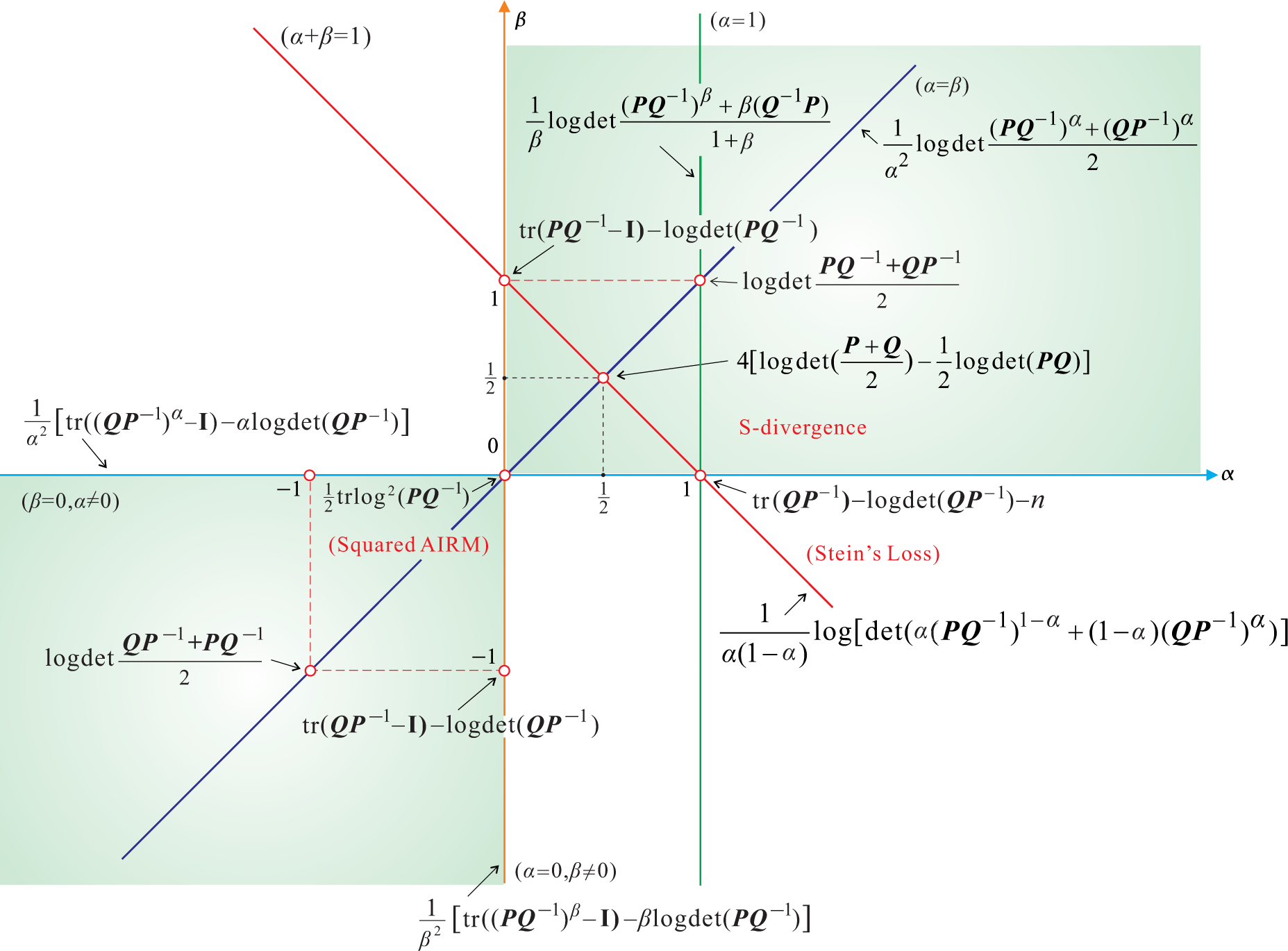
3. Special Cases of the AB Log-Det Divergence

We now illustrate how a suitable choice of the (α, β) parameters simplify the AB log-det divergence into other known divergences such as the Alpha- and Beta-log-det divergences [5,11,18,23] (see Figure 3 and Table 1).
When α + β = 1, the AB log-det divergence reduces to the Alpha-log-det divergence [5]:
D A B ( α , 1 α ) ( P Q ) = D A ( α ) ( P Q ) { 1 α ( 1 α ) log det [ α ( PQ 1 ) 1 α + ( 1 α ) ( Q P 1 ) α ] = 1 α ( 1 α ) log det ( α P + ( 1 α ) Q ) det ( P α Q 1 α ) = 1 α ( 1 α ) i = 1 n log ( α ( λ i 1 ) + 1 λ i α ) for 0 < α < 1 , tr ( Q P 1 ) log det ( Q P 1 ) n = i = 1 n ( λ i 1 + log ( λ i ) ) n for α = 1 , tr ( Q P 1 ) log det ( Q P 1 ) n = i = 1 n ( λ i log ( λ i ) ) n for α = 0 .
On the other hand, when α = 1 and β ≥ 0, the AB log-det divergence reduces to the Beta-log-det divergence:
D A B ( 1 , β ) ( P Q ) = D A ( β ) ( P Q ) { 1 β log det ( P Q 1 ) β + β ( Q P 1 ) 1 + β = 1 β i = 1 n log ( λ i β + β λ i 1 1 + β ) for β > 0 , tr ( Q P 1 I ) log det ( Q P 1 ) = i = 1 n ( λ i 1 + log ( λ i ) ) n for β = 0 , log det ( P Q 1 ) det ( I + log ( P Q 1 ) ) = i = 1 n log λ i 1 + log ( λ i ) for β = 1 , λ i > e 1 i .
Note that det ( I + log ( P Q 1 ) = Π i = 1 n [ 1 + log ( λ i ) ], and the Beta-log-det divergence is well defined for β = 1 and if all the eigenvalues are larger than λi > e−1 0.367 (e ≈ 2.72).
It is interesting to note that the Beta-log-det divergence for β → ∞ leads to a new divergence that is robust with respect to noise. This new divergence is given by
lim β D A B ( β ) ( P Q ) = D A ( ) ( P Q ) = log ( i = 1 k λ i ) for all λ i 1 .
This can be easily shown by applying the L’Hôpital’s formula. Assuming that the set Ω = {i : λi > 1} gathers the indices of those eigenvalues greater than one, we can more formally express this divergence as
D B ( ) ( P Q ) = { i Ω log λ i for Ω ϕ , 0 for Ω = ϕ .
The Alpha-log-det divergence gives the standard Stein’s losses (Burg matrix divergences) for α = 1 and α = 0, and the Beta-log-det divergence is equivalent to Stein’s loss for β = 0.
Another important class of divergences is Power log-det divergences for any α = β ∈ ℝ:
D A B ( α , α ) ( P Q ) = D P ( α ) ( P Q ) { 1 α 2 log det ( P Q 1 ) α + ( P Q 1 ) α 2 = 1 α 2 i = 1 n log λ i α + λ i α 2 for α 0 , 1 2 tr log 2 ( P Q 1 ) = 1 2 tr log 2 ( P Q 1 ) = 1 2 i = 1 n log 2 ( λ i ) for α 0 .

4. Properties of the AB Log-Det Divergence

The AB log-det divergence has several important and useful theoretical properties for SPD matrices.
  • Nonnegativity; given by
    D A B ( α , β ) ( P Q ) 0 , α , β .
  • Identity of indiscernibles (see Theorems 1 and 2); given by
    D A B ( α , β ) ( P Q ) = 0 if and only if P = Q .
  • Continuity and smoothness of D A B ( α , α ) ( P Q ) as a function of α ∈ ℝ and β ∈ ℝ, including the singular cases when α = 0 or β = 0, and when α = −β (see Figure 2).
  • The divergence can be expressed in terms of the diagonal matrix Λ = diag{λ1, λ2, , λn} with the eigenvalues of PQ−1, in the form
    D A B ( α , β ) ( P Q ) = D A B ( α , β ) ( Λ I ) .
  • Scaling invariance; given by
    D A B ( α , β ) ( c P c Q ) = D A B ( α , β ) ( P Q ) ,
    for any c > 0.
  • Relative invariance for scale transformation: For given α and β and nonzero scaling factor ω ≠ 0, we have
    D A B ( ω α , ω β ) ( P Q ) = 1 ω 2 D A B ( α , β ) ( ( Q 1 / 2 P Q 1 / 2 ) ω I ) .
  • Dual-invariance under inversion (for ω = 1); given by
    D A B ( α , β ) ( P Q ) = D A B ( α , β ) ( P 1 Q 1 ) .
  • Dual symmetry; given by
    D A B ( α , β ) ( P Q ) = D A B ( β , α ) ( Q P ) .
  • Affine invariance (invariance under congruence transformations); given by
    D A B ( α , β ) ( AP A T AQ A T ) = D A B ( α , β ) ( P Q ) ,
    for any nonsingular matrix A ∈ ℝn×n
  • Divergence lower-bound; given by
    D A B ( α , β ) ( X T PX X T QX ) D A B ( α , β ) ( P Q ) ,
    for any full-column rank matrix X ∈ ℝn×m with n ≤ m.
  • Scaling invariance under the Kronecker product; given by
    D A B ( α , β ) ( Z P Z Q ) = n D A B ( α , β ) ( P Q ) ,
    for any symmetric and positive definite matrix Z of rank n.
  • Double Sided Orthogonal Procrustes property. Consider an orthogonal matrix Ω O ( n ) and two symmetric positive definite matrices P and Q, with respective eigenvalue matrices ΛP and ΛQ which elements are sorted in descending order. The AB log-det divergence between TPΩ and Q is globally minimized when their eigenspaces are aligned, i.e.,
    min Ω O ( n ) D A B ( α , β ) ( Ω T P Ω Q ) = D A B ( α , β ) ( Λ P Λ Q ) .
  • Triangle Inequality-Metric Distance Condition, for α = β ∈ ℝ. The previous property implies the validity of the triangle inequality for arbitrary positive definite matrices, i.e.,
    D A B ( α , β ) ( P Q ) D A B ( α , α ) ( P Z ) + D A B ( α , α ) ( Z Q ) .
    The proof of this property exploits the metric characterization of the square root of the S-divergence proposed first by S. Sra in [6,17] for arbitrary SPD matrices.
Several of these properties have been already proved for the specific cases of α and β that lead to the S-divergence (α, β = 1/2) [6], the Alpha log-det divergence (0 ≤ α ≤ 1, β = 1 − α) [5] and the Riemannian metric (α, β = 0) [28, Chapter 6]. We refer the reader to Appendix F for their proofs when α, β ∈ ℝ.

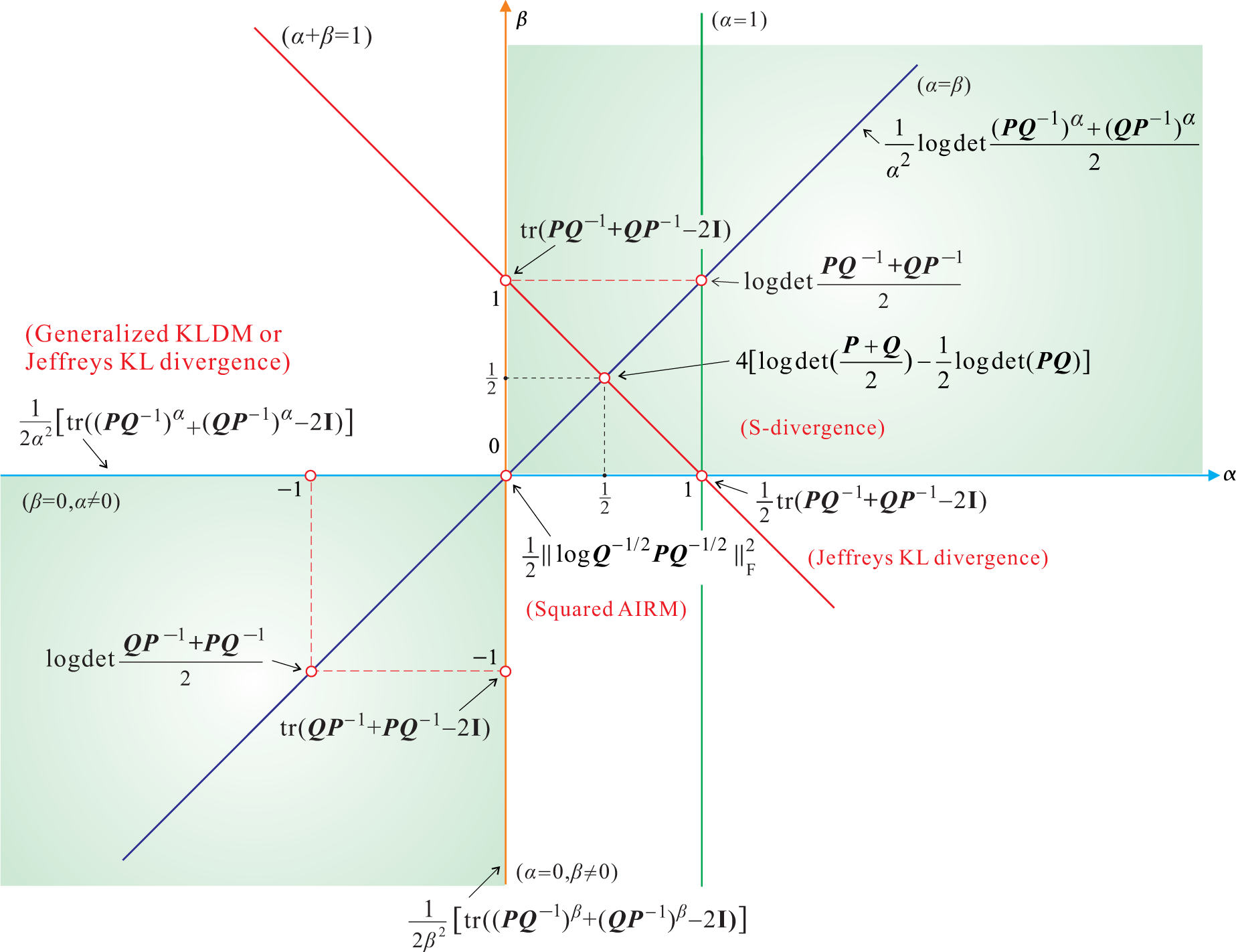
5. Symmetrized AB Log-Det Divergences

The basic AB log-det divergence is asymmetric; that is, D A B ( α , β ) ( P Q ) D A B ( α , β ) ( Q P ), except the spacial case of α = β).
In general, there are several ways to symmetrize a divergence; for example, Type-1,
D A B S 1 ( α , β ) ( P Q ) = 1 2 [ D A B ( α , β ) ( P Q ) + D A B S 1 ( α , β ) ( Q P ) ] ,
and Type-2, based on the Jensen-Shannon symmetrization (which is too complex for log-det divergences),
D A B S 2 ( α , β ) ( P Q ) = 1 2 [ D A B ( α , β ) ( P P + Q 2 ) + D A B S 1 ( α , β ) ( Q P + Q 2 ) ] .
The Type-1 symmetric AB log-det divergence is defined as
D A B S 1 ( α , β ) ( P Q ) = { 1 2 α β log det [ I + α β ( α + β ) 2 ( ( P Q 1 ) α + β + ( Q P 1 ) α + β 2 I ) ] for α β > 0 , 1 2 α 2 [ tr ( ( P Q 1 ) α + ( Q P 1 ) α 2 I ) ] for α 0 , β = 0 , 1 2 β 2 [ tr ( ( P Q 1 ) β + ( Q P 1 ) β 2 I ) ] for α = 0 , β 0 , 1 2 α 2 tr log ( I log 2 ( P Q 1 ) α ) 1 for α = β 0 , 1 2 tr log 2 ( P Q 1 ) = 1 2 log ( Q 1 / 2 P Q 1 / 2 ) F 2 for α , β = 0 .
Equivalently, this can be expressed by the eigenvalues of PQ−1 in the form
D A B S 1 ( α , β ) ( P Q ) = { 1 2 α β i = 1 n log ( 1 + α β ( α + β ) 2 ( λ i α + β 2 λ i α + β 2 ) 2 ) for α β > 0 , 1 2 α 2 i = 1 n ( λ i α + λ i α 2 ) = 1 2 α 2 i = 1 n ( λ i α 2 λ i α 2 ) 2 for α 0 , β = 0 , 1 2 β 2 i = 1 n ( λ i β + λ i β 2 ) = 1 2 β 2 i = 1 n ( λ i β 2 λ i β 2 ) 2 for α = 0 , β 0 , 1 2 α 2 i = 1 n log 1 1 log 2 ( λ i α ) for α = β 0 , 1 2 i = 1 n log 2 ( λ i ) for α , β = 0 .
We consider several well-known symmetric log-det divergences (see Figure 4); in particular, we consider the following:
  • For α = β = ±0.5, we obtain the S-divergence or JBLD divergence (20).
  • For α = β = 0, we obtain the square of the AIRM (Riemannian metric) (19).
  • For α = 0 and β = ±1 or for β = 0 and α = ±1, we obtain the KLDM (symmetrized KL Density Metric), also known as the symmetric Stein’s loss or Jeffreys KL divergence [3]:
    D J ( P Q ) = 1 2 tr ( P Q 1 + Q P 1 2 I ) = 1 2 i = 1 n ( λ i 1 λ i ) 2
One important potential application of the AB log-det divergence is to generate conditionally positive definite kernels, which are widely applied to classification and clustering. For a specific set of parameters, the AB log-det divergence gives rise to a Hilbert space embedding in the form of a Radial Basis Function (RBF) kernel [22]; more specifically, the AB log-det kernel is defined by
K A B ( α , β ) ( P Q ) = exp ( γ D A B S 1 ( α , β ) ( P Q ) ) = ( det [ I + α β ( α + β ) 2 ( ( P Q 1 ) α + β + ( Q P 1 ) α + β 2 I ) ] ) γ 2 α β
for some selected values of γ > 0 and α, β > 0 or α, β < 0 that can make the kernel positive definite.

6. Similarity Measures for Semidefinite Covariance Matrices in Reproducing Kernel Hilbert Spaces

There are many practical applications for which the underlying covariance matrices are symmetric but only positive semidefinite, i.e., their columns do not span the whole space. For instance, in classification problems, assume two classes and a set of observation vectors {x1, , xT} and {y1, , yT} in ℝm for each class, then we may wish to find a principled way to evaluate the ensemble similarity of the data from their sample similarity. The problem of the modeling of similarity between two ensembles was studied by Zhou and Chellappa in [32]. For this purpose, they proposed several probabilistic divergence measures between positive semidefinite covariance matrices in a Reproducing kernel Hilbert space (RKHS) of finite dimensionality. Their strategy was later extended for image classification problems [33] and formalized for the Log-Hilbert-Schmidt metric between infinite-dimensional RKHS covariance operators [34].
In this section, we propose the unifying framework of the AB log-det divergences to reinterpret and extend the similarity measures obtained in [32,33] for semidefinite covariance matrices in the finite-dimensional RKHS.
We shall assume that the nonlinear functions Φx : ℝmn and Φy : ℝmn (where n > m) respectively map the data from each of the classes into their higher dimensional feature spaces. We implicitly define the feature matrices as
Φ x = [ Φ x ( x 1 ) , , Φ x ( x T ) ] , Φ y = [ Φ y ( y 1 ) , , Φ y ( y T ) ] ,
and the sample covariance matrices of the observations in the feature space as: C x = Φ x J Φ x T / T n × n and C y = Φ y J Φ y T / T n × n, where J = I T 1 T 11 T denotes the T × T centering matrix.
In practice, it is common to consider low-rank approximations of sample covariance matrices. For a given basis Vx = (v1, , vr) ∈ ℝT×r of the principal subspace of J Φ x T Φ x J, we can define the projection matrix x = V x V x T and redefine the covariance matrices as
C x = 1 T Φ x V x V x T Φ x T and C y = 1 T Φ y V y V y T Φ y T .
Assuming the Gaussianity of the data in the feature space, the mean vector and covariance matrix are sufficient statistics and a natural measure of dissimilarity between Φx and Φy should be a function of the first and second order statistics of the features. Furthermore, in most practical problems the mean value should be ignored due to robustness considerations, and then the comparison reduces to the evaluation of a suitable dissimilarity measure between Cx and Cy.
The dimensionality of the feature space n is typically much larger than r, so the rank of the covariance matrices in (48) will be rn and, therefore, both matrices are positive semidefinite. The AB log-det divergence is infinite when the range spaces of the covariance matrices Cx and Cy differ. This property is useful in applications which require an automatic constraint in the range of the estimates [22], but it will prohibit the practical use of the comparison when the ranges of the covariance matrices differ. The next subsections present two different strategies to address this challenging problem.

6.1. Measuring the Dissimilarity with a Divergence Lower-Bound

One possible strategy is to use dissimilarity measures which ignore the contribution to the divergence caused by the rank deficiency of the covariance matrices. This is useful when performing one comparison of the covariances matrices after applying a congruence transformation that aligns their range spaces, and can be implemented by retaining only the finite and non-zero eigenvalues of the matrix pencil (Cx, Cy).
Let Ir denote the identity matrix of size r and (·)+ the Moore-Penrose pseudoinverse operator. Consider the eigenvalue decomposition of the symmetric matrix
( C y + ) 1 2 C x ( C y + ) 1 2 = U Λ U T
where U is a semi-orthogonal matrix for which the columns are the eigenvectors associated with the positive eigenvalues of the matrix pencil and
Λ = diag ( λ 1 , λ r ) diag E i g + { ( C y + ) 1 2 C x ( C y + ) 1 2 } .
is a diagonal matrix with the eigenvalues sorted in a descending order.
Note that the tall matrix W = ( C y + ) 1 2 U n × r diagonalizes the covariance matrices of the two classes
W T C x W = Λ
W T C y W = I r
and compress them to a common range space. The compression automatically discards the singular and infinite eigenvalues of the matrix pencil (Cx, Cy), while it retains the finite and positive eigenvalues. In this way, the following dissimilarity measures can be obtained:
L A B ( α , β ) ( C x , C y ) D A B ( α , β ) ( W T C x W W T C y W ) = D A B ( α , β ) ( Λ I r ) ,
L A B S 1 ( α , β ) ( C x , C y ) D A B S 1 ( α , β ) ( W T C x W W T C y W ) = D A B S 1 ( α , β ) ( Λ I r ) .
Note, however, that these measures should not be understood as a strict comparison of the original covariance matrices, but rather as an indirect comparison through their respective compressed versions WTCxW and WTCyW.
With the help of the kernel trick, the next lemma shows that the evaluation of the dissimilarity measures L A B ( α , β ) ( C x , C y ) and L A B S 1 ( α , β ) ( C x , C y ), does not require the explicit computation of the covariance matrices or of the feature vectors.
Lemma 1. Given the Gram matrix or kernel matrix of the input vectors
( K x x K x y K y x K y y ) = ( Φ x T Φ x Φ x T Φ y Φ y T Φ x Φ y T Φ y )
and the matrices Vx and Vy which respectively span the principal subspaces of Kxx and Kyy, the positive and finite eigenvalues of the matrix pencil can be expressed by
Λ = diag E i g + { ( V x T K x y K y y 1 V y ) ( V x T K x y K y y 1 V y ) T } .
Proof. The proof of the lemma relies on the property that for any pair of m × n matrices A and B, the non-zero eigenvalues of ABT and of BTA are the same (see [30, pag. 11]). Then, there is an equality between the following matrices of positive eigenvalues
Λ = diag E i g + { ( C y + ) 1 2 C x ( C y + ) 1 2 } = diag E i g + { C x C y + } .
Taking into account the structure of the covariance matrices in (48), such eigenvalues can be explicitly obtained in terms of the kernel matrices
E i g + { C x C y + } = E i g + { ( Φ x V x V x T Φ x T ) ( ( Φ y + ) T V y V y T Φ y T ) }
= E i g + { ( V x T Φ x T ( Φ x T ) + V y V y T Φ y + ) ( Φ x V x ) }
= E i g + { ( V x T K x y K y y 1 V y ) ( V x T K x y K y y 1 V y ) T } .

6.2. Similarity Measures Between Regularized Covariance Descriptors

Several authors consider a completely different strategy, which consists in the regularization of the original covariance matrices [3234]. This way the null the eigenvalues of the covariances Cx and Cy are replaced by a small positive constant ρ > 0, to obtain the “regularized” positive definite matrices C ˜ x and C ˜ y, respectively. The modification can be illustrated by comparing the eigendecompositions
C x = ( U x | U x ) ( Λ x 0 0 0 ) ( U x | U x ) T = U x Λ x U x T
C ˜ x = ( U x | U x ) ( Λ x 0 0 ρ I n r ) ( U x | U x ) T = C x + ρ U x ( U x ) T .
Then, the dissimilarity measure of the data in the feature space can be obtained just by measuring a divergence between the SPD matrices C ˜ x and C ˜ y. Again, the idea is to compute the value of the divergence without requiring the evaluation of the feature vectors but by using the available kernels.
Using the properties of the trace and the determinants, a practical formula for the log-det Alpha-divergence has been obtained in [32,33] for 0 < α < 1. The resulting expression
D A B ( α , 1 α ) ( C ˜ x C ˜ y ) = 1 α ( 1 α ) log det ( I 2 r + ρ 1 H ) 1 ( 1 α ) log det ( ρ 1 Λ x ) 1 α log det ( ρ 1 Λ y )
is a function of the principal eigenvalues of the kernels
Λ x = V x T K x x V x , Λ y = V x T K y y V y ,
and the matrix
H = ( ( α ) 1 2 W x 0 0 ( 1 α ) 1 2 W y ) ( K x x K x y K y x K y y ) ( ( α ) 1 2 W x 0 0 ( 1 α ) 1 2 W y ) T .
where
W x = V x ( I r ρ Λ x 1 ) 1 2 and W y = V y ( I r ρ Λ y 1 ) 1 2 .
The evaluation of the divergence outside the interval 0 < α < 1, or when β ≠ 1 − α, is not covered by this formula and, in general, requires knowledge of the eigenvalues of the matrix C ˜ y 1 2 C ˜ x C ˜ y 1 2. However, different analyses are necessary depending on the dimension of the intersection of the range space of both covariance matrices Cx and Cy. In the following, we study the two more general scenarios.
Case (A) The range spaces of Cx and Cy are the same.
In this case U y ( U y ) T = U x ( U x ) T and the eigenvalues of the matrix
C ˜ x C ˜ y 1 = ( C x + ρ U x ( U x ) T ) ( C y + + ρ 1 U x ( U x ) T )
= C x C y + + U x ( U x ) T
coincide with the nonzero eigenvalues of C x C y + except for (n − r) additional eigenvalues which are equal to 1. Then, using the equivalence between (57) and (60), the divergence reduces to the following form
D A B ( α , β ) ( C ˜ x C ˜ y ) = L A B ( α , β ) ( C x C y )
= D A B ( α , β ) ( ( V x T K x y K y y 1 V y ) ( V x T K x y K y y 1 V y ) T I r ) .
Case (B) The range spaces of Cx and Cy are disjoint.
In practice, for nr this is the most probable scenario. In such a case, the r largest eigenvalues of the matrix C ˜ x C ˜ y 1 diverge as ρ tends to zero. Hence, we can not bound above these eigenvalues and, for this reason, it makes no sense to study the case of sign(α) ≠ sign(β), so in this section we assume that sign(α) = sign(β).
Theorem 3. When range spaces of Cx and Cy are disjoint and for a sufficiently small value of ρ > 0, the AB log-det divergence is closely approximated by the formula
D A B ( α , β ) ( C ˜ x C ˜ y ) D A B ( α , β ) ( C x | y ( ρ ) ρ I r ) + D A B ( β , α ) ( C y | x ( ρ ) ρ I r ) ,
where C x | y ( ρ ) (and respectively C y | x ( ρ ) by interchanging x and y) denotes the matrix
C x | y ( ρ ) = Λ x ρ I r ρ 2 Λ y 1 W x T K x y W y Λ y 1 W y T K y x W x .
The proof of the theorem is presented in the Appendix G. The eigenvalues of the matrices C x | y ( ρ ) and C y | x ( ρ ), estimate the r largest eigenvalues of C ˜ y 1 2 C ˜ x C ˜ y 1 2 and of its inverse C ˜ x 1 2 C ˜ y C ˜ x 1 2, respectively. The relative error in the estimation of these eigenvalues is of order O(ρ), i.e., it gradually improves as ρ tend to zero. The approximation is asymptotically exact, and C x | y ( ρ ) and C x | y ( ρ ) converge respectively to the conditional covariance matrices
C x | y = lim ρ 0 C x | y ( ρ ) = V x T K x x V x ( V x T K x y V y ) ( V x T K y y V y ) 1 ( V x T K x y V y ) T ,
C y | x = lim ρ 0 C y | x ( ρ ) = V x T K y y V y ( V y T K y x V x ) ( V x T K x x V x ) 1 ( V y T K y x V x ) T ,
while ρ I converges to the zero matrix.
In the limit, the value of the divergence is not very useful because
lim ρ 0 D A B ( α , β ) ( C ˜ x C ˜ y ) =
though there are some practical ways to circumvent this limitation. For example, when α = 0 or β = 0, the divergence can be scaled by a suitable power of ρ to make it finite (see Section 3.3.1 in [32]). The scaled form of the divergence between the regularized covariance matrices is
SD A B ( α , β ) ( C ˜ x C ˜ y ) lim ρ 0 ρ max { α , β } D A B ( α , β ) ( C ˜ x C ˜ y ) .
Examples of scaled divergences are the following versions of Stein’s losses
SD A B ( 0 , β ) ( C ˜ x C ˜ y ) = lim ρ 0 ρ β D A B ( 0 , β ) ( C ˜ x C ˜ y ) = 1 β 2 tr ( ( C x | y ) β ) 0 , β > 0 ,
SD A B ( α , 0 ) ( C ˜ x C ˜ y ) = lim ρ 0 ρ α D A B ( 0 , β ) ( C ˜ x C ˜ y ) = 1 α 2 tr ( ( C y | x ) α ) 0 , α > 0 ,
as well as the Jeffrey’s KL family of symmetric divergences (cf. Equation (23) in [33])
SD A B S 1 ( α , 0 ) ( C ˜ x C ˜ y ) = lim ρ 0 ρ α D A B S 1 ( α , 0 ) ( C ˜ x C ˜ y ) = 1 2 α 2 ( tr ( ( C x | y ) α ) + tr ( ( C x | y ) α ) , α > 0 .
In other cases, when the scaling is not sufficient to obtain a finite and practical dissimilarity measure, an affine transformation may be used. The idea is to identify the divergent part of D A B ( α , β ) ( C ˜ x C ˜ y ) as ρ → 0 and use its value as a reference for the evaluation the dissimilarity. For α, β ≥ 0, the relative AB log-det dissimilarity measure is the limiting value of the affine transformation
RD A B ( α , β ) ( C ˜ x C ˜ y ) lim ρ 0 min { α , β } ( D A B S 1 ( α , 0 ) ( C ˜ x C ˜ y ) r α β log α β ρ ( α + β ) ( α + β ) 2 ) , α , β > 0 .
After its extension by continuity (including as special cases α = 0 or β = 0), the function
RD A B ( α , β ) ( C ˜ x C ˜ y ) = { log det ( C x | y ) + α β log det ( C y | x ) β > α 0 log det ( C x | y ) + log det ( C y | x ) α = β 0 log det ( C y | x ) + β α log det ( C x | y ) α > β 0
provides simple formulas to measure the relative dissimilarity between symmetric positive semidefinite matrices Cx and Cy. However, it should be taken into account that, as a consequence of its relative character, this function is not bounded below and can achieve negative values.

7. Modifications and Generalizations of AB Log-Det Divergences and Gamma Matrix Divergences

The divergence (3) discussed in the previous sections can be extended and modified in several ways. It is interesting to note that the positive eigenvalues of PQ−1 play a similar role as the ratios (pi/qi) and (qi/pi) when used in the wide class of standard discrete divergences, see for example, [11,12]; hence, we can apply such divergences to formulate a modified log-det divergence as a function of the eigenvalues λi.
For example, consider the Itakura-Saito distance defined by
D I S ( p q ) = i ( p i q i + log q i p i 1 ) .
It is worth noting that we can generate the large class of divergences or cost functions using Csiszár f-functions [13,24,25]. By replacing pi=qi with λi and qi=pi with we obtain the log-det divergence for SPD matrices:
D I S ( P Q ) = i = 1 n ( λ i log ( λ i ) ) n ,
which is consistent with (24) and (26).
As another example, consider the discrete Gamma divergence [11,12] defined by
D A C ( α , β ) ( p q ) = 1 β ( α + β ) log ( i p i α + β ) + 1 α ( α + β ) log ( i q i α + β ) 1 α β ln ( i p i α q i α ) = 1 α β ( α + β ) log ( i p i α + β ) α ( i q i α + β ) β ( i p i α q i β ) α + β , for α 0 , β 0 , α + β 0 ,
which when α = 1 and β → −1, simplifies to the following form [11]:
lim β 1 D A C ( 1 , β ) ( p q ) = 1 n i = 1 n ( log q i p i ) + log ( i = 1 n p i q i ) log ( n ) = log 1 n i = 1 n p i q i ( i = 1 n p i q i ) 1 / n .
Hence, by substituting pi/qi with λi, we derive a new Gamma matrix divergence for SPD matrices:
D C C A ( 1 , 0 ) ( P Q ) = D A C ( 1 , 1 ) ( P Q ) = 1 n i = 1 n ( log λ i 1 ) + log ( i = 1 n λ i ) log ( n ) = log 1 n i = 1 n λ i ( i = 1 n λ i ) 1 / n = log | M 1 { λ i } M 0 { λ i } ,
where M1 denotes the arithmetic mean, and M0 denotes the geometric mean.
Interestingly, (86) can be expressed equivalently as
D C C A ( 1 , 0 ) ( P Q ) = log ( tr ( P Q 1 ) ) 1 n log det ( P Q 1 ) log ( n ) .
Similarly, using the symmetric Gamma divergence defined in [11,12],
D A C S ( α , β ) ( p q ) = 1 α β log ( i p i α + β ) ( i q i α + β ) ( i p i α q i β ) ( i p i β q i α ) , for α 0 , β 0 , α + β 0 ,
for α = 1 and β → −1 and by substituting the ratios pi/qi with λi, we obtain a new Gamma matrix divergence as follows:
D A C S ( 1 , 1 ) ( P Q ) = log ( ( i = 1 n λ i ) ( i = 1 n λ i 1 ) ) log ( n ) 2 = log ( ( 1 n i = 1 n λ i ) ( 1 n i = 1 n λ i 1 ) ) = log ( M 1 { λ i } M 1 { λ i 1 } )
= log M 1 { λ i } M 1 { λ i } ,
where M1i} denotes the harmonic mean.
Note that for n → ∞, this formulated divergence can be expressed compactly as
D A C S ( 1 , 1 ) ( P Q ) = log ( E { u } E { u 1 } ) ,
where ui = {λi} and u i 1 = { λ i 1 }.
The basic means are defined as follows:
M γ ( λ ) = { M = min { λ 1 , , λ n } , γ , M 1 = n ( i = 1 n 1 λ i ) 1 , γ = 1 , M 0 = ( i = 1 n λ i ) , γ = 0 , M 1 = 1 n i = 1 n λ i , γ = 1 , M 2 = ( 1 n i = 1 n λ i 2 ) 1 / 2 , γ = 2 , M = max { λ 1 , , λ n } , γ = ,
with
M M 1 M 0 M 1 M 2 M ,
where equality holds only if all λi are equal. By increasing the values of γ, more emphasis is put on large relative errors, i.e., on λi whose values are far from one. Depending on the value of γ, we obtain the minimum entry of the vector λ (for γ → −∞), its harmonic mean (γ = 1), the geometric mean (γ = 0), the arithmetic mean (γ = 1), the quadratic mean (γ = 2), and the maximum entry of the vector (γ → ∞).
Exploiting the above inequalities for the means, the divergences in (86) and (90) can be heuristically generalized (defined) as follows:
D C C A ( γ 2 , γ 1 ) ( P Q ) = log M γ 2 { λ i } M γ 1 { λ i } ,
for γ2 > γ1.
The new divergence in (94) is quite general and flexible, and in extreme cases, it takes the following form:
D C C A ( , ) ( P Q ) = d H ( P Q ) = log M { λ i } M { λ i } = log λ m a x λ m i n ,
which is, in fact, a well-known Hilbert projective metric [6,26].
The Hilbert projective metric is extremely simple and suitable for big data because it requires only two (minimum and maximum) eigenvalue computations of the matrix PQ−1.
The Hilbert projective metric satisfies the following important properties [6,27]:
  • Nonnegativity, dH(PQ) ≥ 0, and definiteness, dH(PQ) = 0, if and only if there exists a c > 0 such that Q = cP.
  • Invariance to scaling:
    d H ( c 1 P c 2 Q ) = d H ( P Q ) ,
    for any c1, c2 > 0.
  • Symmetry:
    d H ( P Q ) = d H ( Q P ) .
  • Invariance under inversion:
    d H ( P Q ) = d H ( P 1 Q 1 ) .
  • Invariance under congruence transformations:
    d H ( AP A T AQ A T ) = d H ( P Q ) ,
    for any invertible matrix A.
  • Invariance under geodesic (Riemannian) transformations (by taking A = P−1/2 in (99)):
    d H ( I P 1 / 2 Q P 1 / 2 ) = d H ( P Q ) .
  • Separability of divergence for the Kronecker product of SPD matrices:
    d H ( P 1 P 2 Q 1 Q 2 ) = d H ( P 1 Q 1 ) + d H ( P 2 Q 2 ) .
  • Scaling of power of SPD matrices:
    d H ( P ω Q ω ) = | ω | d H ( P Q ) ,
    for any ω ≠ 0.
    Hence, for 0 < |ω1| ≤ 1 ≤ |ω2| we have
    d H ( P ω 1 Q ω 1 ) d H ( P Q ) d H ( P ω 2 Q ω 2 ) .
  • Scaling under the weighted geometric mean:
    d H ( P # s Q P # u Q ) = | s u | d H ( P Q ) ,
    for any u, s ≠ 0, where
    P # u Q = P 1 / 2 ( P 1 / 2 Q P 1 / 2 ) u P 1 / 2 .
  • Triangular inequality: d H ( P Q ) d H ( P Z ) + d H ( Z Q ).
These properties can easily be derived and verified. For example, property (9) can easily be derived as follows [6,27]:
d H ( P # s Q P # u Q ) = d H ( P 1 / 2 ( P 1 / 2 Q P 1 / 2 ) s P 1 / 2 ( P 1 / 2 ( P 1 / 2 Q P 1 / 2 ) u P 1 / 2 ) = d H ( ( P 1 / 2 Q P 1 / 2 ) s ( P 1 / 2 Q P 1 / 2 ) u ) = d H ( ( P 1 / 2 Q P 1 / 2 ) ( s u ) I ) = | s u | d H ( P Q ) .
In Table 2, we summarize and compare some fundamental properties of three important metric distances: the Hilbert projective metric, Riemannian metric, and LogDet Zero (Bhattacharyya) distance. Since some of these properties are new, we refer to [6,27,28].

7.1. The AB Log-Det Divergence for Noisy and Ill-Conditioned Covariance Matrices

In real-world signal processing and machine learning applications, the SPD sampled matrices can be strongly corrupted by noise and extremely ill conditioned. In such cases, the eigenvalues of the generalized eigenvalue (GEVD) problem Pvi = λiQvi can be divided into a signal subspace and noise subspace. The signal subspace is usually represented by the largest eigenvalues (and corresponding eigenvectors), and the noise subspace is usually represented by the smallest eigenvalues (and corresponding eigenvectors), which should be rejected; in other words, in the evaluation of log-det divergences, only the eigenvalues that represent the signal subspace should be taken into account. The simplest approach is to find the truncated dominant eigenvalues by applying the suitable threshold τ > 0; equivalently, find an index r ≤ n for which λr+1 ≤ τ and perform a summation. For example, truncation reduces the summation in (8) from 1 to r (instead of 1 to n) [22]. The threshold parameter τ can be selected via cross validation.
Recent studies suggest that the real signal subspace covariance matrices can be better represented by truncating the eigenvalues. A popular and relatively simple method applies a thresholding and shrinkage rule to the eigenvalues [35]:
λ ˜ i = λ i max { ( 1 τ γ λ γ ) , 0 } ,
where any eigenvalue smaller than the specific threshold is set to zero, and the remaining eigenvalues are shrunk. Note that the smallest eigenvalues are shrunk more than the largest one. For γ = 1, we obtain a standard soft thresholding, and for γ → ∞ a standard hard thresholding is obtained [36]. The optimal threshold τ > 0 can be estimated along with the parameter γ > 0 using cross validation. However, a more practical and efficient method is to apply the Generalized Stein Unbiased Risk Estimate (GSURE) method even if the variance of the noise is unknown (for more details, we refer to [35] and the references therein).
In this paper, we propose an alternative approach in which the bias generated by noise is reduced by suitable choices of α and β [12]. Instead of using the eigenvalues λi of PQ−1 or its inverse, we use regularized or shrinked eigenvalues [3537]. For example, in light of (8), we can use the following shrinked eigenvalues:
λ ˜ i = ( α λ i β + β λ i α α + β ) 1 α β 1 , for α , β 0 , α , β > 0 or α , β < 0 ,
which play a similar role as the ratios (pi/qi) (pi ≥ qi), which are used in the standard discrete divergences [11,12]. It should be noted that equalities λ ˜ i = 1, ∀i hold only if all λi of PQ−1 are equal to one, which occurs only if P = Q. For example, the new Gamma divergence in (94) can be formulated even more generally as
D C C A ( γ 2 , γ 1 ) ( P Q ) = log M γ 2 { λ ˜ i } M γ 1 { λ ˜ i } ,
where γ2 > γ1, and λ ˜ i are the regularized or optimally shrinked eigenvalues.

8. Divergences of Multivariate Gaussian Densities and Differential Relative Entropies of Multivariate Normal Distributions

In this section, we show the links or relationships between a family of continuous Gamma divergences and AB log-det divergences for multivariate Gaussian densities.
Consider the two multivariate Gaussian (normal) distributions:
p ( x ) = 1 ( 2 π ) n det P exp ( 1 2 ( x μ 1 ) T P 1 ( x μ 1 ) ) ,
q ( x ) = 1 ( 2 π ) n det Q exp ( 1 2 ( x μ 2 ) T Q 1 ( x μ 2 ) ) , x n ,
where µ1 ∈ ℝn and µ2 ∈ ℝn are mean vectors, and P = Σ1 ∈ ℝn×n and Q = Σ2 ∈ ℝn×n are the covariance matrices of p(x) and q(x), respectively.
Furthermore, consider the Gamma divergence for these distributions:
D A C ( α , β ) ( p ( x ) q ( x ) ) = 1 α β ( α + β ) log ( Ω p α + β ( x ) d x ) α ( Ω q α + β ( x ) d x ) β ( Ω p α ( x ) q β ( x ) d x ) α + β for α 0 , β 0 , α + β 0 ,
which generalizes a family of Gamma divergences [11,12].
Theorem 4. The Gamma divergence in (112) for multivariate Gaussian densities (110) and (111) can be expressed in closed form as follows:
D A C ( α , β ) ( p ( x ) q ( x ) ) = 1 2 D A B ( β , α ) ( ( Q 1 / 2 P Q 1 / 2 ) 1 α + β I ) + 1 2 ( μ 1 μ 2 ) T ( α Q + β P ) 1 ( μ 1 μ 2 ) , = 1 2 α β log det ( α α + β Q + β α + β P ) det ( Q ) α α + β det ( P ) β α + β + 1 2 ( α + β ) ( μ 1 μ 2 ) T ( α a + β Q + β α + β P ) 1 ( μ 1 μ 2 ) ,
for α > 0 and β > 0.
The proof is provided in Appendix H. Note that for α + β = 1, the first term in the right-hand-side of (113) also simplifies as
1 2 D A B ( β , α ) ( ( Q 1 / 2 P Q 1 / 2 ) 1 α + β I ) | β = 1 α = 1 2 D A B ( 1 α , α ) ( P Q ) = 1 2 D A ( 1 α ) ( P Q ) .
Observe that Formula (113) consists of two terms: the first term is expressed via the AB log-det divergence, which measures the similarity between two covariance or precision matrices and is independent from the mean vectors, while the second term is a quadratic form expressed by the Mahalanobis distance, which represents the distance between the means (weighted by the covariance matrices) of multivariate Gaussian distributions. Note that the second term is zero when the mean values µ1 and µ2 coincide.
Theorem 4 is a generalization of the following well-known results:
  • For α = 1 and β = 0 and as β → 0, the Kullback-Leibler divergence can be expressed as [5,38]
    lim β 0 D A C ( 1 , β ) ( p ( x ) q ( x ) ) = D K L ( p ( x ) q ( x ) ) = Ω p ( x ) log p ( x ) q ( x ) d x = 1 2 ( tr ( P Q 1 ) log det ( P Q 1 ) n ) + 1 2 ( μ 1 μ 2 ) T Q 1 ( μ 1 μ 2 ) ,
    where the last term represents the Mahalanobis distance, which becomes zero for zero-mean distributions µ1 = µ2 = 0.
  • For α = β = 0.5 we have the Bhattacharyya distance [5,39]
    D A C ( 0.5 , 0.5 ) ( p ( x ) q ( x ) ) = 1 2 d B h 2 ( p ( x ) q ( x ) ) = 4 log Ω p ( x ) q ( x ) d x = 2 log det P + Q 2 det P det Q + 1 2 ( μ 1 μ 2 ) T [ P + Q 2 ] 1 ( μ 1 μ 2 ) ,
  • For α + β = 1 and 0 < α < 1, the closed form expression for the Rényi divergence is obtained [5,32,40]:
    D A ( p q ) = 1 α ( 1 α ) log Ω p α ( x ) q 1 α ( x ) d x = 1 2 α ( 1 α ) log det ( α Q + ( 1 α ) P ) det ( Q α P 1 α ) + 1 2 ( μ 1 μ 2 ) T [ α Q + ( 1 α ) P ] 1 ( μ 1 μ 2 ) .
  • For α = β = 1, the Gamma-divergences reduce to the Cauchy-Schwartz divergence:
    D C S ( p ( x ) q ( x ) ) = log p ( x ) q ( x ) d μ ( x ) ( p 2 ( x ) d μ ( x ) ) 1 / 2 ( q 2 ( x ) d μ ( x ) ) 1 / 2 = 1 2 log det P + Q 2 det Q det P + 1 4 ( μ 1 μ 2 ) T ( P + Q 2 ) 1 ( μ 1 μ 2 ) .
Similar formulas can be derived for the symmetric Gamma divergence for two multivariate Gaussian distributions. Furthermore, analogous expressions can be derived for Elliptical Gamma distributions (EGD) [41], which facilitate more flexible modeling than standard multivariate Gaussian distributions.

8.1. Multiway Divergences for Multivariate Normal Distributions with Separable Covariance Matrices

Recently, there has been growing interest in the analysis of tensors or multiway arrays [4245]. One of the most important applications of multiway tensor analysis and multilinear distributions, is magnetic resonance imaging (MRI) (we refer to [46] and the references therein). For multiway arrays, we often use multilinear (array or tensor) normal distributions that correspond to the multivariate normal (Gaussian) distributions in (110) and (111) with common means µ1 = µ2 and separable (Kronecker structured) covariance matrices:
P ¯ = σ P 2 ( P 1 P 2 P K ) N × N
Q ¯ = σ P 2 ( Q 1 Q 2 Q K ) N × N ,
where P k = n k × n k and Q k = n k × n k for k = 1, 2, , K are SPD matrices, usually normalized so that det Pk = det Qk = 1 for each k and N = k = 1 K n k [45].
One of the main advantages of the separable Kronecker model is the significant reduction in the number of variance-covariance parameters [42]. Usually, such separable covariance matrices are sparse and very large-scale. The challenge is to design an efficient and relatively simple dissimilarity measure for big data between two zero-mean multivariate (or multilinear) normal distributions ((110) and (111)). Because of its unique properties, the Hilbert projective metric is a good candidate; in particular, for separable Kronecker structured covariances, it can be expressed very simply as
D H ( P ¯ Q ¯ ) = k = 1 K D H ( P k Q k ) = k = 1 K log λ ˜ m a x ( k ) λ ˜ m i n ( k ) = log k = 1 K ( λ ˜ m a x ( k ) λ ˜ m i n ( k ) ) ,
where λ ˜ m a x ( k ) and λ ˜ m i n ( k ) are the (shrinked) maximum and minimum eigenvalues of the (relatively small) matrices P k Q k 1 for k = 1, 2, , K, respectively. We refer to this divergence as the multiway Hilbert metric. This metric has many attractive properties, especially invariance under multilinear transformations.
Using the fundamental properties of divergence and SPD matrices, we derive other multiway log-det divergences. For example, the multiway Stein’s loss can be obtained:
D M S L ( P ¯ , Q ¯ ) = 2 D K L ( p ( x ) q ( x ) ) = D A B ( 0 , 1 ) ( P ¯ Q ¯ ) = tr ( P ¯ Q ¯ 1 ) log det ( P ¯ Q ¯ 1 ) N
= σ P 2 σ Q 2 ( k = 1 K tr ( P k Q k 1 ) ) k = 1 K N n k log det ( P k Q k 1 ) N log ( σ P 2 σ Q 2 ) N .
Note that under the constraint that det Pk = det Qk = 1, this simplifies to
D M S L ( P ¯ Q ¯ ) = tr ( P ¯ Q ¯ 1 ) log det ( P ¯ Q ¯ 1 ) N = σ P 2 σ Q 2 ( k = 1 K tr ( P k Q k 1 ) ) N log ( σ P 2 σ Q 2 ) N ,
which is different from the multiway Stein’s loss recently proposed by Gerard and Hoff [45].
Similarly, if det Pk = det Qk = 1 for each k = 1, 2, , K, we can derive the multiway Riemannian metric as follows:
D R 2 ( P ¯ Q ¯ ) = N log 2 σ P 2 σ Q 2 + k = 1 K N n k D R 2 ( P k Q k ) .
The above multiway divergences are derived using the following properties:
P ¯ Q ¯ 1 = ( P 1 P 2 P K ) ( Q 1 1 Q 2 1 Q K 1 ) = P 1 Q 1 1 P 2 Q 2 1 P K Q K 1 ,
tr ( P ¯ Q ¯ 1 ) = tr ( P 1 Q 1 1 P 2 Q 2 1 P K Q K 1 ) = k = 1 K tr ( P K Q K 1 ) ,
det ( P ¯ Q ¯ 1 ) = det ( P 1 Q 1 1 P 2 Q 2 1 P K Q K 1 ) = k = 1 K ( det ( P K Q K 1 ) ) N / n k .
and the basic property: If the eigenvalues {λi} and {θj} are eigenvalues with corresponding eigenvectors {vi} and {uj} for SPD matrices A and B, respectively, then AB has eigenvalues {λiθj} with corresponding eigenvectors {viuj}.
Other possible extensions of the AB and Gamma matrix divergences to separable multiway divergences for multilinear normal distributions under additional constraints and normalization conditions will be discussed in future works.

9. Conclusions

In this paper, we presented novel (dis)similarity measures; in particular, we considered the Alpha-Beta and Gamma log-det divergences (and/or their square-roots) that smoothly connect or unify a wide class of existing divergences for SPD matrices. We derived numerous results that uncovered or unified theoretic properties and qualitative similarities between well-known divergences and new divergences. The scope of the results presented in this paper is vast, especially since the parameterized Alpha-Beta and Gamma log-det divergence functions include several efficient and useful divergences, including those based on relative entropies, the Riemannian metric (AIRM), S-divergence, generalized Jeffreys KL (KLDM), Stein’s loss, and Hilbert projective metric. Various links and relationships between divergences were also established. Furthermore, we proposed several multiway log-det divergences for tensor (array) normal distributions.

Acknowledgments

Part of this work was supported by the Spanish Government under MICINN projects TEC2014-53103, TEC2011-23559, and by the Regional Government of Andalusia under Grant TIC-7869.

Appendices

A. Basic operations for positive definite matrices

Functions of positive definite matrices frequently appear in many research areas, for an introduction we refer the reader to Chapter 11 in [31]. Consider a positive definite matrix P of rank n with eigendecomposition VΛVT. The matrix function f(P) is defined as
f ( P ) = V f ( Λ ) V T ,
where f(Λ) diag (f1), , fn)). With the help of this definition, the following list of well-known properties can be easily obtained:
log ( det P ) = tr log ( P ) ,
( det P ) α = det ( P α ) ,
( det P ) α = det ( V Λ V T ) α = det ( V ) det ( Λ α ) det ( Λ T ) = i = 1 n λ i α ,
tr ( P α ) = tr ( V Λ V T ) α = tr ( V V T Λ α ) = i = 1 n λ i α ,
P α + β = P α P β ,
( P α ) β = P α β ,
P 0 = I ,
( det P ) α + β = det ( P α ) det ( P β ) ,
det ( ( P Q 1 ) α ) = [ det ( P ) det ( Q 1 ) ] α = det ( P α ) det ( Q α ) ,
α ( P α ) = P α log ( P ) ,
α log [ det ( P ( α ) ) ] = tr ( P 1 P α ) ,
log ( det ( P Q ) ) = n log ( det P ) + n log ( det Q ) ,
tr ( P ) log det ( P ) n .

B. Extension of D A B ( α , β ) ( P Q ) for (α, β) ∈ ℝ2

Remark 1. Equation (3) is only well defined in the first and third quadrants of the (α, β)-plane. Outside these regions, where α and β have opposite signs (i.e., α > 0 and β < 0 or α < 0 and β > 0), the divergence can be complex valued.
This undesirable behavior can be avoided with the help of the truncation operator
[ x ] + = { x x 0 , 0 , x < 0 ,
which prevents the arguments of the logarithms from being negative.
The new definition of the AB log-det divergence is
D A B ( α , β ) ( P Q ) = 1 α β log [ det α ( P Q 1 ) β + β ( P Q 1 ) α α + β ] + for α 0 , β 0 , α + β 0 ,
which is compatible with the previous definition in the first and third quadrants of the (α, β)-plane. It is also well defined in the second and fourth quadrants except for the special cases when α = 0, β = 0, and α + β = 0, which is where the formula is undefined. By enforcing continuity, we can explicitly define the AB log-det divergence on the entire (α, β)-plane as follows:
D A B ( α , β ) ( P Q ) = { 1 α β log det α ( P Q 1 ) β + β ( Q P 1 ) α α + β for α , β 0 , α + β 0 , 1 α 2 [ tr ( ( Q P 1 ) α I ) α log det ( Q P 1 ) ] for α 0 , β = 0 , 1 β 2 [ tr ( ( P Q 1 ) β I ) β log det ( P Q 1 ) ] for α = 0 , β 0 , 1 α 2 log det [ ( P Q 1 ) α ( I + log ( P Q 1 ) α ) ] + 1 for α = β , 1 2 tr log 2 ( P Q 1 ) = 1 2 log ( Q 1 / 2 P Q 1 / 2 ) F 2 for α , β = 0 .

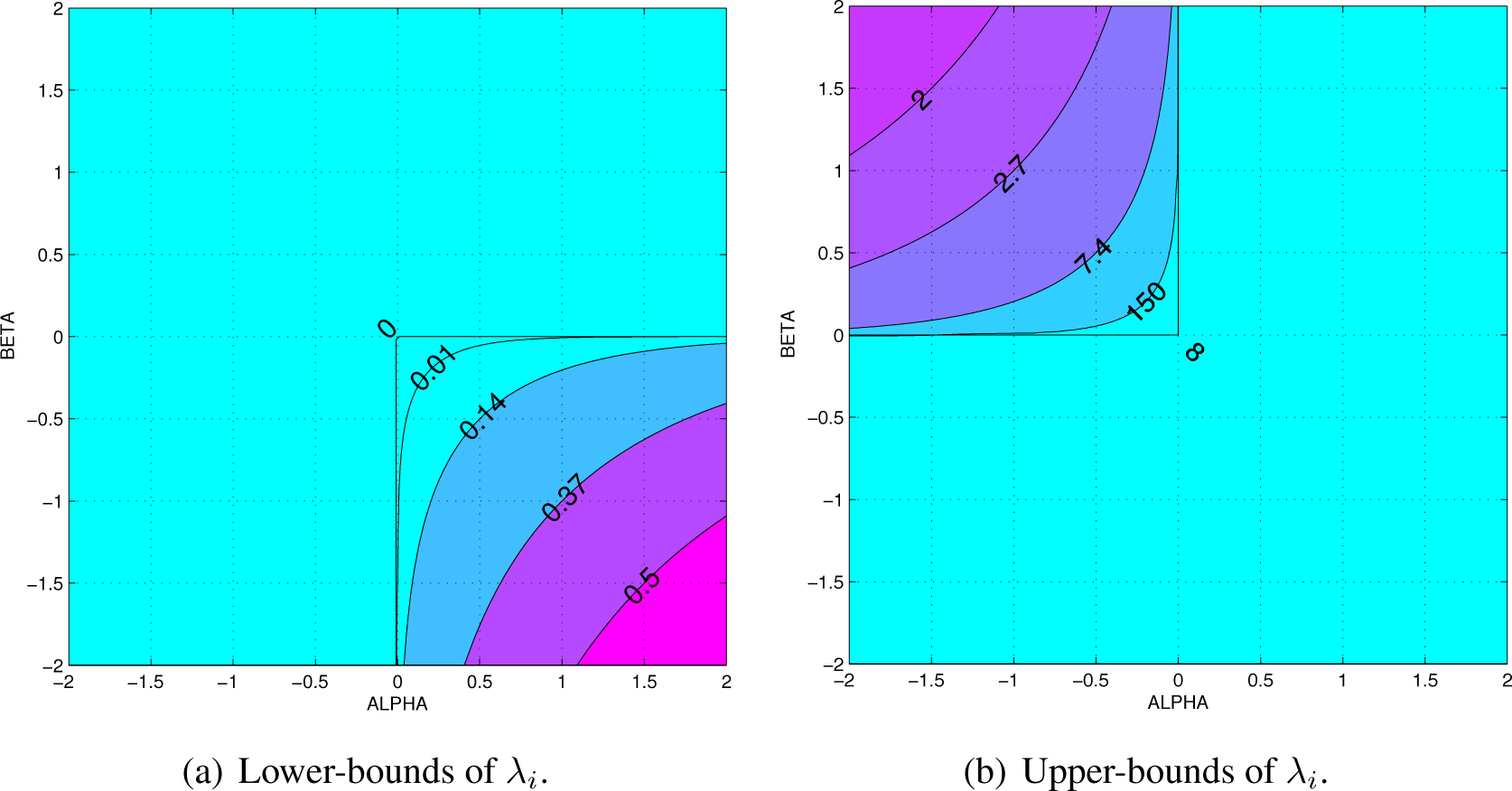
C. Eigenvalues Domain for Finite D A B ( α , β ) ( P Q )

In this section, we assume that λi, an eigenvalue of PQ−1, satisfies 0 ≤ λi ≤ ∞ for all i = 1, , n. We will determine the bounds of the eigenvalues of PQ−1 that prevent the AB log-det divergence from being infinite. First, recall that
D A B ( α , β ) ( P Q ) = 1 α β i = 1 n log [ α λ i β + β λ i α α + β ] + , α , β , α + β 0 .
We assume that 0 ≤ λi ≤ ∞ for all i. For the divergence to be finite, the arguments of the logarithms in the previous expression must be positive. This happens when
α λ i β + β λ i α α + β > 0 i ,
which is always true when α, β > 0 or when α, β < 0. On the contrary, when sign (αβ)=−1 we have the following two cases. In the first case when α > 0, we initially solve for λ i α + β and later for λi to obtain
λ i α + β α + β > β α ( α + β ) = | β α | 1 α + β λ i > | β α | 1 α + β i , for α > 0 and β < 0 .
In the second case when α < 0, we obtain
λ i α + β α + β < β α ( α + β ) = | β α | 1 α + β λ i < | β α | 1 α + β i , for α < 0 and β > 0 .
Using sign(αβ) = 1, we can solve for λ i α + β, which yields
λ i α + β α + β > | β α | 1 α + β i .
Solving again for λi, we see that
λ i > | β α | 1 α + β i , for α > 0 and β < 0 ,
and
λ i < | β α | 1 α + β i , for α < 0 and β > 0 .
In the limit, when α → −β ≠ 0, these bounds simplify to
lim α β | β α | 1 α + β = e 1 / α i , for β 0 .
On the other hand, when α → 0 or when β → 0, the bounds disappear. The lower-bounds converge to 0, while the upper-bounds converge to , leading to the trivial inequalities 0 < λi < ∞.
This concludes the determination of the domain of the eigenvalues that result in a finite divergence. Outside this domain, we expect D A B ( α , β ) ( P Q ) = . A complete picture of bounds for different values of α and β is shown in Figure 1.

D. Proof of the Nonnegativity of D A B ( α , β ) ( P Q )

The AB log-det divergence is separable; it is the sum of the individual divergences of the eigenvalues from unity, i.e.,
D A B ( α , β ) ( P Q ) = i = 1 n D A B ( α , β ) ( λ i 1 ) ,
where
D A B ( α , β ) ( λ i 1 ) = 1 α β log [ α λ i β + β λ i α α + β ] + , α , β , α + β 0 .
We prove the nonnegativity of D A B ( α , β ) ( P Q ) by showing that the divergence of each of the eigenvalues D A B ( α , β ) ( λ i 1 ) is nonnegative and minimal at λi = 1.
First, note that the only critical point of the criterion is obtained when λi = 1. This can be shown by setting the derivative of the criterion equal to zero, i.e.,
D A B ( α , β ) ( λ i 1 ) λ i = λ i α + β 1 α λ i α + β + 1 + β λ i = 0 ,
and solving for λi.
Next, we show that the sign of the derivative only changes at the critical point λi = 1. If we rewrite
D A B ( α , β ) ( λ i 1 ) λ i = ( λ i α + β 1 α + β ) ( λ i α λ i α + β + β α + β ) 1 ,
and observe that the condition for the divergence to be finite enforces α λ i α + β + β α + β > 0 then it follows that
sign { D A B ( α , β ) ( λ i 1 ) λ i } { λ i α + β 1 α + β } = { 1 for λ i < 1 , 0 , for λ i = | 1 , + 1 for λ i > 1 .
Since the derivative is strictly negative for λi < 1 and strictly positive for λi > 1, the critical point at λi = 1 is the global minimum of D A B ( α , β ) ( λ i 1 ). From this result, the nonnegativity of the divergence D A B ( α , β ) ( P Q ) 0 easily follows. Moreover, D A B ( α , β ) ( P Q ) = 0 only when λi = 1 for i = 1, …, n, which concludes the proof of the Theorems 1 and 2.

E. Derivation of the Riemannian Metric

We calculate D A B ( α , β ) ( P + d P P ) using the Taylor expansion when dP is small, i.e.,
( P + d P ) P 1 = I + d Z ,
where
d Z = d P P 1 , α [ ( P + d P ) P 1 ] β = α I + α β d Z + α β ( β 1 ) 2 d Z d Z + O ( | d Z | 3 ) .
Similar calculations hold for β[(P + dP)P−1]−α, and
α [ ( P + d P ) P 1 ] β + β [ ( P + d P ) P 1 ] α = ( α + β ) ( I + α β 2 d Z d Z ) ,
where the first-order term of dZ disappears and the higher-order terms are neglected. Since
det ( I + α β 2 d Z d Z ) = 1 + α β 2 tr ( d Z d Z ) ,
by taking its logarithm, we have
D A B ( α , β ) ( P + d P P ) = 1 2 tr ( d P P 1 d P P 1 ) ,
for any α and β.

F. Proof of the Properties of the AB Log-Det Divergence

Next we provide a proof of the properties of the AB log-det divergence. The proof will only be omitted for those properties which can be readily verified from the definition of the divergence.
  • Nonnegativity; given by
    D A B ( α , β ) ( P Q ) 0 , α , β .
    The proof of this property is presented in Appendix D.
  • Identity of indiscernibles; given by
    D A B ( α , β ) ( P Q ) = 0 if and only P = Q .
    See Appendix D for its proof.
  • Continuity and smoothness of D A B ( α , β ) ( P Q ) as a function of α ∈ ℝ and β ∈ ℝ, including the singular cases when α = 0 or β = 0, and when α = −β (see Figure 2).
  • The divergence can be explicitly expressed in terms of Λ = diag1, λ2, …, λn}, the diagonal matrix with the eigenvalues of Q−1 P; in the form
    D A B ( α , β ) ( P Q ) = D A B ( α , β ) ( Λ I ) .
    Proof. From the definition of divergence and taking into account the eigenvalue decomposition PQ−1 = VΛ V−1, we can write
    D A B ( α , β ) ( P Q ) = 1 α β log det α V Λ β V 1 + β V Λ α V 1 α + β = 1 α β log [ det V det α Λ β + β Λ α α + β det V 1 ] = 1 α β log det α Λ β + β Λ α α + β
    = D A B ( α , β ) ( Λ I ) .
  • Scaling invariance; given by
    D A B ( α , β ) ( c P c Q ) = D A B ( α , β ) ( P Q ) ,
    for any c > 0.
  • For a given α and β and nonzero scaling factor ω 6= 0, we have
    D A B ( ω , α , ω β ) ( P Q ) = 1 ω 2 D A B ( α , β ) ( ( Q 1 / 2 P Q 1 / 2 ) ω I ) .
    Proof. From the definition of divergence, we write
    D A B ( ω , α , ω β ) ( P Q ) = 1 ( ω α ) ( ω β ) log det ω α Λ ω β + ω β Λ ω α ( ω α + ω β )
    = 1 ω 2 1 α β log det α ( Λ ω ) β + β ( Λ ω ) α ( α + β )
    = 1 ω 2 D A B ( α , β ) ( ( Q 1 / 2 P Q 1 / 2 ) ω I )
    Hence, the additional inequality
    D A B ( α , β ) ( ( Q 1 / 2 P Q 1 / 2 ) ω I ) D A B ( ω , α , ω β ) ( P Q )
    is obtained for |ω| ≤ 1.
  • Dual-invariance under inversion (for ω = 1); given by
    D A B ( α , β ) ( P Q ) = D A B ( α , β ) ( P 1 Q 1 ) .
  • Dual symmetry; given by
    D A B ( α , β ) ( P Q ) = D A B ( β , α ) ( Q P ) .
  • Affine invariance (invariance under congruence transformations); given by
    D A B ( α , β ) ( AP A T AQ A T ) = D A B ( α , β ) ( P Q ) ,
    for any nonsingular matrix A n×n.
    Proof.
    D A B ( α , β ) ( AP A T AQ A T ) = 1 α β log det α ( ( AP A T AQ A T ) 1 ) β + β ( ( AP A T AQ A T ) 1 ) α α + β = 1 α β log det α ( A ( P Q 1 ) A 1 ) β + β ( A ( P Q 1 ) A 1 ) α α + β = 1 α β log [ det ( AV ) det α Λ β + β Λ α α + β det ( AV ) 1 ] = 1 α β log det α Λ β + β Λ α α + β = D A B ( α , β ) ( P Q )
  • Divergence lower-bound; given by
    D A B ( α , β ) ( X T PX X T QX ) D A B ( α , β ) ( P Q ) ,
    for any full-column rank matrix X n×m with n ≤ m.
    This result has been already proved for some special cases of α and β, especially these that lead to the S-divergence and the Riemannian metric [6]. Next, we present a different argument to prove it for any α, β ∈ ℝ.
    Proof. As already discussed, the divergence D A B ( α , β ) ( P Q ) depends on the generalized eigenvalues of the matrix pencil (P, Q), which have been denoted by λi, i = 1, …, n. Similarly, the presumed lower-bound D A B ( α , β ) ( X T PX X T QX ) is determined by µi, i = 1, …, m, the eigenvalues of the matrix pencil (XT PX, XT QX). Assuming that both sets of eigenvalues are arranged in decreasing order, the Cauchy interlacing inequalities [29] provide the following upper and lower-bounds for µj in terms of the eigenvalues of the first matrix pencil,
    λ j μ j λ n m + j .
    We classify the eigenvalues µj on three sets S μ , S μ 0 and S μ +, according to the sign of (µj 1). By the affine invariance we can write
    D A B ( α , β ) ( X T PX X T QX ) = D A B ( α , β ) ( ( X T QX ) 1 / 2 X T PX ( ( X T QX ) 1 / 2 ) I )
    = μ j S μ D A B ( α , β ) ( μ j 1 ) + μ j S μ + D A B ( α , β ) ( μ j 1 ) ,
    where the eigenvalues µj S μ 0 have been excluded since for them D A B ( α , β ) ( μ j 1 ) = 0.
    With the help of (178), the first group of eigenvalues µj S μ (which are smaller than one) are one-to-one mapped with their lower-bounds λj, which we include in the set S λ . Also those µj S μ + (which are greater than one) are mapped with their upper-bounds λnm+j, which we group in S λ +. It is shown in Appendix D that the scalar divergence D A B ( α , α ) ( λ 1 ) is strictly monotone descending for λ < 1, zero for λ = 1 and strictly monotone ascending for λ > 1. This allows one to upperbound (180) as follows
    μ j S μ D A B ( α , β ) ( μ j 1 ) + μ j S μ + D A B ( α , β ) ( μ j 1 ) μ j S λ D A B ( α , β ) ( λ j 1 ) + μ j S λ + D A B ( α , β ) ( λ j 1 ) j = 1 n D A B ( α , β ) ( λ j 1 )
    = D A B ( α , β ) ( P Q ) ,
    obtaining the desired property.
  • Scaling invariance under the Kronecker product; given by
    D A B ( α , β ) ( Z P Z Q ) = n D A B ( α , β ) ( P Q ) ,
    for any symmetric and positive definite matrix Z of rank n.
    Proof. This property was obtained in [6] for the S-divergence and the Riemannian metric. With the help of the properties of the Kronecker product of matrices, the desired equality is obtained:
    D A B ( α , β ) ( Z P Z Q ) = 1 α β log det [ α ( ( Z P ) ( Z Q ) 1 ) β + β ( ( Z Q ) ( Z P ) 1 ) α α + β ] = 1 α β log det [ α ( I P Q 1 ) β + β ( I Q P 1 ) α α + β ]
    = 1 α β log det [ I α ( P Q 1 ) β + β ( Q P 1 ) α α + β ]
    = 1 α β log det [ α ( P Q 1 ) β + β ( Q P 1 ) α α + β ] n
    = n D A B ( α , β ) ( P Q ) .
  • Double Sided Orthogonal Procrustes property. Consider an orthogonal matrix Ω O ( n ) and two symmetric positive definite matrices P and Q, with respective eigenvalue matrices ΛP and ΛQ, which elements are sorted in descending order. The AB log-det divergence between ΩT PΩ and Q is globally minimized when their eigenspaces are aligned, i.e.,
    min Ω O ( n ) D A B ( α , β ) ( Ω T P Ω Q ) = D A B ( α , β ) ( Λ P Λ Q ) .
    Proof. Let Λ denote the matrix of eigenvalues of T PΩQ−1 with its elements sorted in descending order. We start showing that for ∆ = log Λ, the function D A B ( α , β ) ( exp Δ I ) is convex. Its Hessian matrix is diagonal and positive definite, i.e., with non-negative diagonal elements
    2 D A B ( α , β ) ( e Δ i i 1 ) Δ i i 2 > 0 ,
    where
    2 D A B ( α , β ) ( e Δ i i 1 ) Δ i i 2 = { ( β α + β e α + β 2 Δ i i + α α + β e α + β 2 Δ i i ) 2 for α , α + β 0 e β Δ i i for α = 0 ( 1 + α Δ i i ) 2 for α + β = 0 e α Δ i i for β = 0
    Since f ( e Δ i i ) = D A B ( α , β ) ( e Δ i i 1 ) is strictly convex and non-negative, we are in the conditions of the Corollary 6.15 in [47]. This result states that for two symmetric positive definite matrices A and B, which vectors of eigenvalues are respectively denoted by λ A (when sorted in descending order) and λ B (when sorted in ascending order), the function f ( λ A λ B ) is submajorized by f ( λ AB ). By choosing A = T PΩ, B = Q−1, and applying the corollary, we obtain
    D A B ( α , β ) ( Λ P Λ Q ) = D A B ( α , β ) ( Λ P Λ Q 1 I ) D A B ( α , β ) ( Λ I ) = D A B ( α , β ) ( Ω P Ω Q ) ,
    where the equality is only reached when the eigendecompositions of the matrices T PΩ = P VTand Q = QVT, share the same matrix of eigenvectors V.
  • Triangle Inequality-Metric Distance Condition, for α = β ∈ ℝ; given by
    D A B ( α , α ) ( P Q ) D A B ( α , α ) ( P Z ) + D A B ( α , α ) ( Z Q ) .
    Proof. The proof of this property exploits the recent result that the square root of the S-divergence
    d Bh ( P Q ) = D S ( P Q ) = 2 log det 1 2 ( P + Q ) det ( P ) det ( Q ) .
    is a metric [17]. Given three arbitrary symmetric positive definite matrices P, Q, Z, with common dimensions, consider the following eigenvalue decompositions
    Q 1 2 P Q 1 2 = V 1 Λ 1 V 1 T
    Q 1 2 P Q 1 2 = V 2 Λ 2 V 2 T
    and assume that the diagonal matrices Λ1 and Λ2 have the eigenvalues sorted in a descending order.
    For a given value of α in the divergence, we define ω = 2α ≠ 0 and use properties 6 and 9 (see Equations (168) and (175)) to obtain the equivalence
    D A B ( α , α ) ( P Q ) = D A B ( ω 0.5 , ω 0.5 ) ( P Q ) = 1 ω 2 D A B ( 0.5 , 0.5 ) ( ( Q 1 / 2 P Q 1 / 2 ) ω I ) = 1 2 | α | D A B ( 0.5 , 0.5 ) ( Λ 1 2 α I ) = 1 2 | α | d Bh ( Λ 1 2 α I ) ,
    Since the S-divergence satisfies the triangle inequality for diagonal matrices [5,6,17]
    d Bh ( Λ 1 2 α I ) d Bh ( Λ 1 2 α Λ 2 2 α ) + d Bh ( Λ 2 2 α I ) ,
    from (196), this implies that
    D A B ( α , α ) ( P Q ) D A B ( α , α ) ( Λ 1 Λ 2 ) + D A B ( α , α ) ( Λ 2 I )
    In similarity with the proof of the metric condition for S-divergence [6], we can use property 12 to bound above the first term in the right-hand-side of the equation by
    D A B ( α , α ) ( Λ 1 Λ 2 ) D A B ( α , α ) ( Λ 1 Λ 1 Λ 1 T Λ 2 Λ 2 Λ 2 T ) = D A B ( α , α ) ( Q 1 2 P Q 1 2 Q 1 2 Z Q 1 2 ) = D A B ( α , α ) ( P Z ) ,
    whereas the second term satisfies
    D A B ( α , α ) ( Λ 2 I ) = D A B ( α , α ) ( Λ 2 Λ 2 Λ 2 T I ) = D A B ( α , α ) ( Q 1 2 P Q 1 2 I ) = D A B ( α , α ) ( Z Q ) .
    After bounding the right-hand-side of (198) with the help of (199) and (200), the divergence satisfies the desired triangle inequality (192) for α ≠ 0.
    On the other hand, D A B ( α , α ) ( P Q ) as α → 0 converges to the Riemannian metric
    D A B ( 0 , 0 ) ( P Q ) = lim α 0 D A B ( α , α ) ( P Q )
    = log ( Q 1 / 2 P Q 1 / 2 ) F
    = d R ( P Q ) .
    which concludes the proof of the metric condition of D A B ( α , α ) ( P Q ) for any α ∈ ℝ

G. Proof of Theorem 3

This theorem assumes that the range spaces of the symmetric positive semidefinite matrices Cx and Cy are disjoint, in the sense that they only intersect at the origin, which is the most probable situation for nr (where n is the size of the matrices while r is their common rank). For ρ > 0 the regularized versions C ˜ x and C ˜ y of these matrices are full rank.
Let Λ ˜ = diag ( λ ˜ 1 , , λ ˜ n ) denote the diagonal matrix representing the n eigenvalues of the matrix pencil ( C ˜ x , C ˜ y ). The AB log-det divergence between the regularized matrices is equal to the divergence between Λ ˜ and the identity matrix of size n, i.e.,
D A B ( α , β ) ( C ˜ x C ˜ y ) = D A B ( α , β ) ( C ˜ y 1 2 C ˜ x C ˜ y 1 2 I n ) = D A B ( α , β ) ( Λ ˜ I n ) .
The positive eigenvalues of the matrix pencil satisfy
Λ ˜ diag E i g + { ( C ˜ y ) 1 2 C ˜ x ( C ˜ y ) 1 2 ) } = diag E i g + { C ˜ x C ˜ y 1 2 } ,
therefore, the divergence can be directly estimated from the eigenvalues of C ˜ x C ˜ y 1. In order to simplify this matrix product, we first express C ˜ x and C ˜ y 1 in term of the auxiliary matrices
T x = U x ( Λ x ρ I r ) 1 2 and T y = U y ( Λ y ρ I r ) 1 2 .
In this way, they are written as a scaled version of the identity matrix plus a symmetric term:
C ˜ x = C x + ρ U x ( U x ) T = U x Λ x U x T + ρ ( I n U x U x T ) = ρ I n + U x ( Λ x ρ I r ) U x T = ρ I n + T x T x T ,
and
C ˜ y 1 = C y + + ρ 1 U y ( U y ) T = U y Λ y 1 U y T + ρ 1 ( I n U y U y T ) = ρ 1 I n ρ 1 U y ( Λ y + ρ I r ) Λ y 1 U y = ρ 1 I n ρ 1 T y Λ y 1 T y T .
Next, using (207) and (208), we expand the product
C ˜ x C ˜ y 1 = I n + ρ 1 T x T x T ( I n T y Λ y 1 T y T ) + R
and approximate the eigenvectors Uy Ux of the residual matrix R to obtain the estimate
R U y ( I r + ρ Λ y 1 ) U y T U x ( I r + ρ Λ y 1 ) U x T R ^ .
Hence, it is not difficult to see that the estimated residual is equal to
R ^ = T x ( I r + ρ Λ y 1 ) T x + .
After substituting (211) in (209) and collecting common terms, we obtain the expansion
C ˜ x C ˜ y 1 = I n + T x ( ρ 1 T x T ρ 1 T x T T y Λ y 1 T y T ( I r + ρ Λ y 1 ) T x + ) C ˜ x C ˜ y 1 ^ + O ( ρ 0 ) .
Let Eig1{·} denote the arrangement of the ordered eigenvalues of the matrix argument after excluding those that are equal to 1. For convenience, we reformulate the property proved in [30] that for any pair of matrices A, B ∈ ℝm×n, the non-zero eigenvalues of ABT and of BTA are the same, into the following proposition.
Proposition 1. For any pair of m × n matrices A and B, the eigenvalues of the matrices Im + ABT and In + BTA, which are not equal to 1, coincide.
E i g 1 { I m + A B T } = E i g 1 { I m + B T A }
Since range spaces of Cx and of Cy only intersect at the origin, the approximation matrix C ˜ x C ˜ y 1 ^ has r dominant eigenvalues of order O(ρ−1) and (n − r) remaining eigenvalues equal to 1. Using Proposition 1, these r dominant eigenvalues are given by
E i g 1 { C ˜ x C ˜ y 1 ^ } = E i g 1 { I r + ( ρ 1 T x T ρ 1 T x T T y Λ y 1 T y T ( I r + ρ Λ y 1 ) T x + ) T x } = E i g 1 { ρ 1 T x T T x ρ 1 T x T T y Λ y 1 T y T T x ρ Λ y 1 } .
Let Λ ˜ m a x and Λ ˜ m i n, respectively denote the diagonal submatrices of Λ ˜ with the r largest and with the r smallest eigenvalues. From the definitions in (66) and (206), one can recognize that T x T T x = Λ x ρ I r, while T x T T y = W x T K xy W y, and substituting them in (214) we obtain the estimate of the r largest eigenvalues
Λ ^ max = diag E i g 1 { C ˜ x C ˜ y 1 ^ }
= diag E i g 1 { ρ 1 Λ x I ρ Λ y 1 ρ 1 W x T K xy W y Λ y 1 W y T K yx W x } ρ 1 C x / y ( ρ ) .
The relative error between these eigenvalues and the r largest eigenvalues of C ˜ x C ˜ y 1 is of order O(ρ). This is a consequence of the fact that these eigenvalues are O(ρ−1), while the Frobenius norm of the error matrix is O(ρ0). Then, the relative error between the dominant eigenvalues of the two matrices can be bounded above by
( i = 1 r ( λ ˜ i λ ^ i ) 2 i = 1 r λ ˜ i 2 ) 1 2 C ˜ x C ˜ y 1 C ˜ x C ˜ y 1 ^ F ( i = 1 r λ ^ i 2 ) 1 2 + O ( ρ 0 ) O ( ρ 0 ) O ( ρ 1 ) O ( ρ ) .
On the other hand, the r smallest eigenvalues of Λ ^ are the reciprocal of the r dominant eigenvalues of the inverse matrix ( C ˜ y 1 2 C ˜ x C ˜ y 1 2 ) 1, so we can estimate them using essentially the same procedure
Λ ^ min 1 = diag E i g 1 { C ˜ x C ˜ y 1 ^ }
= diag E i g 1 { ρ 1 C y / x ( ρ ) } .
For a sufficient small value of ρ > 0, the dominant contribution to the AB log-det divergence comes from the r largest and r smallest eigenvalues of the matrix pencil (Ĉx, Ĉy), so we obtain the desired approximation
D A B ( α , β ) ( Λ ˜ I n ) D A B ( α , β ) ( Λ ˜ max I r ) + D A B ( α , β ) ( Λ ˜ min I r )
= D A B ( α , β ) ( ρ Λ ˜ max ρ I r ) + D A B ( β , α ) ( ρ Λ ˜ min 1 ρ I r )
D A B ( α , β ) ( ρ Λ ^ max ρ I r ) + D A B ( β , α ) ( ρ Λ ^ min 1 ρ I r )
= D A B ( α , β ) ( C x | y ( ρ ) ρ I r ) + D A B ( β , α ) ( C x | y ( ρ ) ρ I r ) .
Moreover, as ρ → 0, the relative error of this approximation also tends to zero.

H. Gamma Divergence for Multivariate Gaussian Densities

Recall that for a given quadratic function f ( x ) = c + b T x 1 2 x T Ax, where A is an SPD matrix, the integral of exp {f(x)g} with respect to x is given by
Ω e 1 2 x T Ax + b T x c d x = ( 2 π ) N 2 det ( A ) 1 2 e 1 2 b T A 1 b c .
This formula is obtained by evaluating the integral as follows:
Ω e 1 2 x T Ax + b T x c d x = e 1 2 b T A 1 b c Ω e 1 2 x T Ax + b T x 1 2 b T A 1 b d x
= e 1 2 b T A 1 b c Ω e ( x A 1 b ) T A ( x A 1 b ) d x
= e 1 2 b T A 1 b c ( 2 π ) N 2 det ( A ) 1 2 ,
assuming that A is an SPD matrix, which assures the convergence of the integral and the validity of (224).
The Gamma divergence involves the a product of densities. In the multivariate Gaussian case, this simplifies as
p α ( x ) q β ( x ) = ( 2 π ) N 2 ( α + β ) det ( P ) α 2 det ( Q ) β 2 × exp { α 2 ( x μ 1 ) T P 1 ( x μ 1 ) β 2 ( x μ 2 ) T Q 1 ( x μ 1 ) }
= d exp { c + b T x 1 2 x T Ax } ,
where
A = α P 1 + β Q 1 ,
b = ( μ 1 T α P 1 + μ 2 T β Q 1 ) T ,
c = 1 2 μ 1 ( α P 1 ) μ 1 + 1 2 μ 2 ( β Q 1 ) μ 2 ,
d = ( 2 π ) N 2 ( α + β ) det ( P ) α 2 det ( Q ) β 2 .
Integrating this product with the help of (224), we obtain
Ω p α ( x ) q β ( x ) d x = d ( 2 π ) N 2 det ( A ) 1 2 e 1 2 b T A 1 b c
= ( 2 π ) N 2 ( 1 ( α + β ) ) det ( P ) α 2 det ( Q ) β 2 det ( α P 1 + β Q 1 ) 1 2 × e 1 2 ( μ 1 T α P 1 + μ 2 T β Q 1 ) ( α P 1 + β Q 1 ) 1 ( μ 1 T α P 1 + μ 2 T β Q 1 ) T × e 1 2 μ 1 ( α P 1 ) + μ 1 1 2 μ 2 ( β Q 1 ) μ 2 ,
provided that αP−1 + βQ−1 is positive definite.
Rearranging the expression in terms of µ1 and µ2 yields
Ω p α ( x ) q β ( x ) d x = ( 2 π ) N 2 ( 1 ( α + β ) ) det ( P ) α 2 det ( Q ) β 2 det ( α P 1 + β Q 1 ) 1 2 × e 1 2 μ 1 T [ α P 1 ( α P 1 + β Q 1 ) 1 α P 1 α P 1 ] μ 1 × e 1 2 μ 2 T [ β Q 1 ( α P 1 + β Q 1 ) 1 β Q 1 α Q 1 ] μ 2 × e μ 1 T α P 1 ( α P 1 + β Q 1 ) 1 β Q 1 μ 2 .
With the help of the Woodbury matrix identity, we simplify
e 1 2 μ 1 T [ α P 1 ( α P 1 + β Q 1 ) 1 α P 1 α P 1 ] μ 1 = e 1 2 μ 1 T ( α 1 P + β 1 Q ) 1 μ 1 ,
e 1 2 μ 2 T [ β Q 1 ( α P 1 + β Q 1 ) 1 β Q 1 β Q 1 ] μ 2 = e 1 2 μ 2 T ( α 1 P + β 1 Q ) 1 μ 2 ,
e μ 1 T α P 1 ( α P 1 + β Q 1 ) 1 β Q 1 μ 2 = e μ 1 T ( α 1 P + β 1 Q ) 1 μ 2 ,
and hence, arriving at the desired result:
Ω p α ( x ) q β ( x ) d x = ( 2 π ) N 2 ( 1 ( α + β ) ) det ( P ) α 2 det ( Q ) β 2 det ( α + β ) N 2 × det ( α α + β P 1 + β α + β Q 1 ) 1 2 × e α β 1 2 ( α + β ) ( μ 1 μ 2 ) T ( β α + β P + α α + β Q ) 1 ( μ 1 μ 2 ) .
This formula can be can easily particularized to evaluate the integrals and
Ω p α + β ( x ) d x = Ω p α ( x ) P β ( x ) d x = ( 2 π ) N 2 ( 1 ( α + β ) ) det ( P ) α 2 det ( P ) β 2 det ( α P 1 + β P 1 ) 1 2 × e α β 2 ( α + β ) ( μ 1 μ 2 ) T ( β α + β P + α α + β P ) 1 ( μ 1 μ 2 ) = ( 2 π ) N 2 ( 1 ( α + β ) ) ( α + β ) N 2 det ( P ) 1 ( α + β ) 2
and
Ω q α + β ( x ) d x = ( 2 π ) N 2 ( 1 ( α + β ) ) ( α + β ) N 2 det ( Q ) 1 ( α + β ) 2 .
By substituting these integrals into the definition of the Gamma divergence and simplifying, we obtain a generalized closed form formula:
D A C ( α , β ) ( p ( x ) q ( x ) ) = 1 α β log ( Ω p α + β ( x ) d x ) α α + β ( Ω q α + β ( x ) d x ) α α + β Ω p α ( x ) q β ( x ) d x = 1 α β log det ( α α + β Q + β α + β P ) det ( Q ) α α + β det ( P ) α α + β + 1 2 ( α + β ) ( μ 1 μ 2 ) T ( α α + β Q + β α + β P ) 1 ( μ 1 μ 2 ) ,
which concludes the proof of Theorem 4.

Author Contributions

First two authors contributed equally to this work. Andrzej Cichocki has coordinated this study and wrote most of the sections 1–3 and 7–8. Sergio Cruces wrote most of the sections 4, 5, and 6. He also provided most of the final rigorous proofs presented in Appendices. Shun-ichi Amari proved the fundamental property (16) that the Riemannian metric is the same for all AB log-det divergences and critically revised the paper by providing inspiring comments. All authors have read and approved the final manuscript.

Conflicts of Interest

The authors declare no conflict of interest.

References

  1. Amari, S. Information geometry of positive measures and positive-definite matrices: Decomposable dually flat structure. Entropy 2014, 16, 2131–2145. [Google Scholar]
  2. Basseville, M. Divergence measures for statistical data processing—An annotated bibliography. Signal Process 2013, 93, 621–633. [Google Scholar]
  3. Moakher, M.; Batchelor, P.G. Symmetric Positive—Definite Matrices: From Geometry to Applications and Visualization. In Chapter 17 in the Book: Visualization and Processing of Tensor Fields; Weickert, J., Hagen, H., Eds.; Springer: Berlin/Heidelberg, Germany, 2006; pp. 285–298. [Google Scholar]
  4. Amari, S. Information geometry and its applications: Convex function and dually flat manifold. In Emerging Trends in Visual Computing; Nielsen, F., Ed.; Springer: Berlin/Heidelberg, Germany, 2009; pp. 75–102. [Google Scholar]
  5. Chebbi, Z.; Moakher, M. Means of Hermitian positive-definite matrices based on the log-determinant α-divergence function. Linear Algebra Appl 2012, 436, 1872–1889. [Google Scholar]
  6. Sra, S. Positive definite matrices and the S-divergence 2013. arXiv:1110.1773.
  7. Nielsen, F.; Bhatia, R. Matrix Information Geometry; Springer: Berlin/Heidelberg, Germany, 2013. [Google Scholar]
  8. Amari, S. Alpha-divergence is unique, belonging to both f-divergence and Bregman divergence classes. IEEE Trans. Inf. Theory 2009, 55, 4925–4931. [Google Scholar]
  9. Zhang, J. Divergence function, duality, and convex analysis. Neural Comput 2004, 16, 159–195. [Google Scholar]
  10. Amari, S.; Cichocki, A. Information geometry of divergence functions. Bull. Polish Acad. Sci 2010, 58, 183–195. [Google Scholar]
  11. Cichocki, A.; Amari, S. Families of Alpha- Beta- and Gamma- divergences: Flexible and robust measures of similarities. Entropy 2010, 12, 1532–1568. [Google Scholar]
  12. Cichocki, A.; Cruces, S.; Amari, S. Generalized alpha-beta divergences and their application to robust nonnegative matrix factorization. Entropy 2011, 13, 134–170. [Google Scholar]
  13. Cichocki, A.; Zdunek, R.; Phan, A.-H.; Amari, S. Nonnegative Matrix and Tensor Factorizations; John Wiley & Sons Ltd: Chichester, UK, 2009. [Google Scholar]
  14. Cherian, A.; Sra, S.; Banerjee, A.; Papanikolopoulos, N. Jensen-Bregman logdet divergence with application to efficient similarity search for covariance matrices. IEEE Trans. Pattern Anal. Mach. Intell 2013, 35, 2161–2174. [Google Scholar]
  15. Cherian, A.; Sra, S. Riemannian sparse coding for positive definite matrices. Proceedings of the Computer Vision—ECCV 2014—13th European Conference, Zurich, Switzerland, September 6–12 2014; 8691, pp. 299–314.
  16. Olszewski, D.; Ster, B. Asymmetric clustering using the alpha-beta divergence. Pattern Recognit 2014, 47, 2031–2041. [Google Scholar]
  17. Sra, S. A new metric on the manifold of kernel matrices with application to matrix geometric mean. Proceedings of the 26th Annual Conference on Neural Information Processing Systems 2012, Lake Tahoe, Nevada, USA, 3–6 December 2012; pp. 144–152.
  18. Nielsen, F.; Liu, M.; Vemuri, B. Jensen divergence-based means of SPD Matrices. In Matrix Information Geometry; Springer: Berlin/Heidelberg, Germany, 2013; pp. 111–122. [Google Scholar]
  19. Hsieh, C.; Sustik, M.A.; Dhillon, I.; Ravikumar, P.; Poldrack, R. BIG & QUIC: Sparse inverse covariance estimation for a million variables. Proceedings of the 27th Annual Conference on Neural Information Processing Systems 2013, Lake Tahoe, Nevada, USA, 5–8 December 2013; pp. 3165–3173.
  20. Nielsen, F.; Nock, R. A closed-form expression for the Sharma-Mittal entropy of exponential families. CoRR. 2011. arXiv:1112.4221v1 [cs.IT]. Available online: http://arxiv.org/abs/1112.4221 accessed on 4 May 2015.
  21. Fujisawa, H.; Eguchi, S. Robust parameter estimation with a small bias against heavy contamination. Multivar. Anal 2008, 99, 2053–2081. [Google Scholar]
  22. Kulis, B.; Sustik, M.; Dhillon, I. Learning low-rank kernel matrices. Proceedings of the Twenty-third International Conference on Machine Learning (ICML06), Pittsburgh, PA, USA, 25–29 July 2006; pp. 505–512.
  23. Cherian, A.; Sra, S.; Banerjee, A.; Papanikolopoulos, N. Efficient similarity search for covariance matrices via the jensen-bregman logdet divergence. Proceedings of the IEEE International Conference on Computer Vision, ICCV 2011, Barcelona, Spain, 6–13 November 2011; pp. 2399–2406.
  24. Österreicher, F. Csiszár’s f-divergences-basic properties. RGMIA Res. Rep. Collect. 2002. Available online: http://rgmia.vu.edu.au/monographs/csiszar.htm accessed on 6 May 2015.
  25. Cichocki, A.; Zdunek, R.; Amari, S. Csiszár’s divergences for nonnegative matrix factorization: Family of new algorithms. Independent Component Analysis and Blind Signal Separation, Proceedings of 6th International Conference on Independent Component Analysis and Blind Signal Separation (ICA 2006), Charleston, SC, USA, 5–8 March 2006; 3889, pp. 32–39.
  26. Reeb, D.; Kastoryano, M.J.; Wolf, M.M. Hilbert’s projective metric in quantum information theory. J. Math. Phys 2011, 52, 082201. [Google Scholar]
  27. Kim, S.; Kim, S.; Lee, H. Factorizations of invertible density matrices. Linear Algebra Appl 2014, 463, 190–204. [Google Scholar]
  28. Bhatia, R. Positive Definite Matrices; Princeton University Press: Princeton, NJ, USA, 2009. [Google Scholar]
  29. Li, R.-C. Rayleigh Quotient Based Optimization Methods For Eigenvalue Problems. In Summary of Lectures Delivered at Gene Golub SIAM Summer School 2013; Fudan University: Shanghai, China, 2013. [Google Scholar]
  30. De Moor, B.L.R. On the Structure and Geometry of the Product Singular Value Decomposition; Numerical Analysis Project NA-89-06; Stanford University: Stanford, CA, USA, 1989; pp. 1–52. [Google Scholar]
  31. Golub, G.H.; van Loan, C.F. Matrix Computations, 3rd ed; Johns Hopkins University Press: Baltimore, MD, USA, 1996; pp. 555–571. [Google Scholar]
  32. Zhou, S.K.; Chellappa, R. From Sample Similarity to Ensemble Similarity: Probabilistic Distance Measures in Reproducing Kernel Hilbert Space. IEEE Trans. Pattern Anal. Mach. Intell 2006, 28, 917–929. [Google Scholar]
  33. Harandi, M.; Salzmann, M.; Porikli, F. Bregman Divergences for Infinite Dimensional Covariance Matrices. Proceedings of the IEEE Conference on Computer Vision and Pattern Recognition (CVPR), Columbus, OH, USA, 23–28 June 2014; pp. 1003–1010.
  34. Minh, H.Q.; Biagio, M.S.; Murino, V. Log-Hilbert-Schmidt metric between positive definite operators on Hilbert spaces. Adv. Neural Inf. Process. Syst 2014, 27, 388–396. [Google Scholar]
  35. Josse, J.; Sardy, S. Adaptive Shrinkage of singular values 2013. arXiv:1310.6602.
  36. Donoho, D.L.; Gavish, M.; Johnstone, I.M. Optimal Shrinkage of Eigenvalues in the Spiked Covariance Model 2013. arXiv:1311.0851.
  37. Gavish, M.; Donoho, D. Optimal shrinkage of singular values 2014. arXiv:1405.7511.
  38. Davis, J.; Dhillon, I. Differential entropic clustering of multivariate gaussians. Proceedings of the Twentieth Annual Conference on Neural Information Processing Systems, Vancouver, BC, Canada, 4–7 December 2006; pp. 337–344.
  39. Abou-Moustafa, K.; Ferrie, F. Modified divergences for Gaussian densities. Proceedings of the Structural, Syntactic, and Statistical Pattern Recognition, Hiroshima, Japan, 7–9 November 2012; pp. 426–436.
  40. Burbea, J.; Rao, C. Entropy differential metric, distance and divergence measures in probability spaces: A unified approach. J. Multi. Anal 1982, 12, 575–596. [Google Scholar]
  41. Hosseini, R.; Sra, S.; Theis, L.; Bethge, M. Statistical inference with the Elliptical Gamma Distribution 2014. arXiv:1410.4812.
  42. Manceur, A.; Dutilleul, P. Maximum likelihood estimation for the tensor normal distribution: Algorithm, minimum sample size, and empirical bias and dispersion. J. Comput. Appl. Math 2013, 239, 37–49. [Google Scholar]
  43. Akdemir, D.; Gupta, A. Array variate random variables with multiway Kronecker delta covariance matrix structure. J. Algebr. Stat 2011, 2, 98–112. [Google Scholar]
  44. PHoff, P.D. Separable covariance arrays via the Tucker product, with applications to multivariate relational data. Bayesian Anal 2011, 6, 179–196. [Google Scholar]
  45. Gerard, D.; Hoff, P. Equivariant minimax dominators of the MLE in the array normal model 2014. arXiv:1408.0424.
  46. Ohlson, M.; Ahmad, M.; von Rosen, D. The Multilinear Normal Distribution: Introduction and Some Basic Properties. J. Multivar. Anal 2013, 113, 37–47. [Google Scholar]
  47. Ando, T. Majorization, doubly stochastic matrices, and comparison of eigenvalues. Linear Algebra Appl 1989, 118, 163–248. [Google Scholar]
Figure 1. Shaded-contour plots of the bounds of λi that prevent D A B ( α , β ) ( P Q ) from diverging to . The positive lower-bounds are shown in the lower-right quadrant of (a). The finite upper-bounds are shown in the upper-left quadrant of (b).
Entropy 17 02988f1
Figure 2. Two-dimensional plots of the AB log-det divergence for different eigenvalues: (a) λ = 0.4, (b) λ = 2.5, (c) λ1 = 0.4, λ2 = 2.5, (d) 10 eigenvalues uniformly randomly distributed in the range [0.5, 2].
Entropy 17 02988f2
Figure 3. Links between the fundamental, nonsymmetric, AB log-det divergences. On the α-β-plane, important divergences are indicated by points and lines, especially the Stein’s loss and its generalization, the AIRM (Riemannian) distance, S-divergence (JBLD), Alpha-log-det divergence D A ( α ), and Beta-log-det divergence D A ( β ).
Entropy 17 02988f3
Figure 4. Links between the fundamental symmetric, AB log-det divergences. On the (α, β)-plane, the special cases of particular divergences are indicated by points (Jeffreys KL divergence (KLDM) or symmetric Stein’s loss and its generalization, S-divergence (JBLD), and the Power log-det divergence.
Entropy 17 02988f4
Table 1. Fundamental Log-det Divergences and Distances
Geodesic Distance (AIRM) (α = β = 0)
1 2 d R 2 ( P Q ) = 1 2 tr log 2 ( P Q 1 ) = 1 2 i 1 n log 2 λ i
S-divergence (Squared Bhattacharyya Distance) (α = β = 0.5)
D S ( P Q ) = d Bh 2 ( P Q ) = 4 log det ( P + Q ) 2 ( det PQ ) 1 2 = 4 i 1 n log λ i + 1 2 λ i
Power divergence (α = β ≠ 0)
1 α 2 log det ( P Q 1 ) α ( P Q 1 ) α 2 = 1 α 2 log λ i α + λ i α 2
Generalized Burg divergence (Stein’s Loss) (α =0, β ≠ 0)
1 β 2 tr [ ( P Q 1 ) β I ] log det ( P Q 1 ) β = 1 β 2 ( i = 1 n ( λ i β log λ i β ) n )
Generalized Itakura-Saito log-det divergence (α =−β ≠ 0)
1 α 2 log det det ( P Q 1 ) α det I + log ( P Q 1 ) α = 1 α 2 i = 1 n log λ i α 1 + log 2 λ i α
Alpha log-det divergence (0 < α < 1, β = 1 − α)
D A ( α ) ( P Q ) = 1 α ( 1 α ) log det ( α P + ( 1 α ) Q ) det ( P α Q 1 α ) = 1 α ( 1 α ) i 1 n log ( α ( λ i + 1 ) + 1 λ i α )
Beta log-det divergence (α =1, β ≥ 0)
D A ( β ) ( P Q ) = 1 β log det ( P Q 1 ) β + β ( P Q 1 ) 1 + β = 1 β i 1 n log λ i β + β λ i 1 1 + β
D A ( ) ( P Q ) = i Ω log λ i, Ω = {i= λi > 1}
Symmetric Jeffrey KL divergence (α =1, β = 0)
D J ( P Q ) = 1 2 tr ( P Q 1 + Q P 1 2 I ) = 1 2 i 1 n ( λ i 1 λ i ) 2
Generalized Hilbert metrics
D C C A ( γ 2 , γ 1 ) ( P Q ) = log M γ 2 { λ i } M γ 2 { λ i } , d H ( P Q ) = log M { λ i } M { λ i } = log λ m a x λ m i n
Table 2. Comparison of the fundamental properties of three basic metric distances: the Riemannian (geodesic) metric (19), LogDet Zero (Bhattacharyya) divergence (21), and the Hilbert projective metric (95). Matrices P, Q, P1, P2, Q1, Q2, Z ∈ ℝn×n are SPD matrices, A ∈ ℝn×n is nonsingular, and the matrix X ∈ ℝn×r with r < n is full column rank. The scalars satisfy the following conditions: c > 0, c1, c2 > 0; 0 < ω ≤ 1, s, u ≠ 0, ψ = |s − u|. The geometric means are defined by P#uQ = P1/2(P−1/2QP−1/2)u P1/2 and P#Q = P#1/2Q = P1/2(P−1/2QP−1/2)1/2 P1/2. The Hadamard product of P and Q is denoted by PQ (cf. with [6]).
Riemannian (geodesic) metricLogDet Zero (Bhattacharyya) div.Hilbert projective metric
dR(PQ) = ║log(Q−1/2PQ−1/2)║F d Bh ( P Q ) = 2 log det 1 2 ( P + Q ) det ( P ) det ( Q ) d H ( P Q ) = log λ m a x { P Q 1 } λ m i n { P Q 1 }

dR(PQ) = dR(QP)dBh(PQ) = dBh(QP)dH(PQ) = dH(QP)

dR(cPcQ) = dR(PQ)dBh(cPcQ) = dBh(PQ)dH(c1Pc2Q) = dH(PQ)
dR(APATAQAT) = dR(PQ)dBh(APATAQAT) = dBh(PQ)dH(APATAQAT) = dH(PQ)
dR(P−1Q−1) = dR(PQ)dBh (P−1Q−1) dBh (PQ)dH (P−1Q−1) = dH (PQ)

dR (PωQω) ≤ ω dR(PQ) d Bh ( P ω Q ω ) ω d Bh ( P Q )dH (PωQω) ≤ ω dH (PQ)

dR(PP#ωQ) = ω dR(PQ) d Bh ( P P # ω Q ) ω d Bh ( P Q )dH (PP#ωQ) = ω dH (PQ)
dR (Z#ωPZ#ωQ) ≤ ω dR (PQ) d Bh ( Z # ω P Z # ω Q ) ω d Bh ( P Q )dH (Z#ωPZ#ωQ) ≤ ω dH (PQ)
dR (P#sQP#uQ) = ψ dR (PQ)) d Bh ( P # s Q P # u Q ) ψ d Bh ( P Q )dH (P#sQP#uQ) = ψ dH (PQ)
dR (PP#Q) = dR (QP# Q)dBh (PP#Q) = dR (QP# Q)dH (PP#Q) = dH (QP# Q)

dR (XTPXXTQX) ≤ dR (PQ)dBh (XTPXXTQX) ≤ dBh (PQ)dH (XTPXXTQX) ≤ dH (PQ)

d R ( Z P Z Q ) = n d R ( P Q ) d B h ( Z P Z Q ) = n d B h ( P Q )dH (ZPZQ) = dH (PQ)

d R 2 ( P 1 P 2 Q 1 Q 2 ) = = n d R 2 ( P 1 Q 1 ) + n d R 2 ( P 2 Q 2 ) + 2 log det ( P 1 Q 1 1 ) log det ( P 2 Q 2 1 )dBh (P1P2Q1Q2) ≥ dBh (P1P2Q1Q2)dH(P1P2Q1Q2) = dH (P1Q1) +dH (P2Q2)

