Deep Belief Network-Based Approaches for Link Prediction in Signed Social Networks

Abstract

In some online social network services (SNSs), the members are allowed to label their relationships with others, and such relationships can be represented as the links with signed values (positive or negative). The networks containing such relations are named signed social networks (SSNs), and some real-world complex systems can be also modeled with SSNs. Given the information of the observed structure of an SSN, the link prediction aims to estimate the values of the unobserved links. Noticing that most of the previous approaches for link prediction are based on the members’ similarity and the supervised learning method, however, research work on the investigation of the hidden principles that drive the behaviors of social members are rarely conducted. In this paper, the deep belief network (DBN)-based approaches for link prediction are proposed. Including an unsupervised link prediction model, a feature representation method and a DBN-based link prediction method are introduced. The experiments are done on the datasets from three SNSs (social networking services) in different domains, and the results show that our methods can predict the values of the links with high performance and have a good generalization ability across these datasets.

1. Introduction

Nowadays, the number of online social networking service (SNS) websites is great. There are several kinds of relations among their social members, such as agreement, supporting or friends. Meanwhile, there are also negative relations, such as disagreement, opposing and foe. Taking those social members as vertexes in a graph, such relations can be represented as the “link” (a direct edge) between them. The relations of agreement can be presented as a link with a positive value between the members, while disagreement is presented as a link with a negative value. Such a kind of social relation network is modeled as an signed social network (SSN) [1]. Because a member’s state in the social network is almost valued by these links, estimating the links’ values could provide insight into some of the fundamental principles that drive the behaviors of social members.

As defined in [2], classical link prediction is the problem of predicting the existence of a link between two entities, based on attributes of the objects and other observed links. The predicting task in this paper, as shown in Figure 1, is to predict the relation of one user to another from the evidence provided by their relations with other members from the surrounding social network. Many studies about link prediction have been done, and several methods have been used. In the survey [3], many user similarity metric-based algorithms and probabilistic models for link prediction are introduced. Most of their studies are based on supervised statistical models. Researchers use supervised statistical models to predict co-authorship, which can be transformed to predict positive links in signed social networks (SSNs) [4,5]. Based on the features of SSNs, a logistic regression model is used to predict links’ values in SSNs [6].

The similarity-based link prediction methods are not so suitable for estimating negative links in SSN. At the same time, in order to improve the performance of statistic-based models, which are used to solve link prediction, more and more features are taken into account. We did a similar study in [7] and achieved good results by the method based on a support vector machine. However, there are not many structure features that can be extracted from the structure of the SSN itself. Recently, researchers started to study the “meaning” of SSN structure features [8–10] and tried to find methods by some social psychology theories, such as structural balance theory [11]. However, the theory-based method is so strict that it cannot model the principles that drive the behaviors of social members effectively, especially the hidden principles. As a result, if we could model the hidden variables of SSN features more effectively, the performance of predicting link values would be improved.

The deep belief network (DBN) based on a restricted Boltzmann machine (RBM) has shown its ability in abstracting and representing features from different dates [12,13], such as image, speech and natural language datasets. DBN-based autoencoders are good at processing raw features [14,15]. By unsupervised feature learning, the autoencoders could represent features into another space without knowing the relation between features. Such an ability of the DBN suggests processing SSN features for link prediction by a similar method. Additionally, a well-trained RBM could present the joint distribution of visible vectors [16], and this ability could be used for discrimination [17]. Such abilities of DBNs could be used to predict link values or just using the represented data as the input for another classifier. However, there are few studies on DBN-based methods for link prediction in SSNs.

A preliminary version of this article appeared in [18] (ICONIP’s conference paper), but it was not a complete work. The performance of different DBN structures is not discussed, and the experiments were only done on data from Wikipedia. In this paper, we will make a more comprehensive study on DBN-based approaches for link prediction. In this paper, an unsupervised link prediction method, the link sample feature representation method and the DBN-based link prediction method are introduced. Experiments are performed over three datasets from SNSs with different interests to show that these methods could be suitable for some typical SSNs, and we also check our models’ generalization ability across these datasets.

2. Related Works

This work is connected to two different areas of research, link prediction and DBN-based approaches. Link prediction is a task of link mining, whose topics are mainly about data mining in a linked dataset. DBN-based approaches, which are mainly about deep learning methods, attempt to learn at multiple levels of representation, corresponding to different levels of abstraction.

2.1. Link Prediction

Classical link prediction is the problem of predicting the existence of a link between two entities (could be treated as a positive link), based on the attributes of the objects and other observed links [2]. The predicting task, such as predicting trust, distrust, friendship, co-authorship and other relationships, could be represented as predicting the link’s value in SSNs.

The co-authorship prediction problem can be thought of as checking whether the predicted link value between two nodes is positive. Nowell and Kleinberg list several similarity metrics, by which they assign a connection weight score between two nodes and make a prediction about whether two authors will write a paper together in the future [19]. Hasan et al. show that the link prediction problem can be handled effectively by modeling it as a classification problem, and they predict the co-authorship in BIOBASE ( http://www.elsevier.com/elsevier-products/biobase) with an acceptable accuracy [20]. Taskar et al. focus on the task of collective link classification, where they simultaneously try to predict and classify an entire set of links in a link graph by a probabilistic model [4]. Popescul and Ungar use a logistic regression model to predict the citations of papers [5]. These works show that the link prediction problem can be treated as a classification problem and solved by a statistical model.

A lot of studies on trust and friendship prediction have been done based on websites that allow users to show opinions to others’ contents and comments, such as Epinions, eBay, Wikipedia, Essembly and Slashdot. Guha et al. develop a formal framework of trust propagation schemes and introduce the computational treatment of distrust propagation [21]. Massa and Avesani use the Mole Trust metric, which reduces the prediction error for controversial users, to predict trust between users in Epinions [22]. Burke and Kraut present a model of the behavior of candidates for promotion to administrator status in Wikipedia [23]. Kunegis et al. started to consider social network analysis on graphs with negative edge weights [24]. Brzozowski et al. study user behavior from Essembly ( www.essembly.com). They use a decision tree to predict whether a user will vote on a resolve under the given conditions [25].

Recently, researchers started to connect the link prediction problem with social psychology and got good results. Leskovec et al. investigated balance and status theories of SSNs in [9]. They use logistic regression model to predict links’ values in signed networks and connected this to the balance and status theory of Davis in [11]. Doreian et al. also use Davis’s theory to do the partitioning of an SSN in [8]. Yang et al. achieved community mining by using the links’ sign values in an SSN in [1]. Symeonidis and Tiakas use transitive node similarity for predicting and recommending links in an SSN, and they propose the FriendTNS± method, which takes both positive and negative links into account when calculating two connected users’ similarity [26].

The above studies mainly focused on computing social members’ similarity by different metrics or showing that social psychology also works in SSNs. In this paper, our research is also done on data from typical social network datasets, including Wikipedia ( http://www.wikipedia.org/), Epinions ( http://www.epinions.com/) and Slashdot ( http://slashdot.org/). However, our study focuses on modeling the hidden principles in SSN data by DBN-based approaches and predicting the link values with high performance. We try an unsupervised learning method for predicting the values of links between social members and improve the above methods’ performance by representing SSN features.

2.2. DBN-Based Approaches

As introduced in [27] by Bengio and Courville, unsupervised learning of representations has been found useful in many applications and benefits from several advantages. That is because learning representations capture the explanatory factors of variation and help to disentangle them. Researchers, such as Hinton and Bengio, have done many studies on deep learning models and learning methods. Their results show that the applications based on deep learning approaches outperform state-of-the-art methods in many research fields, such as image classification, speech recognition and natural language processing.

Based on RBMs, Hinton and Salakhutdinov try to represent high-dimensional input vectors by low-dimensional codes in [28]. Pre-training by four RBMs, one 28 × 28 image is represented by a 30-dimensional code. Then, that code can be decoded by the RBMs to reconstruct an image that is nearly the same as the original image. Hinton et al. use DBN based on RBMs to recognize handwriting digits in [29]. The DBN could model the joint distribution of digit images and digit labels and recognize these images with high precision. To achieve impressive performance for image classification or speech recognition, Hinton in [12] suggests using multilayer generative models to infer the hidden variables from the data firstly.

A greedy layer-wise training method for deep networks is introduced by Bengio et al. in [30]. They also extended RBMs and DBNs to naturally handle continuous-valued inputs. Bengio discusses how deep architectures outperform shallow architectures for artificial intelligence (AI) systems in [13]. Additionally, they highlight an optimization principle that has worked well for DBN and related algorithms. In Bengio and Courville’s review of recent work in the area of deep learning [27], it is shown that unsupervised learning of representations promises to be a key ingredient in learning hierarchies of features and abstractions from data.

The above studies on deep learning are mainly done in the research area of image and speech tasks. Besides image and speech tasks, deep learning approaches work well for other research fields, such as natural language processing. Bengio et al. firstly used learning a distributed representation for words in [31]. They used a fixed dimension vector to represent each word and solve the n-gram problem. Salakhutdinov and Hinton use RBMs to perform semantic hashing in [32] and get better results than term frequency-inverse document frequency (TF-IDF) and latent semantic analysis (LSA). We use DBN-based approaches to solve the question answering (QA) tasks in [33,34]. Our method could predict QA pairs properly and could generate questions by answers. Huang et al. improved the word representation by using both local and global context in learning in [35].

Different from the above research areas, an SSN is a typical complex network, whose nodes’ degrees accord with the complex network’s degree power law distribution, as shown in Figure 2. However, seldom has deep learning research been done on such a kind of data. In this paper, our study focuses on building the proper deep learning models for solving link prediction in datasets from SSNs, as well as how to build up the deep architecture and the learning strategy are introduced.

3. Problem Definition and Models

In this section, the definition of the link prediction problem in this paper is introduced. The basic principles for RBM and DBN models, on which our methods are based, are also introduced in the following.

3.1. Link Prediction Problem

In this paper, the link prediction problem is defined as follows. Taking the whole network as a directed graph G = (V, E), V is the set of users and E is the set of edges. Each edge linking two nodes has a sign value (either positive or negative). Suppose there are two nodes u and v and an edge linking from u to v. Denote that edge as e(u, v), and assume the sign value of e(u, v) is “lost”. Suppose there is a sub graph G′, whose edges have the same assumption as e(u, v). Meanwhile, the sign values of edges in G − G′ are known. We infer the sign value of edges in G′ by using the information from the structure of G and the patterns of link values from G − G′. For illustration, in Figure 1, a small part of the whole SSN is shown to illustrate the link prediction problem.

3.2. Restricted Boltzmann Machine

An RBM is a neural network that contains two layers. It has a single layer of hidden units that are not connected with each other. Additionally, the hidden units have undirected, symmetrical connections to a layer of visible units. Each unit, including both hidden units and visible units, in the network has a bias. The value of visible units and hidden units are often binary or stochastic units (assume 0 or 1 based on probability)

As shown in Figure 3a, the bottom layer represents a visible vector v and the top layer represents a hidden vector h. The matrix W contains the symmetric, interaction terms between the visible units and the hidden units. When inputting a vector v (v₁, v₂, …v_i…) into the visible layer, the binary state h_j of each hidden unit is set to one with probability by:

$$p(h_j=1|v)=\phi (b_j+{\displaystyle \sum _i{v}_i{w}_{ij}})$$

(1)

where φ(x) = 1/(1 + e^−x) and b_j is the bias of hidden unit j.

When inputting a vector h (h₁, h₂, …h_j…) into the hidden layer, the binary state v_i of each visible unit is set to one with probability by (as shown in Figure 3b):

$$p(v_i=1|h)=\phi (a_i+{\displaystyle \sum _j{h}_j{w}_{ij}})$$

(2)

where a_i is the bias of visible unit i.

RBMs are usually trained by using the contrastive divergence (CD) learning procedure, which is introduced in [36,37]. To avoid the difficulty in computing the log likelihood gradient, the CD method approximately follows the gradient of a different function. CD has been applied effectively to various problems, using Gibbs sampling or hybrid Monte Carlo as the transition operator for the Markov chain.

3.3. Deep Belief Network

DBN is a multilayer, stochastic generative model that is created by training a stack of RBMs, each of which is trained by using the hidden activities of the previous RBM as its training data. Each time a new RBM is added to the stack, the new DBN has a better lower bound on the log probability of the data than the previous DBN. It can be understood as just one RBM may not have enough abstracting ability to solve some complex problems, for there are only two layers in one RBM. However, the two layers can transform the input (visible layer) into another space (hidden layer) only once, so one RBM’s ability is limited. One DBN built up with a stack of RBMs could have more abstracting ability, because each RBM can make a space transformation. Additionally, the next RBM could continue to transforming the last RBM’s output. This makes the original input become more abstracted after it passes through all RBMs in the DBN.

One DBN structure is shown in Figure 4b. Through each layer of RBM, the dimension of the input visible vectors can be decreased, unchanged or increased, when they are represented by the hidden vector. Only the first RBM is trained by the original samples. Then, the second RBM is trained by the first RBM’s hidden vectors, which are generated from the original samples. Do this iteratively until the top RBM is trained. If a sample vector is imputed to the first RBM of that DBN, the highly abstracted vector of that sample would be gotten from the top RBM’s hidden layer.

Another DBN is shown in Figure 4c. The network’s structure is nearly the same as the one shown in Figure 4b, except the top RBM. In order to get a model that presents the joint distribution of samples and their labels, the labels are transformed into binary vectors firstly. Then, the binary label vector is joined with the sample vector, which is represented by the bottom RBMs. Additionally, one obtains a new vector, which is used to train the top RBM. By such a trained DBN, a sample’s label can be predicted by trying to join its represented sample vector with all possible label vectors as input for the top RBM.

4. Methodology

In this section, our methods are introduced. Firstly, we describe the features used in our study. Then, the methods for unsupervised link prediction, feature representation and DBN-based link prediction are introduced. Then, we introduce the learning strategy of how to build up models for these three methods and finally, the generalization across datasets.

4.1. Features

The features of a node in an SSN can be roughly divided into two classes. One class contains the features based on the node’s self-degrees, such as in-degree and out-degree; the other class contains the features based on the node’s interactions with its neighbors, such as the common neighbor number and the number of neighbors who share certain opinions.

The first class contains the following features. For each edge in E, which connects two nodes, we collect information from the two node themselves. Denote the edge’s start node as u and end node as v. Then, count the out-degree with a positive sign value of node u denoted as $D_{out}^{+}(u)$, while $D_{out}^{-}(u)$ stands for the out-degree with a negative sign value for node u. Furthermore, count the in-degree with a positive sign value and a negative sign value of u as $D_{in}^{+}(u)$ and $D_{in}^{-}(u)$. At the same time, collect the same features from node v as $D_{out}^{+}(v)$, $D_{out}^{-}(v)$, $D_{in}^{+}(v)$ and $D_{in}^{-}(v)$. There are a total of 8 kinds of features, which form the self-degree features, and the details are shown in Algorithm 1.

The second class contains the following features. For each edge in E, which connects u and v, collect information from two nodes’ edges with their neighbors. Denote Ne(u) as the set of u’s neighbor nodes, which directly connect with u, and Ne(v) as v’s directly connected neighbor set. CNe(u, v) = Ne(u) ∩ Ne(v) is the common neighbor set of u and v. There are two methods to count nodes in CNe(u, v), by nodes and by edges. This is caused by the fact that there may be more than one edge from u and v to a common neighbor w. Counting by nodes means counting every common neighbor only once, no matter how many edges are between them, while counting by edges means counting the number of edges from u and v to a common neighbor. Denoting $C_{Ne}^N(u,v)$ as counting by the node method’s result and $C_{Ne}^E(u,v)$ as counting by the edge method’s result. After counting the common neighbors, we select any node w from CNe(u, v), whose edges could have any direction with any sign value connected with u and v. For example, denote $C(u_{\to }^{+}{w}_{\to }^{+}v)$ as the number of nodes who get positive links from both u and v. There are 2 directions and 2 kinds of sign values, so the relationships of u, v and w can be divided into 16 kinds. When collecting the 16 kinds of features, each node in CNe(u, v) is only counted once in each kind, but a node can appear in more than one kind. 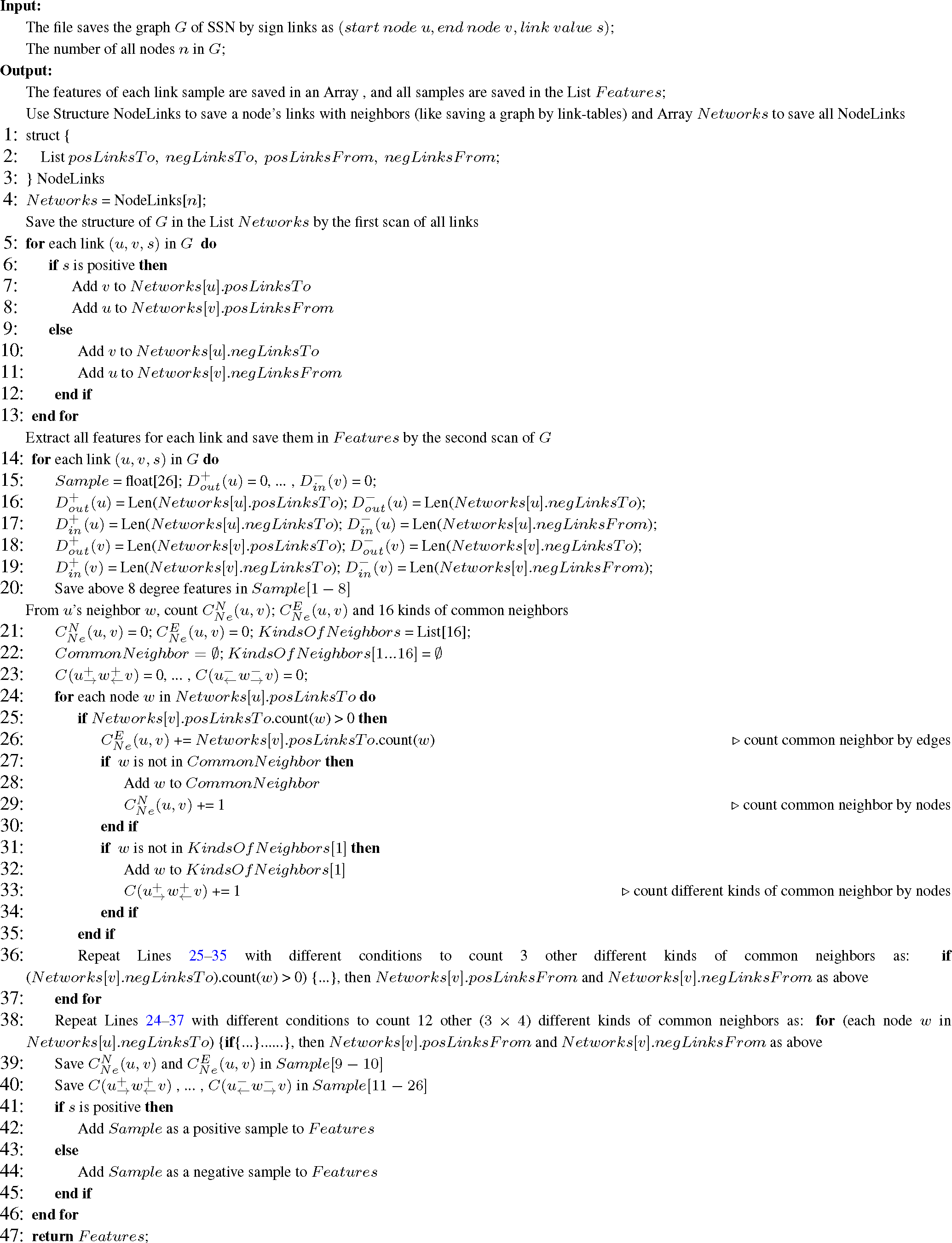The details are shown in Algorithm 1, and there are a total of 18 features that form the neighbor features.

Algorithm 1. Algorithm for extracting features from an signed social network (SSN).

Algorithm 1. Algorithm for extracting features from an signed social network (SSN).

The algorithms to extract the above features are shown in Algorithm 1. The input is the graph of the SSN saved by a set of links as (start node u, end node v, link value s), and the output is the List Features that contains each link’s features saved in an Array. The main strategy of the algorithm is based on scanning the graph by links two times: the first time, the NodeLinks Structure Array Networks contains the whole structure of which the graph is built; the second time, each link’s features are extracted and added to the List Features. In order to speed up the procedure of extracting features, the data structure NodeLinks with four Lists are used to save links for each node. Those lists contain both links that started from this node and ended with that node and separated by positive and negative values. For example, Networks[u].posLinksTo saves all of the positive links starting with node u, and Networks[v].negLinksFrom saves all of the negative links ending with v. Therefore, this algorithm needs 2 × n(n = number of links) random access memory (RAM) to save the graph Networks and O(n) time to build the Array Networks. However, the storage cost makes it possible to count the 8 degree features in linear O(n) time, because it does not need to scan the whole graph to find all of the links ending with a node, and it would cost O(n²) if only the links that started from this node were saved. When counting the 18 neighbor features, the time cost is O(n + m²)(m = max number of neighbors for each node), because the algorithm needs m × m steps to find all kinds of common neighbors that are shared by two nodes. As a result, the total time cost of this algorithm is O(n + m²), and it needs 2 × n RAM space.

4.2. Unsupervised Link Prediction

Hinton and Salakhutdinov show the ability of DBN-based autoencoders in [28]. They get two-dimensional codes of images by a 784-1000-500-250-2 (DBN with 4 RBMs and their dimensions (visible × hidden) as 1st (784 × 1000), 2nd (1000 × 500), 3rd (500 × 250) and 4th (250 × 2)) autoencoder and two-dimensional codes of documents by a 2000-500-250-125-2 (DBN with 4 RBMs and their dimensions (visible × hidden) as 1st (2000 × 500), 2nd (500 × 250), 3rd (250 × 125) and 4th (125 × 2)) autoencoder. The visualization results show that the autoencoder works better than using PCA (principal components analysis) to reduce the dimensionality of data, and the results are like the ones by the clustering method. That inspired us to use DBN to encode the link feature’s for link prediction and to use the code as the “value” of that link.

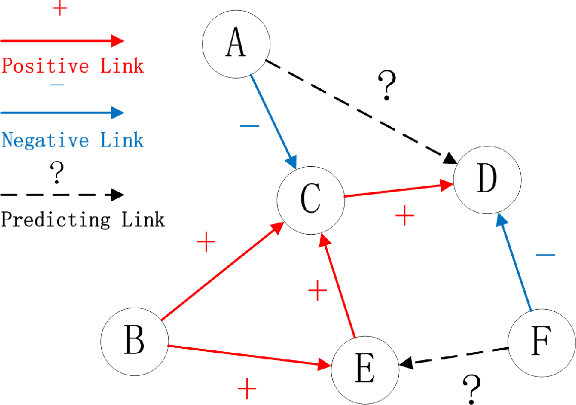
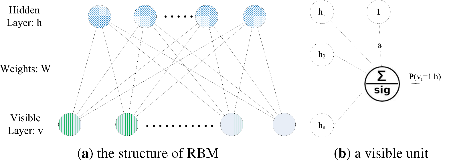
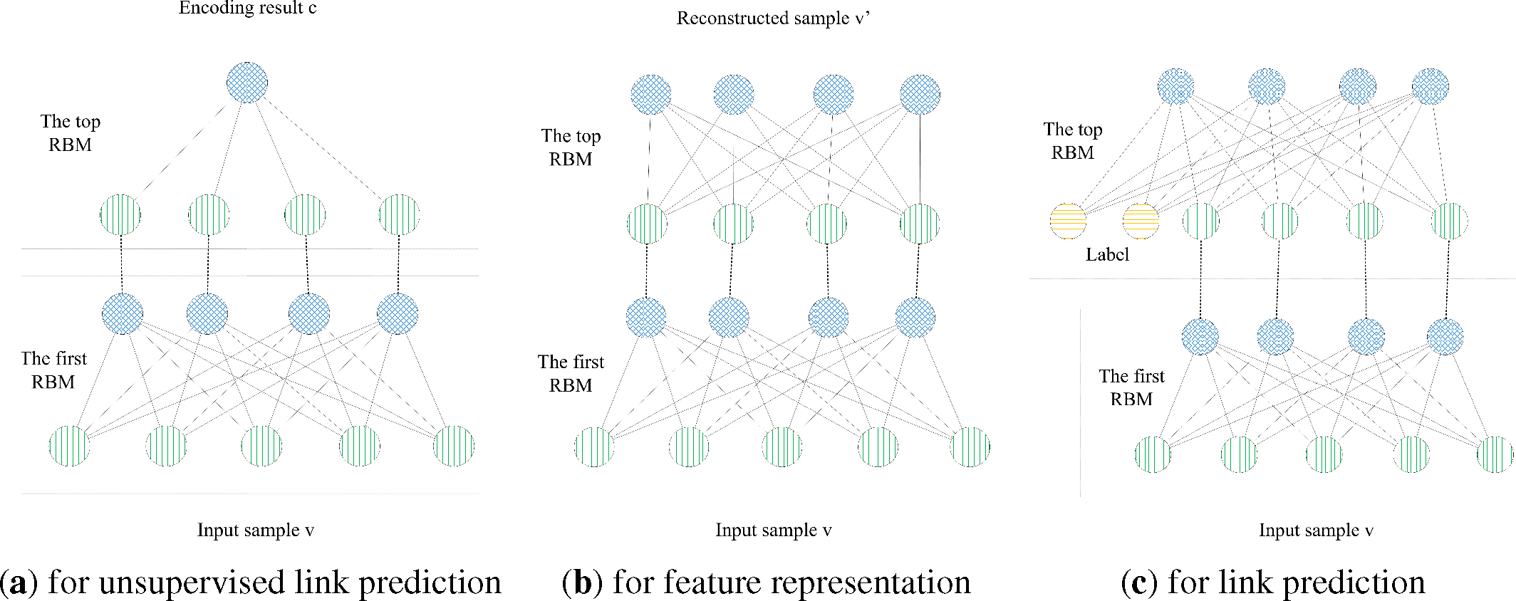
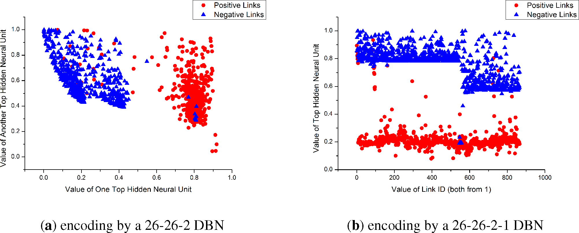
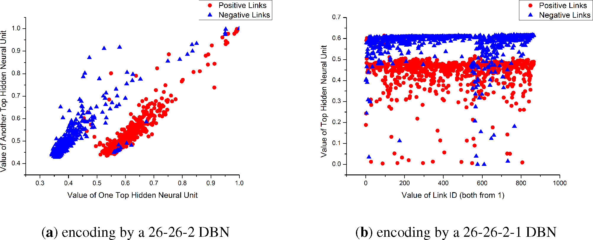
To train a model for unsupervised link prediction, We use a DBN with the structure as shown in Figure 4a. Through all RBMs, the dimension of the input sample vector is decreased. Though a 26-26-2 DBN with 2 RBMs—1st (26 × 26) and 2nd (26 × 2)—as shown in Figure 5a, we found that the two-dimensional code from the DBN could represent the “meaning” of samples properly. Because there are two classes of link values (positive and negative) in our problem, we try to use one-dimension to represent the sample’s label. If the last hidden layer has one neuron, whose output (one-dimensional code) could be treated as a probability value to be zero or one, we can take the probability value as how it belongs to a class label. Such a method is similar to Hinton’s, so the one-dimensional code could stand for the “value” of the link sample, by which the code is generated.

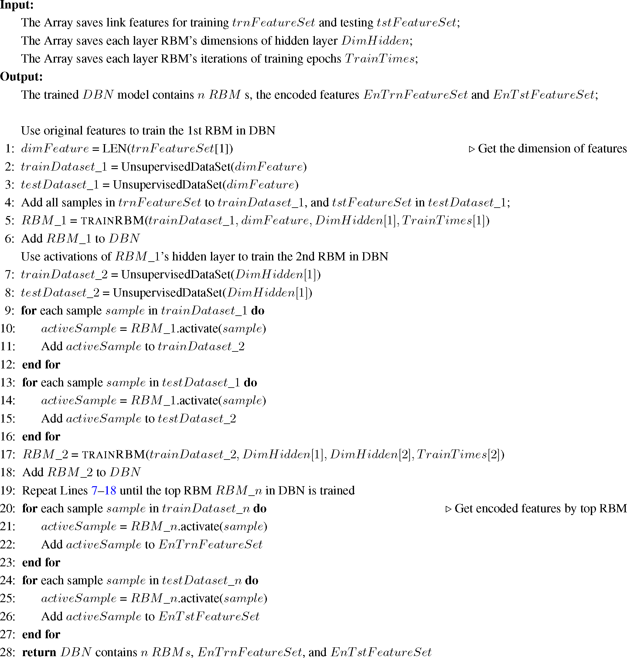
With a continuous value, the one-dimensional code could represent the abstracted label of the input sample. This method works like a clustering method that “clustering” each sample to a real value in [0, 1], and the value means to which class the sample should belongs. As shown in Figure 5b, samples with different kinds of links have different top hidden unit values. The details of this method are shown in Algorithm 2. In order to get one one-dimensional code, the DimHidden = [26,1] and TrainTimes = [50,50]. The code of each sample in tstFeatureSet is saved in EnTstFeatureSet. Then, we normalize the code values in EnTstFeatureSet by a sigmoid function and make the evaluations.

Algorithm 2. Algorithm of building a deep belief network (DBN) for unsupervised link prediction.

Algorithm 2. Algorithm of building a deep belief network (DBN) for unsupervised link prediction.

4.3. Feature Representation

Well-trained RBMs have high representation power. Bengio and Courville suggest training the representation of features by deep networks firstly for several tasks in [27]. That inspired us to use RBMs to represent the link prediction features and to use the represented features as the input for training another classifier.

We use the DBN as shown in Figure 4b to represent the link prediction features. The original feature vectors are used as the first RBM’s visible units’ input. Then, we activate each layer of the network and use the top RBM’s hidden units’ output as the represented feature vectors. After this process, we use the represented features to train a logistic regression model introduced by Jeffrey Whitaker [38] to classify link values.

The details of this method are shown in Algorithm 3. The original features are saved in trnFeatureSet and tstFeatureSet, and the features that are represented by the DBN are saved in repTrnFeatureSet and repTstFeatureSet. Then, the samples in repTrnFeatureSet are used as the dataset to train a logistic regression model, and the repTstFeatureSet is used as the test dataset to evaluate the method’s performance.

4.4. DBN-Based Link Prediction

A DBN is used to recognize handwritten digit images with high accuracy in [17]. The DBN with RBMs forms a very good generative model that represents the joint distribution of handwritten digit images and their labels. That inspired us to use a similar method to get the joint distribution of link samples and their sign values.

Algorithm 3. Algorithm for building a DBN for feature representation.

Algorithm 3. Algorithm for building a DBN for feature representation.

We use a DBN as shown in Figure 4c. In order to get the input vector for the top RBM’s visible layer shown in Figure 4c, we need to construct a vector that combines a link’s sample and its label. Firstly, we transform the link value label to a binary class label vector. The dimension of each label vector is the same as the many classes we have in the dataset. The detail is setting all label vector bits to “0”, then only setting the i-th bit to “1”, if the sample belongs to the i-th class. At the same time, we represent the samples by the above feature representation method. Then, we join the represented sample vector with that sample’s binary class label vector as the input visible vector for training the top RBM. Because the RBM can learn the distribution of all input visible vectors, the top RBM could model the joint distribution of represented link samples and their labels. When predicting a sample’s label, we use the following method.

After training the top RBM, a represented sample is joined with each possible binary class label vector as the input for the top RBM, and we get a set of free energy for each combination by:

$$F(v)=-{\displaystyle \sum _i{v}_i{a}_i-{\displaystyle \sum _j\log (1+e^{h_j})}}$$

(3)

where v_i is the value of visible unit i and a_i is v_i’s bias; h_j is calculated by Equation (1)

For example, there is a sample s. We firstly get the representation of the sample s by the bottom RBMs and denote that vector as v. Then, we combine v with each binary class label {c₁, c₂…c_i…} and get a set of possible combine vectors as {vc₁, vc₂, …vc_i….}. After inputting each of them into the top RBM, a set of free energy {F(vc₁), F(vc₂), …F(vc_i)…} for these possible combined vectors can be obtained by Equation (3). Then, we can use a SoftMax method as:

$$\log P(label=c_i|v)=\frac{e^{-F(v{c}_i)}}{{\displaystyle \sum _j{e}^{-F(v{c}_j)}}}$$

(4)

to get the log probability of which class label the vector v (sample s) should have.

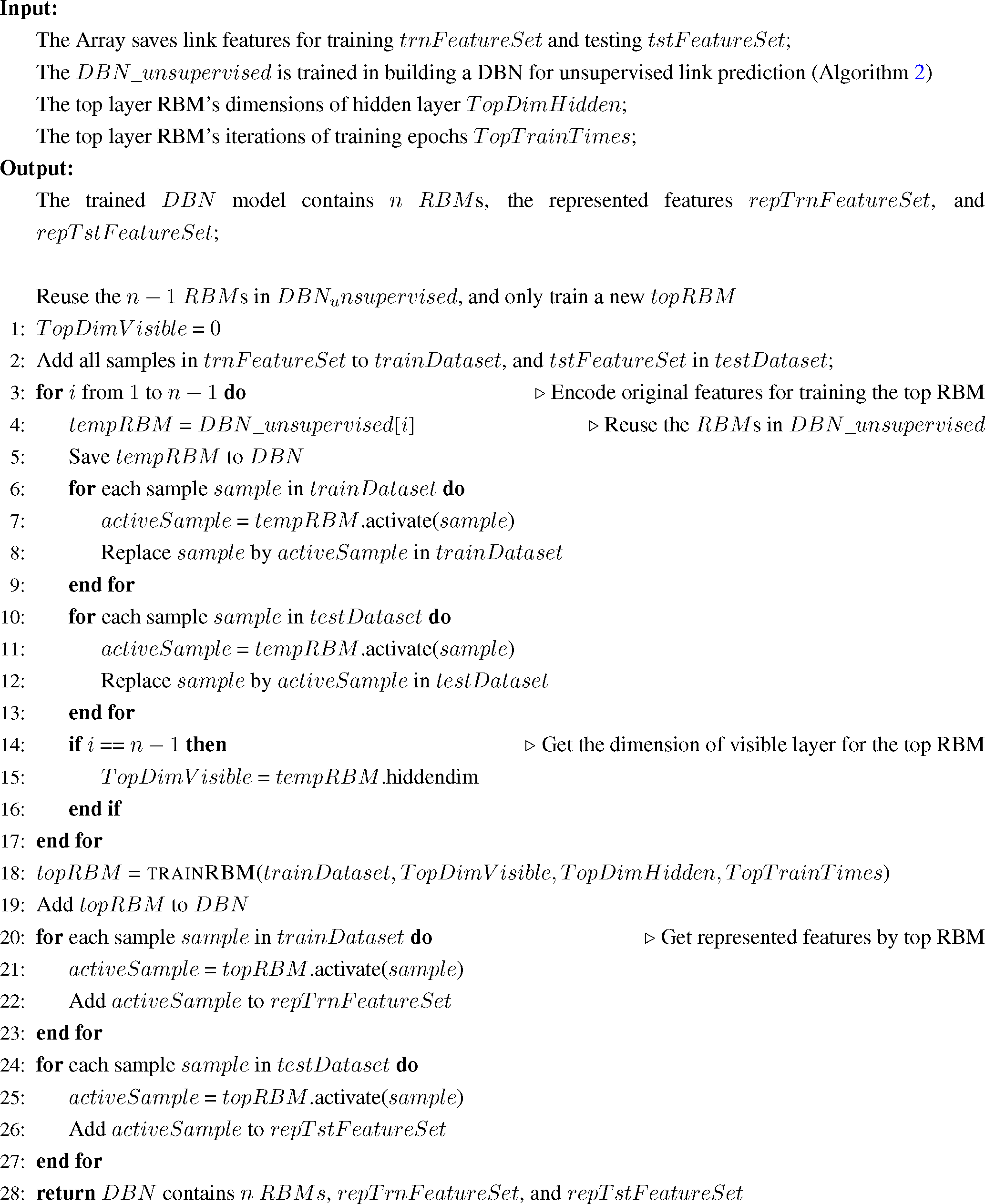
The details of this method are shown in Algorithm 4. The repTrnFeatureSet and repTstFeatureSet contain the represented samples. As shown in Algorithm 4, Lines 7–17, use repTrnFeatureSet to make the training dataset trainDataset for the top RBM and use repTstFeatureSet to make the possible test datasets assumePosTestDataset and assumeNegTestDataset. Then, use the trained top RBM to get all free energy with the test datasets by Equation (3) in Algorithm 4, Lines 20–26 and save them assuming as a positive class assumePosFreeEnergySet and assuming as a negative one assumeNegFreeEnergySet. Finally, use assumePosFreeEnergySet and assumeNegFreeEnergySet to get the probability for each sample’s class label by Equation (4).

4.5. Training Strategy

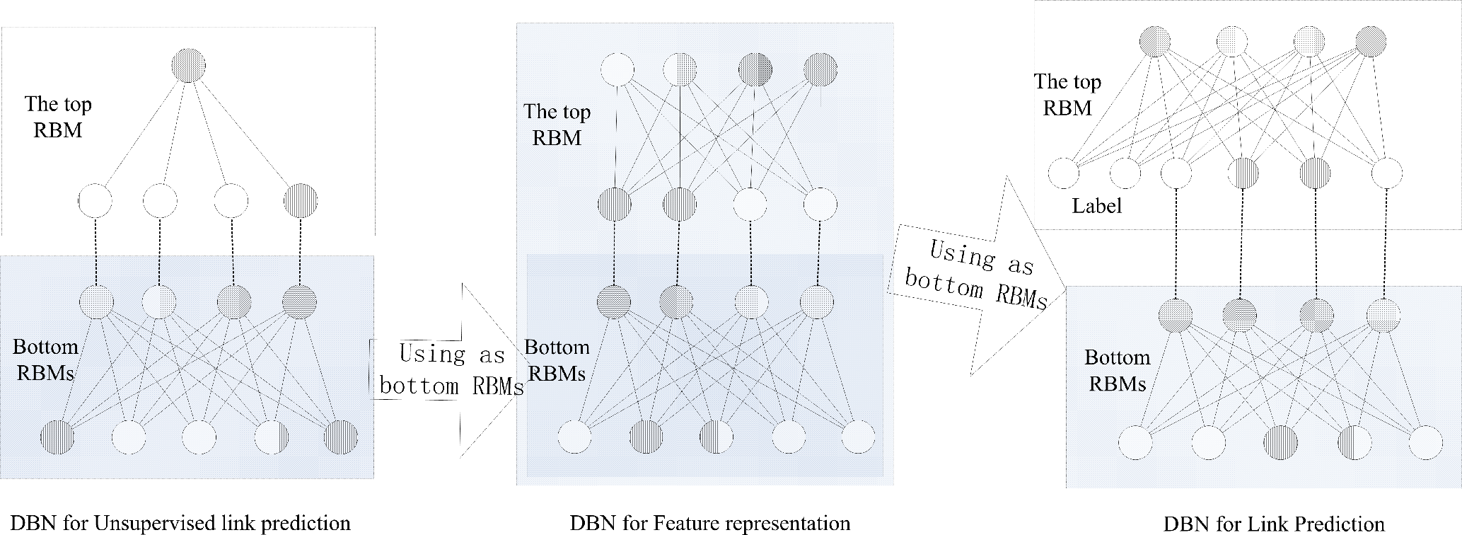
Training the DBN is a time-consuming task, because a well-trained RBM needs lots of iterations before convergence. If we train DBNs for more than three tasks independently, it would cost a lot of time and we would have to check whether all RBMs are well trained. We design a strategy to reuse RBMs as shown in Figure 6. Such a learning strategy can save a lot of training time and allow us to check whether these methods are suitable for the problem early on by the experiment results of the first methods.

Algorithm 4. Algorithm for building a DBN for DBN-based link prediction.

Algorithm 4. Algorithm for building a DBN for DBN-based link prediction.

Firstly, we have no trained RBMs, so we build the DBN for unsupervised link prediction with newly-trained RBMs. We train each RBM individually; the first RBM is trained by the original features. After finishing training of the first RBM, the second RBM is trained by the output of the first RBM’s hidden vectors, which are generated by the original features. Repeat this process until finishing the training of the top RBM. Therefore, the DBN is trained for unsupervised link prediction. Secondly, we start to build up the DBN for the feature representation method. Except the top RBM, we take the bottom RBMs trained for unsupervised link prediction as the bottom RBMs in the DBN for feature representation. Then, we train the top RBM by the hidden vectors’ activities from the bottom RBMs. Thirdly, when we build up the DBN for DBN-based link prediction method, we take the whole DBN for feature representation as the bottom RBMs. Additionally, we train the top RBM by the method introduced in Section 4.4.

By reusing the trained DBN’s RBMs, the cost of building the next DBN only requires the time cost of training a new top RBM. Anyway, those methods are more suitable for a static environment than an online environment. The main reason is that the DBNs need to be trained step by step with enough balance samples at the beginning. As introduced in Section 3.2, the RBM is trained by an unsupervised process. If the samples are not balanced, it would cause modeling the larger prediction error at the beginning. Additionally, the error would be difficult to fix, for the learning process is unsupervised. In an online environment, it would be very difficult to keep the balance of samples with different labels at the beginning. As a result, we advise building up these DBNs in a static environment; then, one can use it for some online systems. When one wants to update these models for later usage, we also advise rebuilding these DBNs with new samples and replacing the old DBNs.

4.6. Generalization Across Datasets

In order to check whether the above methods are suitable for common datasets from SSNs, we test the model generated across datasets. If the trained models can generalize across datasets properly, this suggests that there are underlying general principles that guide the creation of links in an SSN, and our method could obtain this.

Shown in Figure 7 is the result of the same testing dataset as shown in Figure 5, while the DBN is trained from another training dataset. Although the results are not as good as the ones in Figure 5, this shows that the DBN trained from the other dataset could also encode link features with acceptable performance. The main difference is the value scale of the top hidden units as shown by the range of the axis. Similarly, the DBN trained on the same dataset would have better hidden unit value distributions than the DBN trained from another dataset.

5. Experimental Introduction

This section includes the introduction of the datasets used in our study, our experimental setup and the evaluation metrics.

5.1. Dataset Description

In this paper, three datasets from different social networks are used. They are available online in the Stanford Large Network Dataset Collection ( http://snap.stanford.edu/data/). The datasets are individually from the websites Wikipedia, Slashdot and Epinions. All of the links in the above datasets are explicitly positive or negative. The data from Wikipedia are about the votes for Wikipedia admin role promotion; Slashdot’s data are from Slashdot Zoo, which allows users to tag each other as “friends” or “foes”; Epinions is a product review website, whose data are about whether users trust each other’s comments on goods.

In the datasets (Epinions, Slashdot and Wikipedia), using sign value “+1” stands for “agree”, “friend” and “support”, while value “−1” stands for “disagree”, “foe” and “oppose”. In many social networks, one user could show their attitude toward another user more than once, so there may be several edges with the same or different sign values and directions between two nodes.

It is well known that the three websites (Wikipedia, Epinions and Slashdot) are typical kinds of social networks. The node’s degree distribution of each dataset is shown in Figure 2, where the curves are mainly linear and which accords with the complex network’s degree power law distribution. In the Wikipedia promotion dataset, nearly 60% of the nodes have 1 to 10 degrees and over 90% of the nodes have degrees less than 100. The Epinions and Slashdot datasets have nearly the same degree distribution as Wikipedia’s.

There is another common phenomenon among these datasets, that is the distribution of the links’ sign value is imbalanced. Over 75% percent of links are positive in all datasets. Especially in Epinions’ dataset, there are 85% of links with positive sign values. This distribution of data may cause modeling the larger prediction error, which classifies links more likely to the class with more samples. In order to avoid this problem for unsupervised learning, we lost positive links randomly until the two classes became balance. Then, we randomly selected a start node and get the largest connection graph started from that node. If there are less than 5000 links in that graph, we will select another start node and add another biggest connection graph started from that node until there are at least 5000 links in the network. Then, we extract the features, introduced in Section 4.1, from that network as the link samples. In order to make these features suitable as the input for the visible layer of the RBM, we normalize each feature to the range [0,1] and treat it as a continues value. In the following experiments, 80% of the data is used as the training set, and the other 20% is used as the testing set.

5.2. Experimental Setup

In our experiments, the toolkit PyBrain (version 0.31) ( http://pybrain.org/) is used. As introduced in [39], PyBrain is a versatile machine learning library for Python. Its goal is to provide flexible, easy to use, yet still powerful algorithms for machine learning tasks, including a variety of predefined environments and benchmarks to test and compare algorithms. PyBrain is achieved by the Python language. It provides a well-designed data structure to save training and testing datasets, and its trainer RbmBernoulliTrainer is based on the CD algorithm introduced by Hinton [36].

The parameters, such as training rate, training times and iteration times for Gibbs sampling, affect the models’ performance greatly. It seems impossible to try every combination of them, for that will cost much time. However, there is a common theme of how to set them up to train a RBM. The most determining factor is the dimensions of the RBM’s visible and hidden layers. If the hidden layer’s dimension is higher than the visible layer’s, the iteration times for Gibbs sampling should be set to a higher value. While in the opposite condition, the iteration times should be set to a lower value. We could find basic reference values of these parameters when training the first RBM.

For training an RBM, the detail are shown in Algorithm 5. There are dimVis × dimHid weights and dimV is + dimHid biases to be learned in the algorithm. To learn those weights and biases, all of the samples in trainData are used to modify these by the CD algorithm in each training epoch. Additionally, trainTimes training epochs are performed. We can assume the time cost based on how much time the CD algorithm costs. The CD algorithm is based on the BP (back propagation) algorithm, the difference being that it uses Gibbs sampling. Therefore, the CD algorithm’s cost is O(c × (BP)), and the cost of BP is determined by how many weights and biases are to be learned. For training a DBN, the number of RBMs that need to be trained is shown in Algorithms 2–4. As a result, the time cost of the DBN is O(c × (RBM)).

In our condition, we use a PC with Intel Xeon 2.0 GHz and 6 GB RAM to train an RBM. It would cost about 4–5 min to train a bottom RBM with dimensions of 26 × 26 with 4000 samples in trainData and trainTimes as 50. When the dimensions increase, the trainTimes should also increase. Therefore, we train the RBM with dimensions of 26 × 52 or (2 + 26) × 52 with trainTimes as 100. It would take about 14–15 min to finish training such an RBM. The time cost of finishing the training of the DBN would be about 10 min for Algorithm 2 with two RBMs, another 15 min to add a top RBM for Algorithm 3 and another 15–30 min to add a top RBM for Algorithm 4. During the training process, at most about 2 GB RAM is needed.

Algorithm 5. Algorithm for training an RBM by PyBrain.

Algorithm 5. Algorithm for training an RBM by PyBrain.

5.3. Evaluation Metric

There are several performance measures for multi-label evaluation introduced by Nowak et al. in [40]. In order to evaluate the above methods properly, we will use the following metrics. First of all, precision for each class is used as an evaluation measure. Secondly, the binary classification problem can be treated as a detection problem, and we compute each classes’s F1 score to show our method’s ability. Thirdly, the receiver operating characteristic (ROC) curve, which is introduced by Fawcett in [41], is often used as the measure of detection performance. Based on the ROC curve, the area under the curve (AUC) for each class is used as an evaluation measure.

5.4. Comparison with the Similarity-Based Method

As shown in Section 4, our methods are based on statistics techniques and machine learning approaches. In order to make a more complete comparison with other state-of-the-art link prediction methods, we also use the FriendTNS± introduced by Symeonidis and Tiakas in [26]. The FriendTNS± is based on transitive node similarity, which calculates the similarity of two indirectly connected users by using their shortest path by following:

$$esim(v_i,v_j)=\{\begin{array}{cc}0& \text{if there is no path between}{v}_i,v_j\\ sim(v_i,v_j)& \text{if}{v}_i,v_j\text{are neighbours}\\ {\displaystyle \prod _{h=1}^{k}sim(v_{ph},v_{ph+1})}& \text{otherwise}\end{array}$$

(5)

where v_p1 = v_i, v_pk+1 = v_j and the nodes v_ph (for h = 2, …, k) are all of the intermediate nodes through which the shortest path from v_i to v_j passes.

We choose this similarity-based method as one comparison because the neighbors’ similarity sim(v_i, v_j) in Equation (5) can be extending for an SSN. Different from most other similarity-based algorithms only considering positive links, the FriendTNS± also considers the negative links in an SSN by following:

$$sim(v_i,v_j)=\frac{1}{\partial (v_i)+\partial (v_j)-1}$$

(6)

where $\partial (u)=D_{in}^{+}(u)+D_{out}^{-}(u)-D_{out}^{+}(u)-D_{in}^{-}(u)$ and the degrees are defined in Section 4.1.

However, like other similarity-based methods, the FriendTNS± algorithm aims to recommend top k friends for one user (problem of predicting the existence of a link). It is somewhat different from our work that aims to classify users’ relationships (problem of predicting the sign value of a link). In order to make a direct comparison, we need to change the FriendTNS± algorithm’s evaluation metric introduced in the original article [26]. For one user u in the network, the original evaluation metric is to check it as a recommended method; that is, whether the users who have the top k similarity would have a link with user u, which is similar to predicting positive links for user u. This evaluation is not so suitable an evaluation metric for the problem of predicting the sign value of a link, because the negative links also need to be predicted in our problem. Therefore, we make some changes that make the evaluation more suitable for a multi-label classification problem than the original one as follows.

First of all, we do not make any change in the FriendTNS± algorithm, but in the evaluation. Secondly, for one user u, we use the FriendTNS± to get all of the similarities between u and the users who have a link with u. Then, we select the top k similarities from both positive links and negative links, so we get 2k samples that each have a similarity and a certain sign value. Thirdly, we treat the 2k samples, k positive ones and k negative ones, as a multi-label classification problem based on their similarities. This means that we check whether the link’s sign value could be classified just by its similarity value. Finally, we could use the evaluations introduced in Section 5.3 to show the FriendTNS±’s ability at predicting the sign value of links. We select three k values (5,10,20) in this experiment, and k is set to MIN(numberofpositivelinkofu, numberofnegativelinkofu) when node u does not have at least k positive links or negative links. The experiment result is shown in Section 6.1 for this algorithm; it does not need to know the link value when calculating the linked nodes’ similarities, which point looks like the unsupervised learning.

6. Experimental Results and Analysis

In this section, the results of our methods, unsupervised link prediction, feature representation and DBN-based link prediction are introduced separately in the following three subsections. Additionally, the results of the generalization across datasets experiment are listed separately following each method’s result in each subsection.

All of the experiment results are shown in tables. Each table can be divided into five columns. The first column contains the DBN structure when showing each of the three method’s results; while, the first column becomes the name of the training dataset when showing the result of the generalization across the dataset experiment. The second, thirds and fourth column contains the experimental results on the testing set from the Wikipedia, Epinions and Slashdot dataset. The fifth column is the average value of the second, third and fourth columns. The first row in each table is the name of the testing dataset and the metrics, except the first unit. Each of the following rows is the result of a certain network structure or method.

6.1. Results for Unsupervised Link Prediction

The results of the unsupervised link prediction are shown in

Table 1. Result for the unsupervised link prediction (positive class).

Methods	Wikipedia			Epinions			Slashdot			Average
	Precision	F1 score	AUC	Precision	F1 score	AUC	Precision	F1 score	AUC	Precision	F1 score	AUC
FriendTNS ±
FriendTNS± (Top 5)	0.7747	0.7585	0.8679	0.7589	0.7597	0.8634	0.7813	0.7663	0.8762	0.7716	0.7615	0.8692
FriendTNS± (Top 10)	0.7012	0.6773	0.7849	0.6762	0.6798	0.7722	0.7053	0.6923	0.7977	0.6942	0.6831	0.7849
FriendTNS± (Top 20)	0.6464	0.6215	0.7165	0.6141	0.6231	0.6923	0.6555	0.6465	0.7361	0.6387	0.6304	0.7150
DBN with two RBMs
1st (26 × 13) 2nd (13 × 1)	0.7321	0.5524	0.7574	0.6278	0.7422	0.8170	0.6775	0.7099	0.7707	0.6791	0.6682	0.7817
1st (26 × 26) 2nd (26 × 1)	0.7700	0.6496	0.8025	0.8386	0.7631	0.8647	0.7400	0.7748	0.8138	0.7829	0.7292	0.8270
1st (26 × 52) 2nd (52 × 1)	0.7630	0.7026	0.7742	0.8036	0.7449	0.8537	0.6163	0.7107	0.7068	0.7276	0.7194	0.7782

(positive class) and

Table 2. Result for the unsupervised link prediction (negative class).

Methods	Wikipedia			Epinions			Slashdot			Average
	Precision	F1 score	AUC	Precision	F1 score	AUC	Precision	F1 score	AUC	Precision	F1 score	AUC
FriendTNS±
FriendTNS± (Top 5)	0.7531	0.7682	0.8678	0.7600	0.7592	0.8636	0.7609	0.7749	0.8763	0.7580	0.7674	0.8692
FriendTNS± (Top 10)	0.6763	0.6979	0.7850	0.6801	0.6764	0.7724	0.6909	0.7032	0.7977	0.6824	0.6925	0.7850
FriendTNS± (Top 20)	0.6262	0.6486	0.7166	0.6211	0.6118	0.6924	0.6473	0.6559	0.7361	0.6315	0.6383	0.7150
DBN with two RBMs
1st (26 × 13) 2nd (13 × 1)	0.6007	0.6997	0.7574	0.8332	0.5946	0.7782	0.7172	0.6792	0.7766	0.7170	0.6578	0.7707
1st (26 × 26) 2nd (26 × 1)	0.6552	0.7332	0.7956	0.7426	0.7993	0.8518	0.7926	0.7514	0.8138	0.7301	0.7613	0.8204
1st (26 × 52) 2nd (52 × 1)	0.6958	0.7433	0.7636	0.7309	0.7775	0.8532	0.7483	0.5829	0.7119	0.7250	0.7012	0.7763

(negative class). The first three rows are the results of FriendTNS± with different k values, as introduced in Section 5.4, and the last three rows are the results of our unsupervised link prediction. Two-layer RBMs are used in our method, and their structures are listed in the first column. The first numbers (1st, 2nd…) stand for which layer the RBM is in, and the dimension of that RBM’s visible layer and hidden layer is listed as (visible dimension × hidden dimension). Because there are 26 features in one sample, the first RBM has a visible layer with 26 units. Because the structure of the RBM affects the performance greatly, we try three different RBMs with hidden layer dimensions of 13, 26 and 52. The second RBM’s visible layer should have the same dimensions as the first RBM’s hidden layer, and its hidden layer has one unit, whose value stands for to what the input vector should belong. The result of each DBN model is listed in one row in these tables.

First of all, all of the results show that the two method can predict link values properly. The performance of FriendTNS± is very good when k is small, but it drops a lot when k becomes large. The result shows that the link with a high similarity of linked nodes is more likely to be a positive one than the link with low similarity. As k become larger, more links with not so high similarity are predicted as positive, while more links with not so low similarity are predicted as negative. In this condition, judging the links only based on similarity becomes not very effective. That is, there are more links with different sign values having not so distinguishable similarities, which causes the performance of FriendTNS± to drop. Anyway, it is a good algorithm with good performance and low computing time and memory space.

Secondly, the unsupervised link prediction could encode link features without knowing the training samples’ labels. The average values show that both “positive” and “negative” classes could be detected with acceptable performance; although, the precision and F1 score varies a lot for different class, while the AUC value is nearly unchanged, and this means that all classes can be detected properly. By analyzing the metrics’ variances between rows, we find that the structure of each layer of the RBM affects the performance greatly. In order to find a suitable network structure, we tried three different RBMs with hidden layer dimensions of 13 (half of the feature’s dimension), 26 (same as the feature’s dimension) and 52 (double the feature’s dimension). From the average of the metric values, it is shown that the DBN structure with the first RBM of 26 × 26 and the second RBM of 26 × 1 performs the best in these three, and the structure with the first of 26 × 13 and the second of 13 × 1 works worsts. This shows that sharply reducing the feature’s dimension by the first RBM is not good, because doing that may cause the loss of some useful information contained by the input vectors.

The DBN structure with the first of 26 × 52 and the second of 52 × 1 dose not perform best, though it is the most complex one of these three. We checked the hidden vectors from the first RBM and found that the outputs with a dimension of 52 were much more sparse than the ones with 26 dimension; while the second RBM (52 × 1) may not have the ability to summarize such a sparse input vector properly. As a result, the combination of the first RBM (26 × 26) and the second RBM (26 × 1) becomes the most suitable one for this task.

The experiment of the generalization across datasets for the unsupervised link prediction is based on the network structure with the first RBM of 26 × 26) and the second RBM of 26 × 1, whose performance is best for unsupervised link prediction. The results are shown in

Table 3. Results for unsupervised link prediction across datasets (positive class).

Test Data	Wikipedia			Epinions			Slashdot			Average
Train Data	Precision	F1 score	AUC	Precision	F1 score	AUC	Precision	F1 score	AUC	Precision	F1 score	AUC
Wikipedia	0.7700	0.6496	0.8025	0.7763	0.6994	0.8276	0.6656	0.6932	0.7124	0.7373	0.6807	0.7808
Epinions	0.6527	0.5617	0.7440	0.8386	0.7631	0.8647	0.6596	0.4580	0.6924	0.7170	0.5943	0.7670
Slashdot	0.6889	0.6485	0.7089	0.6745	0.7204	0.7784	0.7400	0.7748	0.8138	0.7011	0.7146	0.7670

(positive class) and

Table 4. Results for unsupervised link prediction across datasets (negative class).

Test Data	Wikipedia			Epinions			Slashdot			Average
Train Data	Precision	F1 score	AUC	Precision	F1 score	AUC	Precision	F1 score	AUC	Precision	F1 score	AUC
Wikipedia	0.6552	0.7332	0.7956	0.6919	0.7491	0.8272	0.6969	0.6367	0.7207	0.6813	0.7063	0.7812
Epinions	0.5928	0.6574	0.7113	0.7426	0.7993	0.8518	0.5578	0.6636	0.6445	0.6311	0.7067	0.7359
Slashdot	0.6511	0.6853	0.6898	0.7343	0.6763	0.7168	0.7926	0.7514	0.8138	0.7260	0.7043	0.7402

(negative class). The first column is the names for the training datasets, and in the second, third and fourth columns are the results on testing datasets from the three different websites. There is no cover between training datasets and testing datasets. The fifth is the average value of the above three columns.

The results show that our method has good generalizing ability across these datasets. We find that each testing dataset’s best result is obtained by the model trained by its own training dataset. As shown in Figures 5 and 7, all of the testing dataset is from Epinions, while the training dataset is from Epinions (Figure 5) and Slashdot (Figure 7). The difference is caused by the different interest of these SNS, so the encoded features distribution is different. However, the results show that if we could learn from one of these SSNs, we would do unsupervised link prediction in another.

6.2. Results for Feature Representation

The results of the feature representation are shown in

Table 5. Result for feature representation (positive class).

Methods	Wikipedia			Epinions			Slashdot			Average
	Precision	F1 score	AUC	Precision	F1 score	AUC	Precision	F1 score	AUC	Precision	F1 score	AUC
Logistic Regression	0.8310	0.8199	0.8791	0.9019	0.8466	0.9442	0.7813	0.8255	0.8949	0.8380	0.8307	0.9061
DBN with two RBMs
1st (26 × 26) 2nd (26 × 13)	0.8471	0.7905	0.8773	0.8983	0.8875	0.9460	0.8267	0.8466	0.9075	0.8574	0.8416	0.9103
1st (26 × 26) 2nd (26 × 26)	0.8574	0.8160	0.9055	0.9478	0.9284	0.9572	0.8998	0.9048	0.9531	0.9017	0.8831	0.9386
1st (26 × 26) 2nd (26 × 52)	0.8604	0.8221	0.9087	0.9292	0.8811	0.9601	0.8943	0.9074	0.9601	0.8932	0.8719	0.9449

(positive class) and

Table 6. Result for feature representation (negative class).

Methods	Wikipedia			Epinions			Slashdot			Average
	Precision	F1 score	AUC	Precision	F1 score	AUC	Precision	F1 score	AUC	Precision	F1 score	AUC
Logistic Regression	0.8149	0.8254	0.8791	0.8184	0.8631	0.9441	0.8580	0.8032	0.8949	0.8304	0.8306	0.9060
DBN with two RBMs
1st (26 × 26) 2nd (26 × 13)	0.7701	0.8154	0.8773	0.8798	0.8901	0.9460	0.8606	0.8389	0.9075	0.8368	0.8481	0.9103
1st (26 × 26) 2nd (26 × 26)	0.7973	0.8324	0.9055	0.9132	0.9312	0.9494	0.9089	0.9037	0.9531	0.8731	0.8891	0.9360
1st (26 × 26) 2nd (26 × 52)	0.8040	0.8368	0.9087	0.8522	0.8918	0.9448	0.9186	0.9048	0.9601	0.8611	0.8782	0.9398

(negative class). The first row is the result of the logistic regression model trained with original features, and we take it as the baseline measure. The following rows are the result of the logistic regression model trained with the represented features. The DBN structure is listed in the first column, and the dimensions are expressed as (visible × hidden). We use the same bottom RBMs trained in the unsupervised link prediction experiment. Because the first RBM’s structure is (26 × 26), the second RBM has a layer visible with 26 units. We also try three different second RBM’s structures with hidden layer dimensions of 13, 26 and 52. The result of each DBN model is listed in one row in these tables.

The results show that logistic regression performs better when the model is trained by represented features rather than original features. Although the represented feature’s dimension is reduced to 13 (half of the original feature’s dimension), the average measures are not worse than the baseline. This shows that reducing the dimension of the features that have been represented by bottom RBMs is available in higher RBMs. When the represented feature’s dimension increase to 26 (the same as the original feature’s dimension), the performance of the link prediction is improved. This shows that the represented features could better express the meaning of the samples, and our method for feature representation works well.

When raising the represented feature’s dimension up to 52 (double the original feature’s dimension), though it costs much more time to train the top RBM, the results are not improved much more than the RBM with 26 hidden units. We checked the activation of that model’s hidden vector and found that it is much sparser than the 26-dimension RBM’s. This shows that 26 dimensions are nearly large enough for representing link prediction features. Therefore, it may be the most suitable DBN structure for this task.

The experiment of the generalization across datasets for feature representation method is based on the logistic regression (LR) model trained with the features that are represented by the network structure with the first RBM of 26 × 26 and the second RBM of 26 × 26. The results are shown in

Table 7. Results for feature representation across datasets (positive class).

Test Data	Wikipedia			Epinions			Slashdot			Average
Train Data	Precision	F1 score	AUC	Precision	F1 score	AUC	Precision	F1 score	AUC	Precision	F1 score	AUC
Wikipedia	0.8574	0.8160	0.9055	0.9322	0.8833	0.9428	0.8858	0.8752	0.9332	0.8918	0.8582	0.9272
Epinions	0.8128	0.8048	0.8891	0.9478	0.9284	0.9572	0.8809	0.8819	0.9420	0.8805	0.8717	0.9294
Slashdot	0.7885	0.8018	0.8721	0.8445	0.8704	0.9293	0.8998	0.9048	0.9531	0.8443	0.8590	0.9182

(positive class) and

Table 8. Results for feature representation across datasets (negative class).

Test Data	Wikipedia			Epinions			Slashdot			Average
Train Data	Precision	F1 score	AUC	Precision	F1 score	AUC	Precision	F1 score	AUC	Precision	F1 score	AUC
Wikipedia	0.7973	0.8324	0.9055	0.8540	0.8945	0.9428	0.8680	0.8781	0.9332	0.8398	0.8683	0.9272
Epinions	0.8008	0.8085	0.8891	0.9132	0.9312	0.9494	0.8826	0.8816	0.9420	0.8655	0.8738	0.9268
Slashdot	0.8090	0.7949	0.8721	0.8910	0.8618	0.9294	0.9089	0.9037	0.9531	0.8696	0.8535	0.9182

(negative class). The first column is the names for the training datasets, and in the second, third and fourth columns are the prediction results on the three datasets. The results show that our feature representation method also has good generalizing ability across these datasets. The results show that if we could learn from one of these SSNs, we would also represent link prediction features for others.

6.3. Results for DBN-Based Link Prediction

The results of the DBN-based link prediction method are shown in

Table 9. Results for DBN-based link prediction (positive class).

Methods	Wikipedia			Epinions			Slashdot			Average
	Precision	F1 score	AUC	Precision	F1 score	AUC	Precision	F1 score	AUC	Precision	F1 score	AUC
Logistic regression learned by original features	0.8310	0.8199	0.8791	0.9019	0.8466	0.9442	0.7813	0.8255	0.8949	0.8380	0.8307	0.9061
Logistic regression with feature representation by 1st (26 × 26) 2nd (26 × 26)	0.8574	0.8160	0.9055	0.9478	0.9284	0.9572	0.8998	0.9048	0.9531	0.9017	0.8831	0.9386
DBN with three RBMs 1st (26 × 26) 2nd (26 × 26) 3rd ((26 + 2) × 52)	0.8559	0.8271	0.9146	0.9487	0.9019	0.9601	0.9054	0.9131	0.9635	0.9033	0.8807	0.9460

(positive class) and

Table 10. Results for DBN-based link prediction (negative class).

Methods	Wikipedia			Epinions			Slashdot			Average
	Precision	F1 score	AUC	Precision	F1 score	AUC	Precision	F1 score	AUC	Precision	F1 score	AUC
Logistic regression learned by original features	0.8149	0.8254	0.8791	0.8184	0.8631	0.9441	0.8580	0.8032	0.8949	0.8304	0.8306	0.9060
Logistic regression with feature representation by 1st (26 × 26) 2nd (26 × 26)	0.7973	0.8324	0.9055	0.9132	0.9312	0.9494	0.9089	0.9037	0.9531	0.8731	0.8891	0.9360
DBN with three RBMs 1st (26 × 26) 2nd (26 × 26) 3rd ((26 + 2) × 52)	0.8126	0.8382	0.9146	0.8715	0.9107	0.9601	0.9197	0.9117	0.9635	0.8679	0.8868	0.9461

(negative class). Each link prediction method’s results are listed in a row in these tables. As introduced in Section 6, we use the DBN trained in the feature representation experiment as the bottom RBMs for this task. Therefore, the top RBM’s visible layer dimension is 26 (represented feature’s dimension) + 2 (label vector’s dimension). In order to model the joint distribution of the sample and label properly, the dimension of the top RBM’s hidden layer is set to 52 (double the represented feature’s dimension).

By comparing the results of the three methods listed in the first column, our DBN-based link prediction method works better than the other two methods. The average values show that our method outperforms the baseline logistic regression method and also has improvement on the logistic regression method trained by the represented features. This shows that this method could model the joint distribution of the link samples and their labels properly, and the label could be judged by the free energies of all possible sample-label combinations through a SoftMax method.

The results of the generalization across datasets for the DBN-based link prediction method are shown in

Table 11. Results for DBN-based link prediction across datasets (positive class).

Test Data	Wikipedia			Epinions			Slashdot			Average
Train Data	Precision	F1 score	AUC	Precision	F1 score	AUC	Precision	F1 score	AUC	Precision	F1 score	AUC
Wikipedia	0.8559	0.8271	0.9146	0.9450	0.9023	0.9482	0.8974	0.8969	0.9547	0.8994	0.8755	0.9392
Epinions	0.8393	0.8099	0.8822	0.9487	0.9019	0.9601	0.8785	0.8868	0.9475	0.8888	0.8662	0.9299
Slashdot	0.8228	0.8245	0.8871	0.8891	0.8900	0.9397	0.9054	0.9131	0.9635	0.8724	0.8759	0.9301

(positive class) and

Table 12. Results for DBN-based link prediction across datasets (negative class).

Test Data	Wikipedia			Epinions			Slashdot			Average
Train Data	Precision	F1 score	AUC	Precision	F1 score	AUC	Precision	F1 score	AUC	Precision	F1 score	AUC
Wikipedia	0.8126	0.8382	0.9146	0.8741	0.9103	0.9483	0.8965	0.8970	0.9547	0.8611	0.8818	0.9392
Epinions	0.7963	0.8224	0.8822	0.8715	0.9107	0.9601	0.8932	0.8846	0.9475	0.8537	0.8725	0.9299
Slashdot	0.8254	0.8238	0.8871	0.8906	0.8897	0.9397	0.9197	0.9117	0.9635	0.8786	0.8751	0.9301

(negative class). This experiment is based on the DBN structure as the first RBM of 26 × 26, the second RBM of 26 × 26 and the third RBM of (26 + 2) × 52. The first column is the names for the training datasets, and in the second, third and fourth columns are the prediction results of the three datasets.

The results are nearly the same as the above generalization across dataset experiments, as presumed. Because the DBN in this method takes the whole DBN for feature representation as the bottom RBMs, it should inherit the above DBN’s abilities. The results show that if we could learn from one of these SSNs, we would also predict link values for other SSNs.

7. Conclusions

In this paper, the DBN-based link prediction approaches for signed social networks (SSNs) are proposed. Our strategy includes the unsupervised learning method, the feature representation and the DBN-based link predicting model. The three methods are tested on the datasets from three social networks, and the results show that they are promising for both positive and negative links in such SSNs. Additionally, they outperform the state-of-the-art methods. The generalization across datasets of these methods shows that there may exist some common hidden principles in the SSNs that drive the behaviors of social members, and our methods are able to capture them.

Our further work includes the following two directions: first, finding other methods for link prediction in SSNs; second, trying to extract more features to improve our method’s performance.