The diffusion type of distributed algorithm is not only able to respond in real time based on operating over a single time scale, but also robust to node and/or link failure [
21]. Owing to these merits, this type of distributed algorithm was widely investigated for distributed learning, such as diffusion least-mean squares (LMS) [
1,
22,
23], diffusion information theoretic learning [
5], diffusion sparse LMS [
24], diffusion recursive least-squares (RLS) [
25,
26] and diffusion sparse RLS [
27]. In this paper, we use the diffusion LMS algorithm and the diffusion RLS algorithm to adaptively adjust the output weights of the SLFN with RBF hidden neurons, which leads to the distributed ELM based on the diffusion least-mean squares (dELM-LMS) algorithm and the distributed ELM based on the recursive least-squares (dELM-RLS) algorithm, respectively.
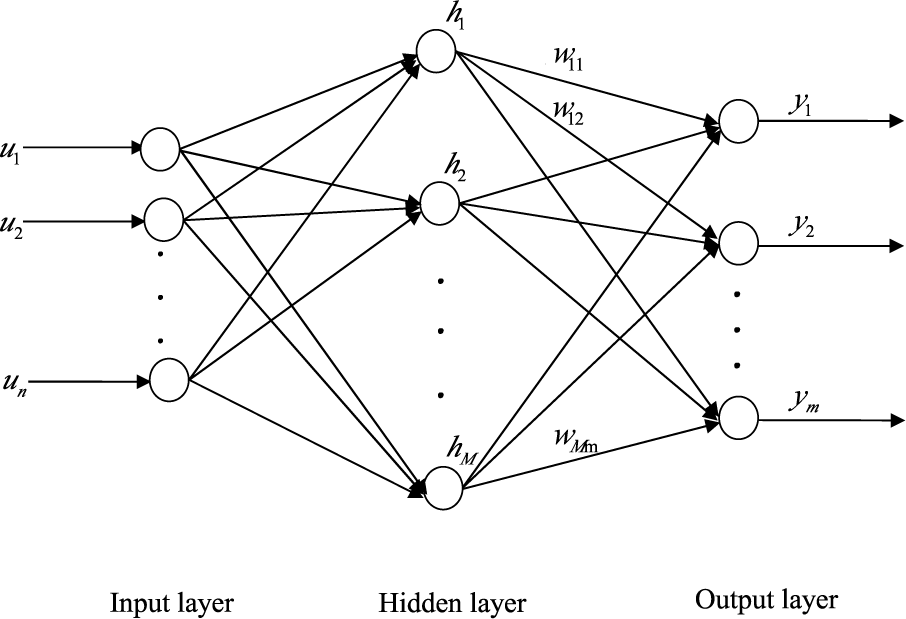
In these distributed ELM algorithms, the SLFN shown in
Figure 1 is used to learn the unknown nonlinear function at each node
k in the sensor network. We assume that the training data arrives one-by-one. Thus, at each time
i, given the input
uk,i for each node
k, the corresponding output of this node is:
where
hk,i = [
hk,i1,…,
hk,
im] is the output vector of the hidden layer with respect to the input
uk,i of node
k. For different RBF hidden neurons of the SLFN in one node, we use different centers and impact widths. For the SLFNs used at different nodes in the network, we use the same sets of centers and impact widths. In the following discussions, we first give the derivation of dELM-LMS algorithm. After that, we present the derivation of dELM-RLS algorithm. Notice that there are some differences between the derivation of the distributed ELM algorithms in this paper and that of the diffusion LMS and RLS algorithms in the literature [
1,
22,
23,
25,
26], so we present the derivation in detail.
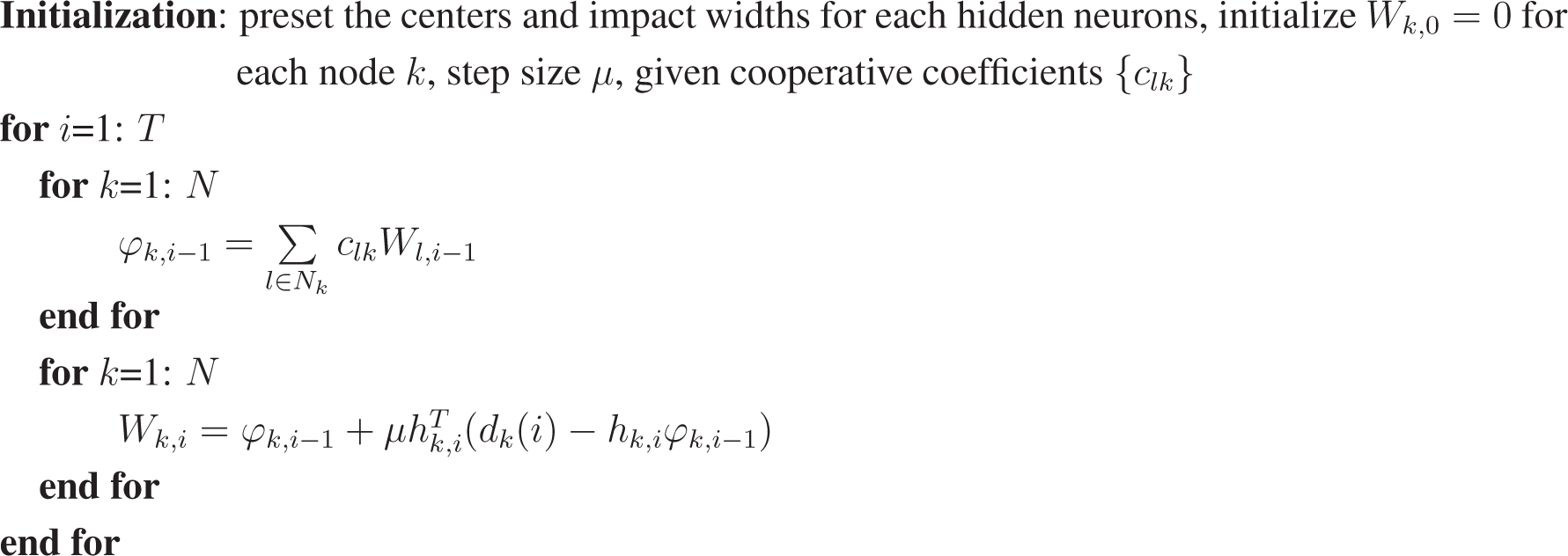
3.1. Distributed ELM-LMS
In the dELM-LMS algorithm, for each node
k in the sensor network, the local cost function is defined as a linear combination of local mean square error (MSE), that is:
where
W is the output weight matrix of the SLFN,
hl,i is the output vector of the hidden layer with respect to the input
ul,i of the node
l ∈
Nk and {
clk} are the non-negative cooperative coefficients satisfying
clk = 0 if
l ∉
Nk,
1TC =
1T and
C1 =
1. Here,
C is an
N ×
N matrix with individual entries {
clk}, and
1 is an
N × 1 vector whose entries are all unity. The cooperative coefficient
clk decides the amount of the information provided by the node
l ∈
Nk to node
k and stands for a certain cooperation rule. In distributed algorithms, we can use different cooperation rules, including the Metropolis rule [
28], the adaptive combination rule [
29,
30], the Laplacian matrix [
31] and the relative degree rule [
1]. In this paper, we use the Metropolis rule as the cooperation rule, which is expressed as:
where
nk and
nl are the degrees (numbers of links) of nodes
k and
l, respectively.
Given the local cost function for each node
k in the network, the steepest descent method is adopted here. The derivative of
(8) is:
Based on the steepest gradient descent method, at each time
i, for each node
k, we update the output weight matrix of the SLFN using:
where
Rl,h and
Rl,dh are the auto-covariance matrix of
h and the cross-covariance matrix of
h and
d at node
l, respectively,
Wk,i is the estimate of the output weight matrix of node
k at time
i and
μ is the step size. As we adopt the LMS type algorithm, namely an adaptive implementation, we can just replace these second-order moments by instantaneous approximations, that is:
By substituting
(12) into
(11), we obtain:
In order to compute
Wk,i defined in
(13), we need to transmit the original data {
dl(
i),
hl,i} of all nodes
l,l ∈
Nk to node
k at each time
i. We should notice that it brings a considerable communication burden to transmit the original data of all neighbor nodes of each node
k at each time
i. To tackle this issue, as in the diffusion learning literature [
1,
5], in this paper, we introduce an intermediate estimate. At time
i, we denote the intermediate estimate at each node
k by
φk,i. We then broadcast the intermediate estimate
φk,i to the neighbors of node
k. At time
i, for each node
k, the local estimate expressed by the intermediate estimates of its neighbors can be written as:
We now give some remarks on the rationality for doing so. First, the intermediate estimate contains the information of measurements. In addition, transmitting the measurements of neighboring nodes does not provide a significantly better performance. Thus, we do not need to transmit the measurements. Besides, we can update the intermediate estimate for each node k at each time instant, but do not transmit the intermediate estimate at each time instant, which will further significantly reduce the communication burden. Although we transmit the intermediate estimate at each time instant in this paper, the performance of the dELM-LMS algorithm transmitting the intermediate estimate periodically (with a short period) is quite similar.
Replacing the first
Wk,i–1 on the right-hand side of
(13) by
equation (14), we obtain:
Substituting
Equation (14) into
Equation (15), we can derive an iterative formula for the intermediate estimate, that is:
As
Wk,i-i is not available at node
l, l ∈
Nk \ {
k}, we cannot compute the value of the intermediate estimate of node
l by the above equation. Similar to [
5], we replace
Wk,i–1 in the above equation by
Wl,i–1, which is available at node
l. Thus, we obtain:
The simulation results demonstrate the effectiveness of this replacement. In addition, detailed statements about the rationality of this replacement are presented in [
5]. In this paper, we omit it for simplicity.
We replace the intermediate estimate
φl,i–1 in the above equation by
Wl,i–1, which is based on the following several facts. From
(14), we know that
Wl,i–1 is the linear combination of
φl,i–1; thus,
Wl,i–1 contains more information than
φl,i–1 [
1,
32], and it has already been demonstrated that such a replacement in the diffusion LMS can improve the learning performance. Moreover, the vectors
Wl,i–1 and
φl,i–1 are both available at the node
l. Based on this replacement and performing the “adaptation” step first, we acquire the two-step iterative update formula of the adapt-then-combine (ATC) type.
Alternatively, in each iteration, we can perform the “combination” step first, which leads to a combine-then-adapt (CTA)-type update formula. In the following, we sketch the derivation of this type of update formula.
From the discussion in the above, we know that
. In addition,
Wk,i–1 is independent of
. Thus, we can multiply the first
Wk,i–1 on the right-hand side of
(13) by
. Then, substituting
(14) into the left-hand side of
(13), we can get:
Based on the above equation, it is immediate to obtain another iterative formula for
φl,i, which is:
Similarly, we replace
Wk,i–1 in
(20) by
Wl,i–1, leading to:
The two-step iterative formula is:
From the above derivation, we know that Wk,i and φl,i are the intermediate estimate and the local estimate for node k at time i, respectively. In order to avoid causing notational confusion, we exchange the notations of W and φ. Consequently, we obtain the two-step CTA-type iterative formula.
For the purpose of clarity, the procedure of the ATC dELM-LMS algorithm and the CTA dELM-LMS algorithm are summarized in
Algorithm 1 and
Algorithm 2, respectively.
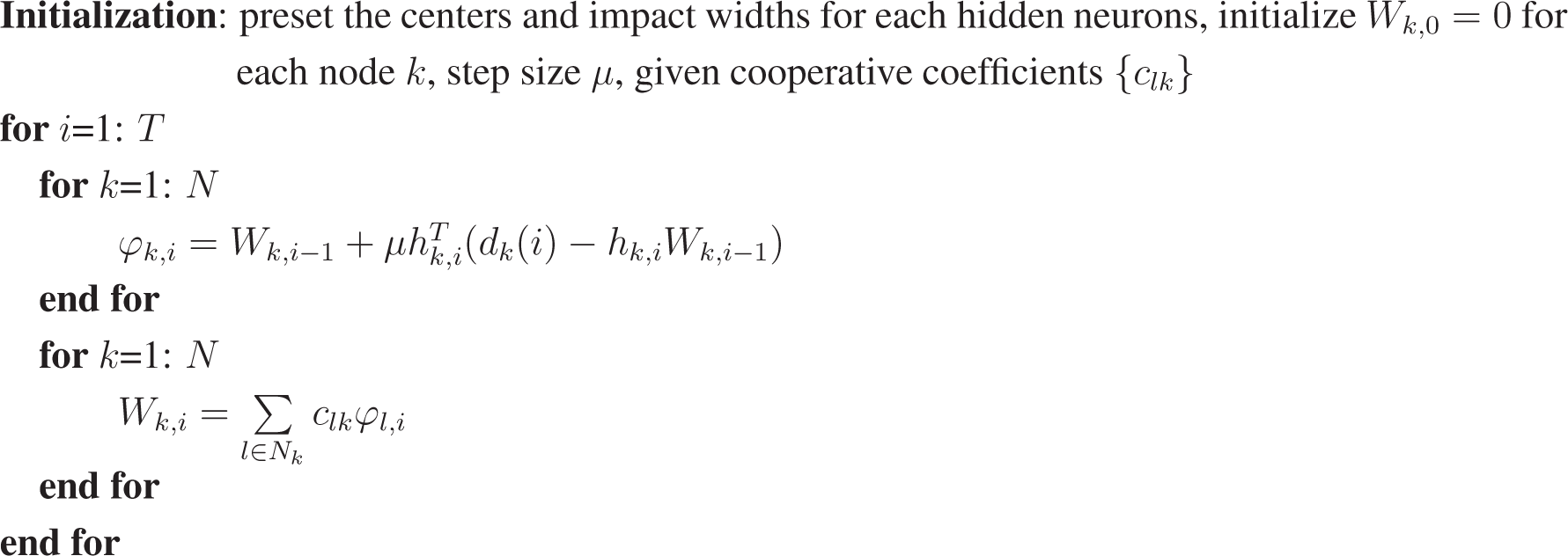
Algorithm 1:.
ATC dELM-LMS algorithm.
Algorithm 1:.
ATC dELM-LMS algorithm.
![Entropy 17 00818f8]() |
Algorithm 2:.
CTA dELM-LMS algorithm.
Algorithm 2:.
CTA dELM-LMS algorithm.
![Entropy 17 00818f9]() |
Remark 1. In the dELM-LMS algorithm, the local cost function of node k can also be defined as a linear combination of the modified local MSE [1],
where {
blk} are non-negative coefficients satisfying the conditions
blk = 0 if
l ∉
Nk and
, and
φl is the intermediate estimate available at node
l. After similar derivation as that performed in the dELM-LMS algorithms, we can obtain the more general two-step update equation. Performing the “adaptation” step first leads to another ATC-type iterative update formula.
Here, {
alk} are non-negative coefficients satisfying the conditions
alk = 0 if
l ∉
Nk and
. In a similar way, performing the “combination” step first leads to another CTA-type iterative update formula.
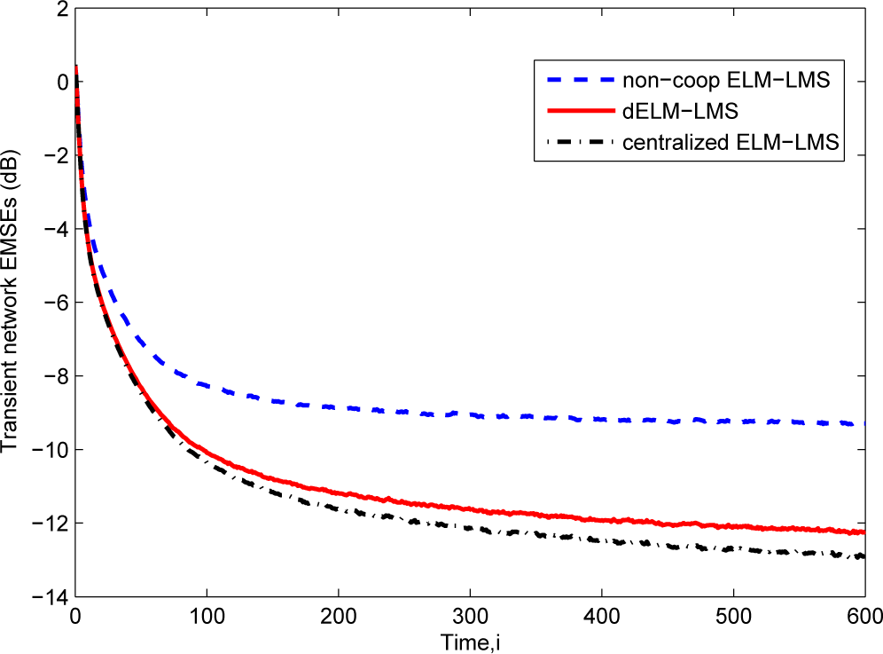
Notice that, using the above algorithms, in the case of C ≠ I, each node needs to broadcast the measurements to its neighboring nodes. As motioned in the above section, transmitting the data is a considerable communication burden. However, when the communication resources are sufficient, we can select transmitting the measurements. Through simulations, we find that transmitting the measurements does not provide significant additional advantages. Thus, in this paper, we omit the simulation results of these algorithms for simplicity.
3.2. Distributed ELM-RLS
In this dELM-RLS algorithm, at time
i, for each node
k, given the measurements collected from Time 1 up to Time
i, the local cost function is defined as:
where λ is the forgetting factor and Π
i is the regularization matrix. In the RLS algorithm, at each time
i, we use the forgetting factor λ to control the amount of the contribution of the previous samples, namely the samples from Time 1 up to Time
i–1. In addition, in this paper, we use the exponential regularization matrix
λiγ
−1I, where γ is a large positive number. We also use the Metropolis rule as the cooperation rule in this dELM-RLS scheme. The regularization item is independent of
clk, and
. Thus, we can rewrite
Equation (27) as:
Based on the above cost function, for each node
k, we can obtain the recursive update formula for the weight matrix by minimizing this local, weighted, regularized cost function, which can be mathematically expressed as:
Similar to the dELM-LMS algorithm, we also define and transmit the intermediate estimate of
Wk,i here. Then, replacing the
Wk,i in
Equation (29) by
Equation (14), we can obtain the following minimization of the intermediate estimate:
Equation (30) can be referred to as a least-squares problem. Based on the RLS algorithm, we can obtain the recursive update formula of the intermediate estimate for each node. Since the derivation of the recursive update formula of the intermediate estimate is the same as that presented in the centralized RLS algorithm, we omit the derivation for simplicity in this paper. Finally, we can obtain the two-step recursive update formula for the weight matrix. By performing the “adaptation” step first, we acquire the ATC dELM-RLS algorithm.
Similarly, we can also obtain the mathematical formula of the CTA dELM-RLS algorithm by just exchanging the order of the “adaptation” step and the “combination” step in each iteration.
In order to clearly present the whole process of the ATC dELM-RLS algorithm and CTA dELM-RLS algorithm, we summarize them in
Algorithm 3 and
Algorithm 4, respectively.
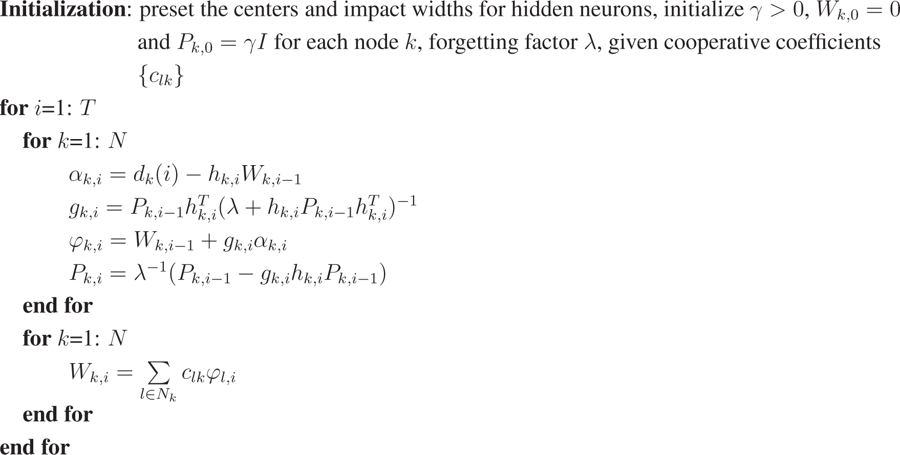
Algorithm 3:.
ATC dELM-RLS algorithm.
Algorithm 3:.
ATC dELM-RLS algorithm.
![Entropy 17 00818f10]() |
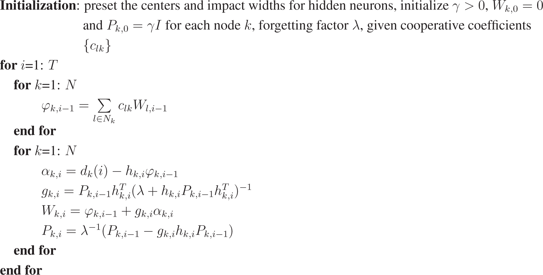
Algorithm 4:.
CTA dELM-RLS algorithm.
Algorithm 4:.
CTA dELM-RLS algorithm.
![Entropy 17 00818f11]() |
Based on the idea presented in [
26], we can also derive another ATC dELM-RLS algorithm and another CTA dELM-RLS algorithm, which exchange both the original data and the intermediate estimate among the neighbor nodes. Similar to the dELM-LMS case, in the simulation, we find that exchanging the original data does not provide a considerably better performance. Thus, for the purpose of simplicity, we omit the derivation and the simulation results of these dELM-RLS algorithms here.


