1. Introduction
Due to higher demands of power density for electric machines, investigations regarding the thermal management are getting more important. This ensures higher reliability and efficiency of the device, to name just two significant aspects. Inside an alternator, fan blades generate a pressure gradient by their rotational motion. Air from the engine bay streams through the alternator, flows through the rectifier domain and finally leaves the system in radial direction. In the rectifier domain, electronic components are pressed or glued on a heat sink. The design involves openings through the heat sink as well as ribs or pins. Therefore, the fluid undergoes different flow conditions that influence the heat transfer inside an alternator system. In most cases, a better cooling is in conflict with other aspects (e.g., costs or aeroacoustic emissions). A higher volumetric flow rate increases heat transfer, due to an increasing convective thermal energy transport. However, the maximum sound pressure level is strictly restricted as well and constrains the available range for the engineer. To detect local areas where heat transfer to the fluid could be intensified, a first obvious step is to check the temperature on the solid side. However, the temperatures show only the final outcome of the heat transfer. They convey no further information about the underlying processes. Looking only at temperatures, it cannot be found what is limiting heat transfer and where or why this occurs. Thévenin and Janiga [
1] showed how to combine Evolutionary Algorithms with Computational Fluid Dynamics (CFD) in order to optimize the flow for a wide range of engineering problems. Now, the analysis of entropy generation is a reliable approach to find regions with a high potential for such optimizations.
2. Entropy Generation Minimization
Bejan [
2] explained that “entropy generation through heat and fluid flows combines at the most fundamental level the basic principles of thermodynamics, heat transfer and fluid mechanics”. By investigating entropy generation information is obtained about the flow field and this gives the opportunity to find reasons for high local temperatures. It should be possible in this way to identify regions with a high potential for Optimization based on Computational Fluid Dynamics (written CFD-O), which will be used in this project [
1]. Based on this, design studies could be performed more efficiently, compared to a simple analysis of temperature fields.
2.1. Literature Survey
This chapter gives a short overview about previous studies of interest for the present investigations. Note that a complete overview about the entropy generation minimization (EGM) method can be found in, e.g., [
3] or [
4]. Poulikakos and Bejan [
5] derived the theoretical framework for an optimal fin geometry in forced convection using EGM. Fowler and Bejan [
6] obtained optimal sizes of bodies for external flows based on EGM. Wenterodt [
7] showed thanks to EGM that an optimal Reynolds number (Re) exists for a heated pipe. Carrington and Sun [
8] analyzed internal and external flows with the second-law analysis (SLA). Herwig and Schmandt [
9] used SLA to determine the drag coefficient for external flows with the help of the volumetric entropy generation in the flow field. Ko and Ting [
10] investigated the competition between the entropy generation due to dissipation and conduction for laminar forced convection in curved rectangular ducts with external heating. Şahin [
11] varied duct geometries, gave an analytical formulation and estimated the best geometry based on EGM. Mahmud
et al. [
12] presented an analytical solution for the entropy generation between two concentric rotating cylinders. Mirzazadeh
et al. [
13] extended the analytical solution for non-linear viscoelastic fluids. Yilbas [
14] computed temperature rise and entropy generation due to conduction and dissipation for this case. Further fundamental studies were done by, e.g., ([
15,
16,
17]). Giangaspero and Sciubba ([
18,
19]) used the entropy concept to study the thermal management for different electric machines. Many different authors ([
20,
21,
22,
23,
24]) used the EGM method to find an optimal heat-sink geometry. The present paper is a first step toward applying EGM for a real, industrial configuration. The first objective is to demonstrate the benefit obtained by analyzing the entropy budget compared to currently employed post-processing steps, for instance looking directly at the temperature fields.
2.2. Entropy Balance Equation
Following Bejan [
2], the total entropy generation
is the sum of entropy generation due to conduction
and entropy generation due to dissipation
:
where
and
are the time mean components and
and
are the fluctuation components for conduction and dissipation, respectively. After the temperature and velocity distributions of the flow field are solved, the time mean values can be calculated by the given temperature and velocity distributions from the solved flow field:
where
k is the thermal conductivity and
μ the dynamic viscosity. Equations (
2) and (
3) include the mean temperature and velocity gradients, respectively and represent the direct entropy generation in the mean flow field. However, if the flow becomes turbulent the terms resulting from the fluctuating parts of the flow field (involving
,
,
and
) are not directly available from any prediction based on RANS (Reynolds-Averaged Navier Stokes equations), and are difficult to measure directly with sufficient accuracy close to the wall, where it is most important:
Here,
in the denominator appears only in higher order terms when 1/T is expanded into a series and therefore is neglected in this leading order approach [
25]. To consider the fluctuation effects as well, Kock and Herwig ([
25,
26]) proposed a model with variables that are delivered by any commercial CFD-code:
where
β was found to be
β = 0.09. With Equations (
6) and (
7) the fluctuation terms from Equations (
4) and (
5) can be modeled when using, e.g., Menter’s
k-
ω-SST turbulence model. For other turbulence models, corresponding formula can be found in, e.g., Kock [
27]. Finally, the total entropy generation for turbulent flows becomes a post-processed value computed by a volume integral of the local values over the domain of interest:
3. Canonical Configuration
A three-dimensional numerical study of an electric alternator delivers a huge quantity of data. Due to the geometrical and physical complexity of the setup a large number of finite volumes have to be used for a simulation (small cells being especially needed in near-wall regions). In most cases, a detailed quantitative analysis of these data is not performed. Therefore, further investigations regarding new physical indicators like, e.g., entropy generation are necessary to support, facilitate and speed-up the analysis. To enable the development of such indicators, a simplified but relevant configuration has been first identified, called “canonical configuration” in this work. Eger
et al. [
28] introduced the concepts underlying this configuration and showed its benefit based on a Nusselt number analysis.
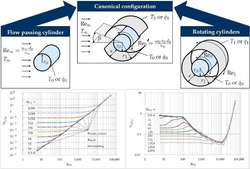
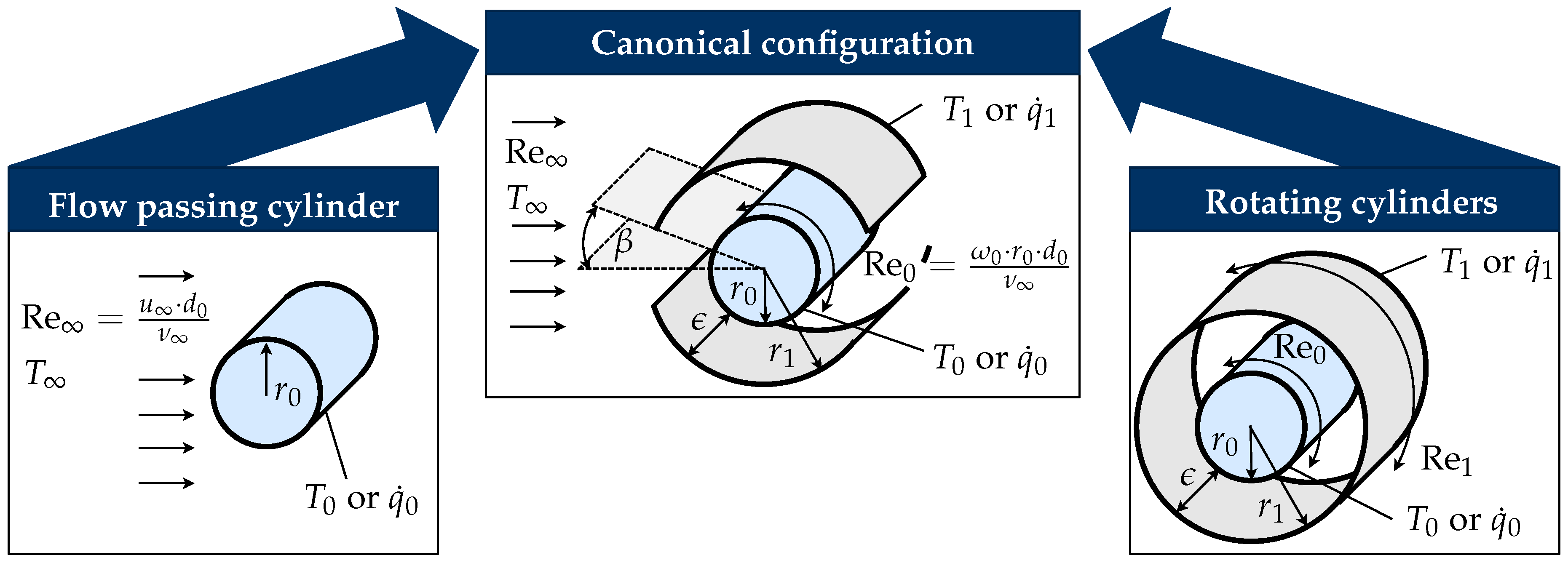
Figure 1 explains the choice of the canonical configuration. Using it, it is possible to investigate fluid processes and heat transfer at different scales, controlled either by ambient parameters (global scale “
∞”) or by near-wall gradients (local scale “
”), alone or in combination, while keeping a single geometrical setup described by a small number of parameters. Thanks to such a simple configuration, the quantity of data that must be analyzed is heavily reduced. However, the transport phenomena found in real electric alternator systems are still represented.
Figure 1.
Canonical configuration used for further investigations of transport phenomena and for the development of physically-based indicators of heat transfer.
Figure 1.
Canonical configuration used for further investigations of transport phenomena and for the development of physically-based indicators of heat transfer.
Thus, the canonical configuration offers the opportunity to investigate physically-based indicators, e.g., entropy generation, with a high level of generality. Ultimately, a thermal optimization of electric machines regarding fluid and heat transport should become possible. The opening angle
β in main flow direction defines the openings on both sides. Its range is obviously defined by
. The gap
ϵ between the rotating cylinder and the external sleeve is strictly positive. Compared to a single cylinder, two additional design parameters have been added, here
β and
ϵ.
Table 1 gives an overview about the parameters that have an influence on the flow field locally (within the annuli) as well as globally (in the whole domain).
Table 1.
Parameters influencing the flow and temperature field.
Table 1.
Parameters influencing the flow and temperature field.
| | Locally | Globally |
|---|
| Dynamic | | |
| Heat transfer | | |
| Design | | β |
The ratio of outer () and inner radius () is defined as Π. The tangential velocity of the rotating cylinder is defined with , where is the angular velocity of the rotating cylinder. The oncoming flow at the channel inlet is expressed by . For an increasing opening angle , the canonical configuration converges toward the (external) flow around a cylinder. A decreasing opening angle leads to the study of the (internal) flow between two concentric rotating cylinders. For the range transport processes involve both aspects.
4. Physical Model
The problem described in the previous section can be considered either as a three-dimensional or a two-dimensional problem.
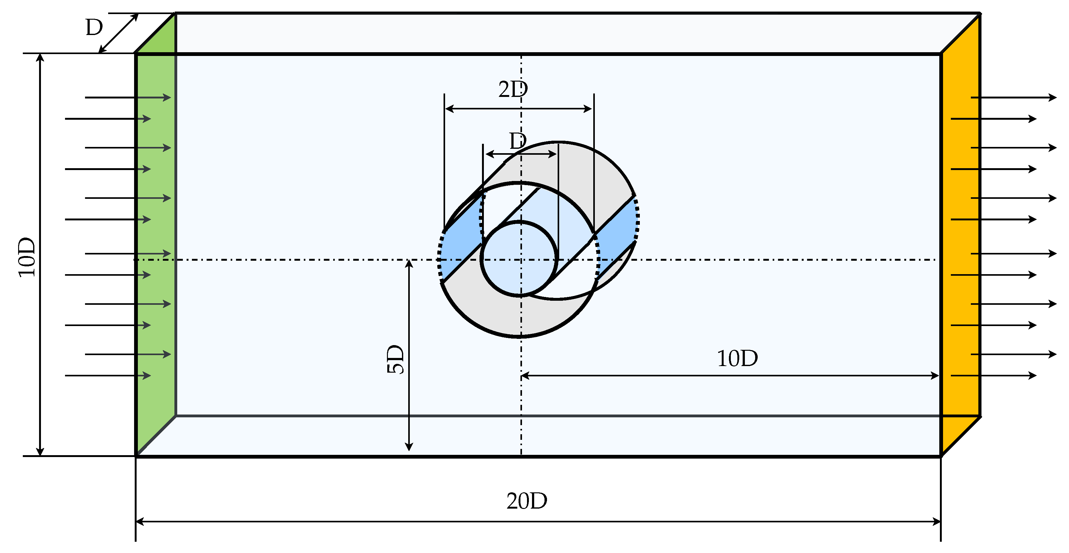
Figure 2 shows the cylinder and sleeve mounted in a rectangular domain, constructed as a three-dimensional problem with symmetry boundary conditions in cross direction.
Figure 2.
Dimensions of the first geometrical setup based on the canonical configuration.
Figure 2.
Dimensions of the first geometrical setup based on the canonical configuration.
As further boundary conditions, velocity inlet (left side of the domain) and pressure outlet (right side of the domain) are systematically employed for all computations. In these investigations, two different Reynolds numbers are important, written
and
(see
Figure 1):
For practical purposes, the focus is set on the transport phenomena between the cylinder and surrounding sleeve. Therefore, the channel can be constructed without an increased wake region to reduce the numerical effort. The sleeve is defined as adiabatic and the wall of the rotating cylinder with an isoflux boundary condition. The heat flux is expressed in dimensionless form
which is defined as:
The ambient temperature is constant with a value of K. The flow field in all following simulations is considered as steady and incompressible. Ideal gas has been chosen as working fluid (air in this study). Due to the small temperature change in the flow field, the thermo-physical properties such as dynamic viscosity μ and thermal conductivity k are assumed constant with values of and , respectively. Using the canonical configuration for a first study, the design parameters were set to and . In this case the transport processes involve external and internal flows and therefore describe the processes found in a real alternator system. The ratio between the outer and inner tangential velocity is defined as , due to the static sleeve around the cylinder. However, the inner cylinder is in rotation, which is expressed by . Both Reynolds numbers ( for global changes of and for local changes of ) are varied in magnitude. The ranges for all simulations are and , changing the values by a factor 2 between two cases.
5. Numerical Method
The equations of conservation of mass, momentum, and energy are discretized with
ANSYS CFX 16.2, relying on the Reynolds-Averaged Navier Stokes (RANS) approach. In our investigations Menter’s
k-
ω-SST model is chosen due to its ability to integrate the Navier-Stokes equations in the low Re regime near the wall without using damping corrections. Additionally, it leads to better predictions of flow separation [
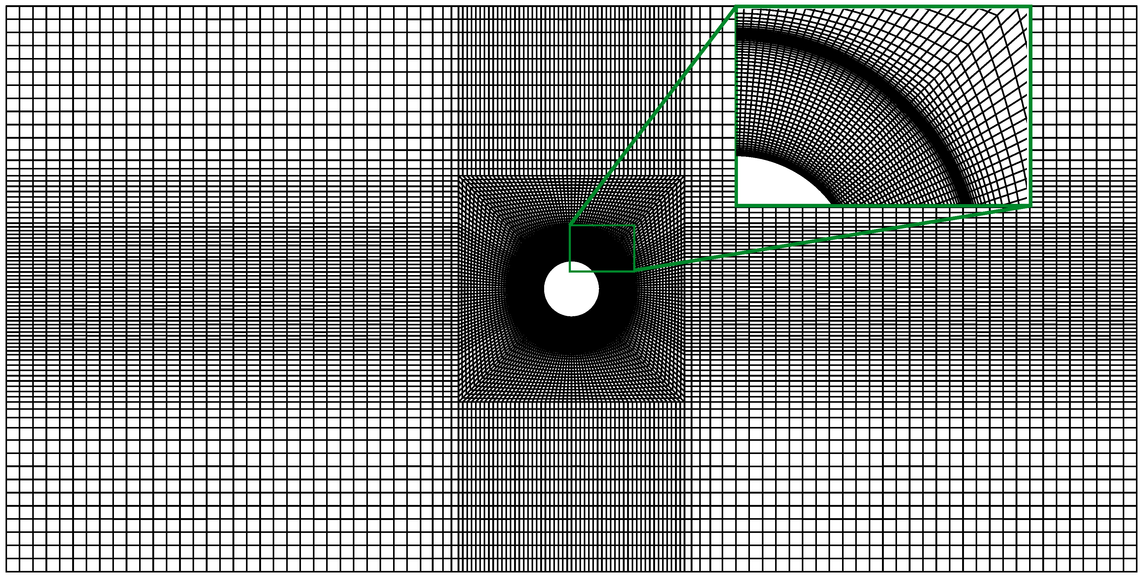
29]. The selected advection scheme uses a second-order scheme when possible and blends to a first-order scheme if needed to maintain boundedness. The flow equations are solved sequentially with double precision. For the grid, hexahedra elements are chosen, which are shown in
Figure 3, placing the first grid element at a dimensionless wall distance
, as needed for high accuracy [
30]. This results in very small elements near the walls of the cylinder and the sleeve, due to high velocity gradients.
Figure 3.
Hexahedral grid employed for the canonical configuration.
Figure 3.
Hexahedral grid employed for the canonical configuration.
Starting with an element size of
mm and a growing ratio of
, the total number of elements is about 272,700. The convergence criteria for momentum and mass, heat transfer, turbulence and the additional terms of
are set as a factor of
. To check the convergence behavior of the entropy generation terms, Equation (
8) was completely implemented within the solver. For this purpose, additional variables were defined into the model settings, allowing a direct computation of entropy generation after each iteration solving the conservation equations for mass, momentum and energy. Therefore, entropy generation is directly calculated within the solver and can be immediately analyzed. Due to the high values of
and
included in the range of interest, viscous dissipation has to be considered within the energy equation in principle. Note that no difficulties have been encountered concerning convergence when including the viscous work term.
6. Grid-Independence Test and Code Verification
Grid-independence tests and code verification were carried out for the two cases shown in
Figure 1.
6.1. Internal Flow: Two Concentric Rotating Cylinders
First, the flow between two concentric rotating cylinders has been investigated as an example for an internal flow (corresponding to the local flow between the two cylinders for the canonical configuration at
). The physical and numerical models described above are used for both examples. Following Yilbas [
14], the flow in the annuli is laminar since
is below the critical value:
The dimensionless temperature difference between the outer and inner cylinder is defined as:
(assuming that
). The dimensionless radial distance is
. The Brinkman number (Br) is the ratio between the thermal energy that is produced due to dissipation and the ability of the fluid to evacuate this energy:
In order to obtain a suitable Br value, and only for this case, the dynamic viscosity
μ was artificially changed to
.
Figure 4 shows the numerically calculated dimensionless entropy generation profiles (
) compared to the analytical solutions from Mirzazadeh [
13] for a varying ratio
. The dimensionless entropy generation terms are calculated as:
for isoflux (
) or isothermal (
) boundary condition, respectively.
Figure 4.
Effect of on for , and (isothermal boundary condition).
Figure 4.
Effect of on for , and (isothermal boundary condition).
The numerical solutions are systematically in excellent agreement with the analytical solutions for the cases with
, when Br is constant and Ω is changed in magnitude. In
Figure 4, both cylinders are associated with an isothermal boundary condition.
6.2. External Flow: Flow Passing Cylinder
In a further study, the flow passing an infinite cylinder has been investigated as an example of pure external flow (corresponding to the global flow for the canonical configuration at
). The Reynolds number
(defined with the oncoming flow
) is varied in magnitude in a range of
, which is large enough to cover all following investigations, leading to a maximum of
. For a detailed grid-independence test and code verification, the integral values of
and
in the complete domain around the cylinder are considered. Therefore, an increased size of the channel is needed to capture all entropy generation terms in the wake region. In this case, the wake region is extended to a size of twenty-two times the cylinder diameter. The other geometrical parameters are kept constant as it is shown in
Figure 2. Following Bejan [
31], the entropy generation terms on an immersed body can be calculated as:
where
is the drag force:
The comparison to the numerical solutions are shown in
Figure 5. Experimental values of the drag coefficient (
) for the flow passing a cylinder are available in many textbooks, e.g., Zierep [
32].
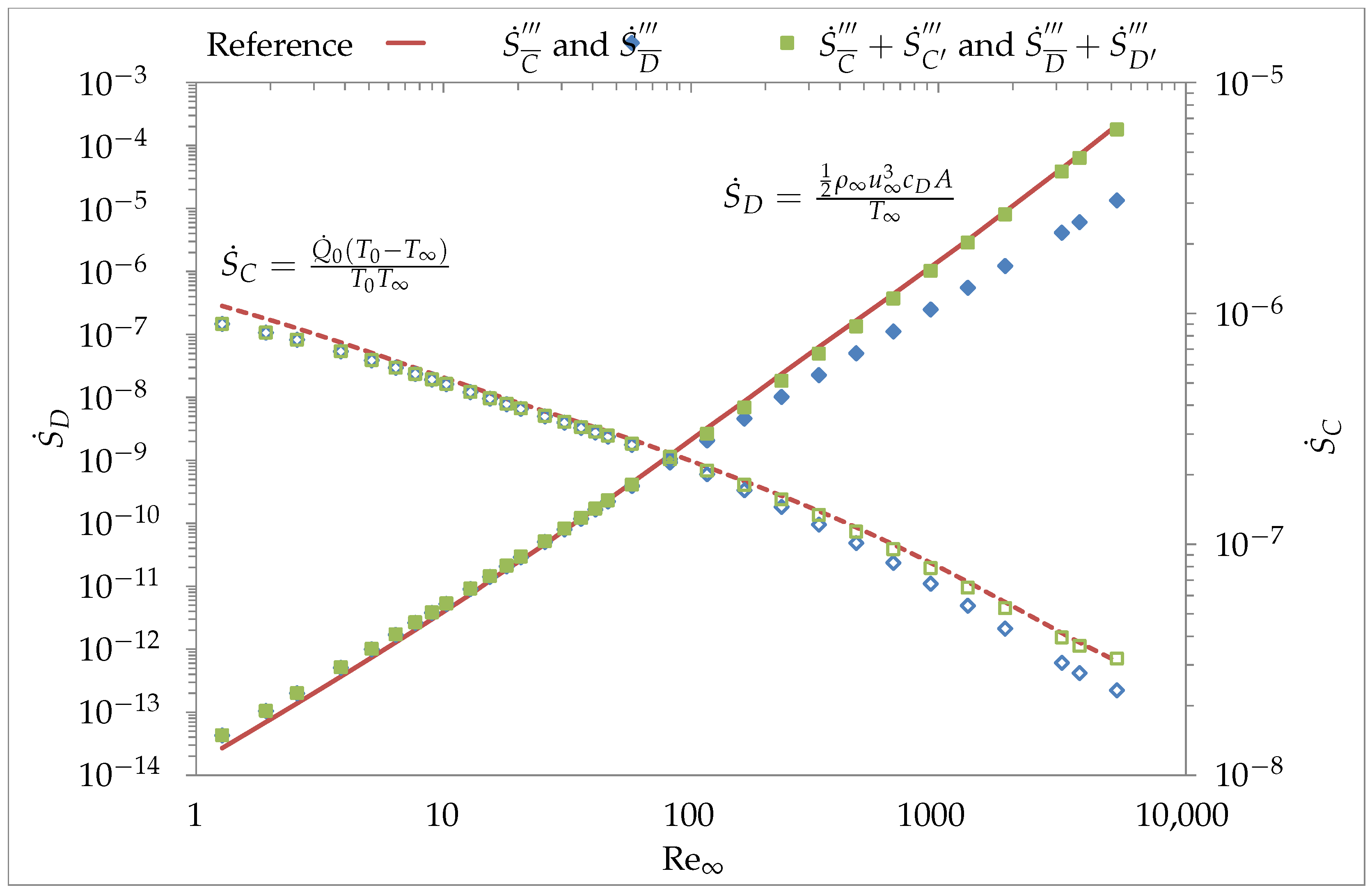
Figure 5.
Comparison between reference obtained analytically (with Equation (
13)) and experimentally (with
for varying
) with numerical results obtained for
and
. The symbols correspond to the numerical results of the present study with only the mean components (blue) or accounting additionally for fluctuation components (green). Solid line and filled symbols are for
, dashed line and hollow symbols for
.
By substituting the experimental results in Equation (
14) for different
values, the entropy generation due to dissipation
can be calculated. Therefore, the analytical calculation of
becomes possible with experimental data of
. The entropy generation due to conduction
can be calculated with the given thermal boundary condition. In the current case, an isoflux boundary condition (
) is used to calculate numerically the resulting wall temperature
. The mean components (
and
) show steadily increasing discrepancies for
. However, including the fluctuation components (Equations (
6) and (
7)) in the entropy generation equation, the values are in a very good agreement with the reference for the whole range considered for
.
This concludes the successful verification of the developed numerical approach. For the tested configuration of the flow between two concentric rotating cylinders, the numerical results are identical or very close to the analytical predictions. For the flow passing a cylinder the analytical observations combined with experimental data for showed a very good agreement to the numerical solutions as well. However, a grid wall resolution is as expected needed for an accurate analysis of flow, heat transfer, and associated entropy generation.
7. Results And Discussions
Using now the canonical configuration for a first full-scale study, the design parameters were set as described in
Section 4. All diagrams show the results in a double logarithmic reference frame, except for the results of the dimensionless temperature difference
shown in
Figure 9. In
Section 7.1,
Section 7.2,
Section 7.3 and
Section 7.4 the integral (global) analysis of the entropy generation will be discussed.
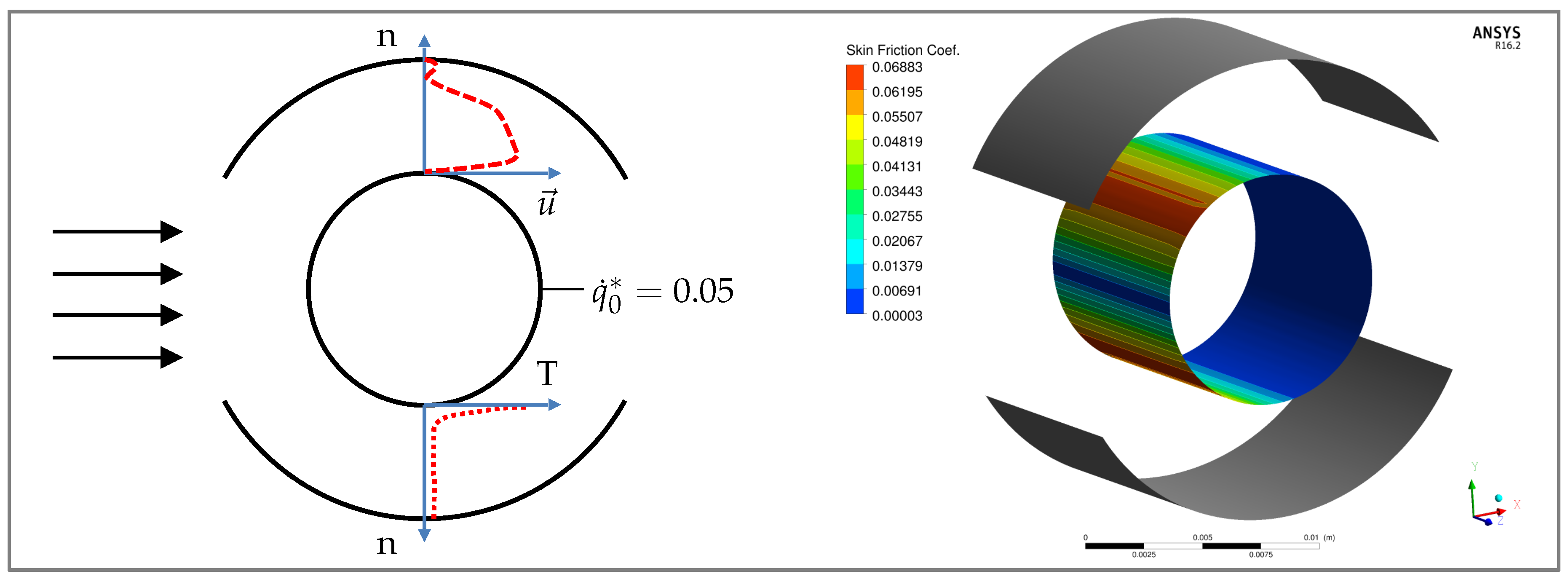
Section 7.5 gives an outlook about the possibilities offered by a differential (local) analysis. To allow a better understanding of the flow system,
Figure 6 shows in the left picture the flow velocity and temperature profiles. In the right picture, the skin friction coefficient
on the cylinder wall is shown.
Figure 6.
Left: Flow velocity (dashed) and temperature (dotted) profiles. Right: Skin friction coefficient on the cylinder wall for and , respectively.
Figure 6.
Left: Flow velocity (dashed) and temperature (dotted) profiles. Right: Skin friction coefficient on the cylinder wall for and , respectively.
7.1. Entropy Generation Due to Dissipation
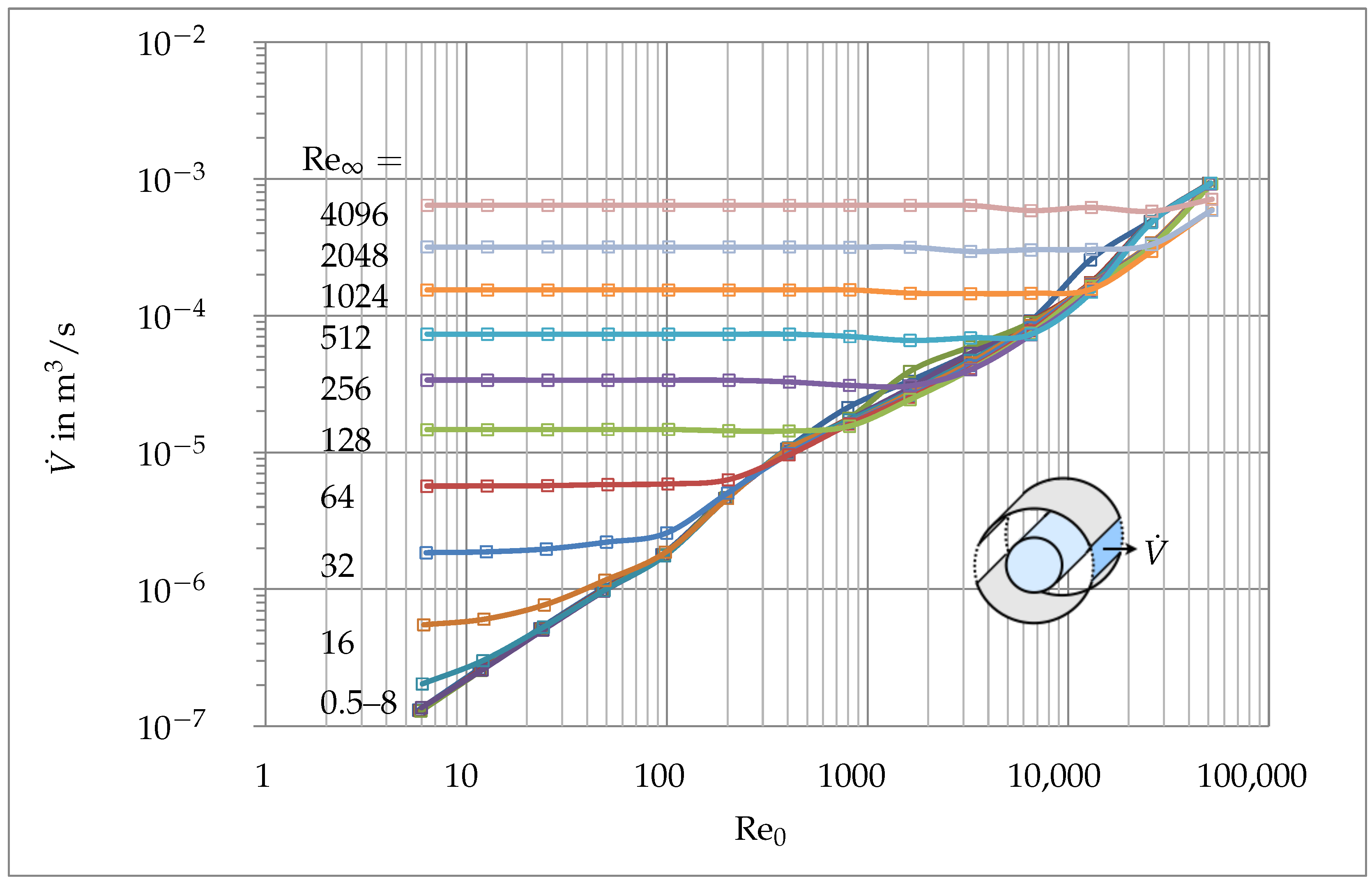
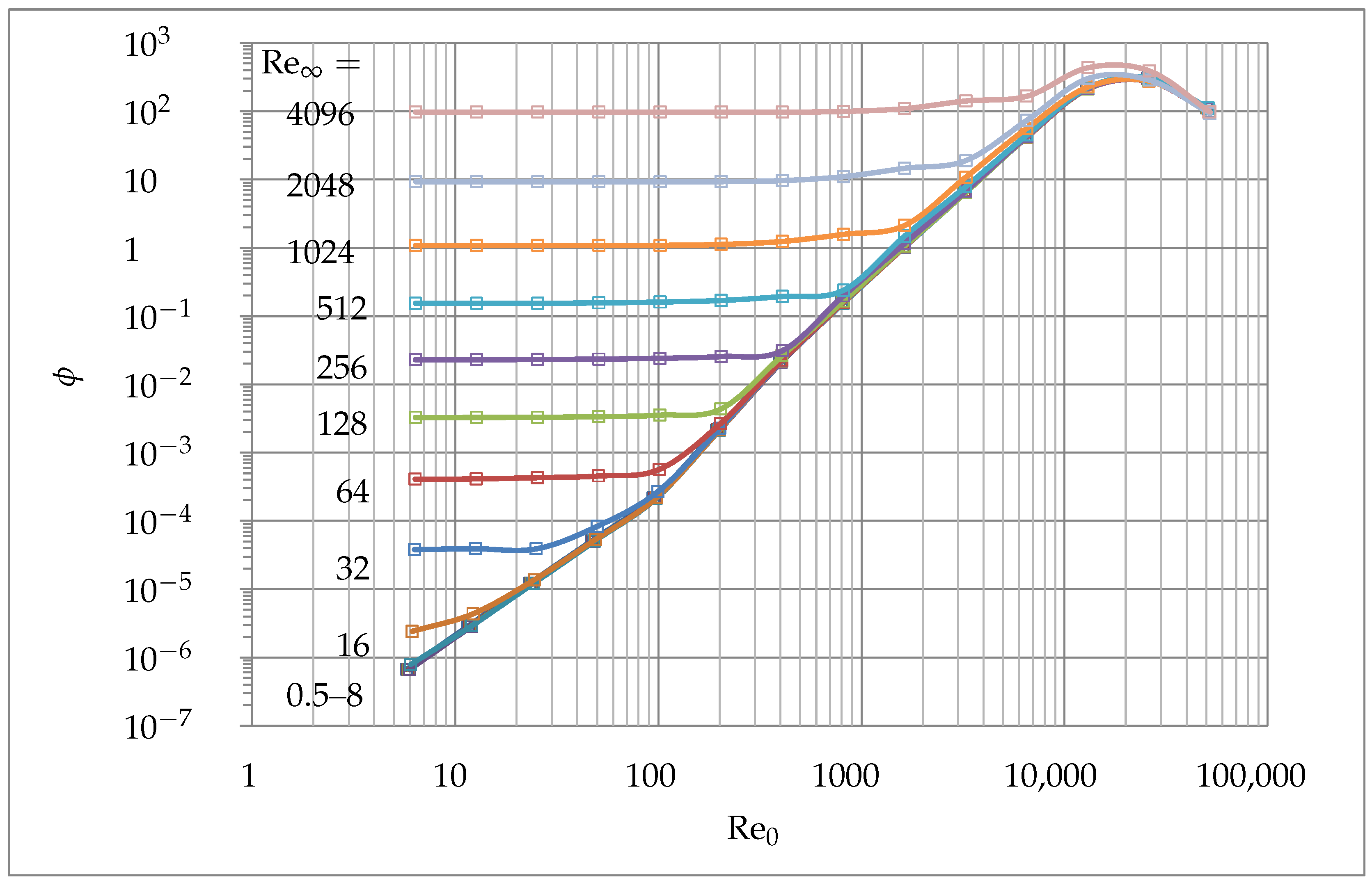
Figure 7 represents the very considerable change of the volumetric flow rate (
) obtained when varying Reynolds numbers (
and
). This quantity is computed on the interface located at the farther end of the sleeve, where the flow is leaving the annuli, as shown in
Figure 7.
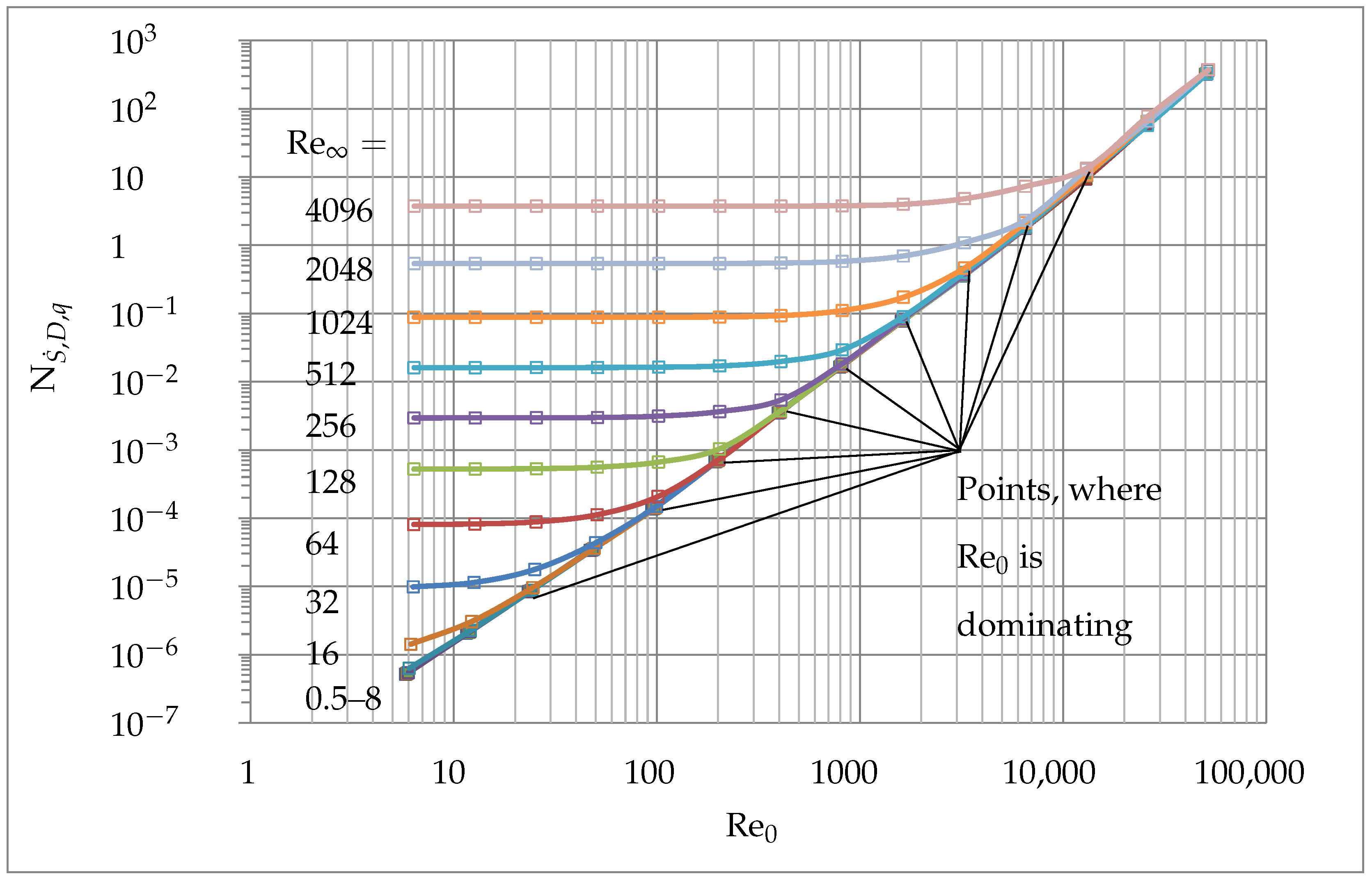
Figure 8 shows the same analysis with respect to the dimensionless volumetric entropy generation due to dissipation (
) between the rotating cylinder and static sleeve. Both results are in very good agreement and show similar trends. However
provides a smoother evolution. With an increasing Reynolds number (
or
) the volumetric flow rate and the dimensionless entropy generation due to dissipation increase as well. Hence, a reduction of the entropy generation due to dissipation is as expected directly connected to a reduction in flow speed and thus Reynolds number. For the range
the flow is always strongly influenced by the local tangential velocity
(
). The oncoming flow is too slow and has therefore no influence on the entropy generation due to dissipation. If, however, the magnitude of the global velocity
(quantified by
) increases, a higher local tangential velocity
(
) is needed to influence the flow field through the motion of the cylinder. The point where
is becoming the dominating effect is clearly identifiable for all
.
Figure 7.
Effect of and on .
Figure 7.
Effect of and on .
With , even the highest oncoming flow () has no real influence on the volumetric flow rate or on the entropy generation due to dissipation. As a consequence, the maximum of entropy generation due to dissipation is for all Reynolds numbers considered in this study. Such results demonstrate that the interaction between global ambient parameters (through ) and near-wall gradients (through ) is very important for the characterization of the flow field.
Figure 8.
Effect of and on .
Figure 8.
Effect of and on .
The expected positive effect caused by an increasing oncoming flow has under some circumstances no influence on the cooling, when dominates the process. In other words, an increasing volumetric flow rate in an alternator system can be without any effect if the flow field is mainly influenced by the ribs or openings in the rectifier domain, at local scale. Analyzing the entropy generation due to dissipation reveals such effects in a conspicuous manner.
7.2. Entropy Generation Due To Conduction
Figure 9 summarizes the results for the dimensionless temperature difference between the rotating cylinder and the ambient temperature
(assuming
), defined as:
Figure 9.
Effect of and on .
Figure 9.
Effect of and on .
For
the magnitudes considered are nearly identical to each other for
. For such conditions, the dimensionless temperature difference decreases slightly when increasing local Reynolds number,
. However, for cases with
the magnitude of
first increases till a specific value of
, and decreases later when increasing further
. All minima of the dimensionless temperature difference are around
for
. Varying
, the magnitudes of
are different from each other, the lowest temperature being found for the highest incoming flow,
. For the highest local tangential velocity (
) the obtained magnitudes also differ from each other.
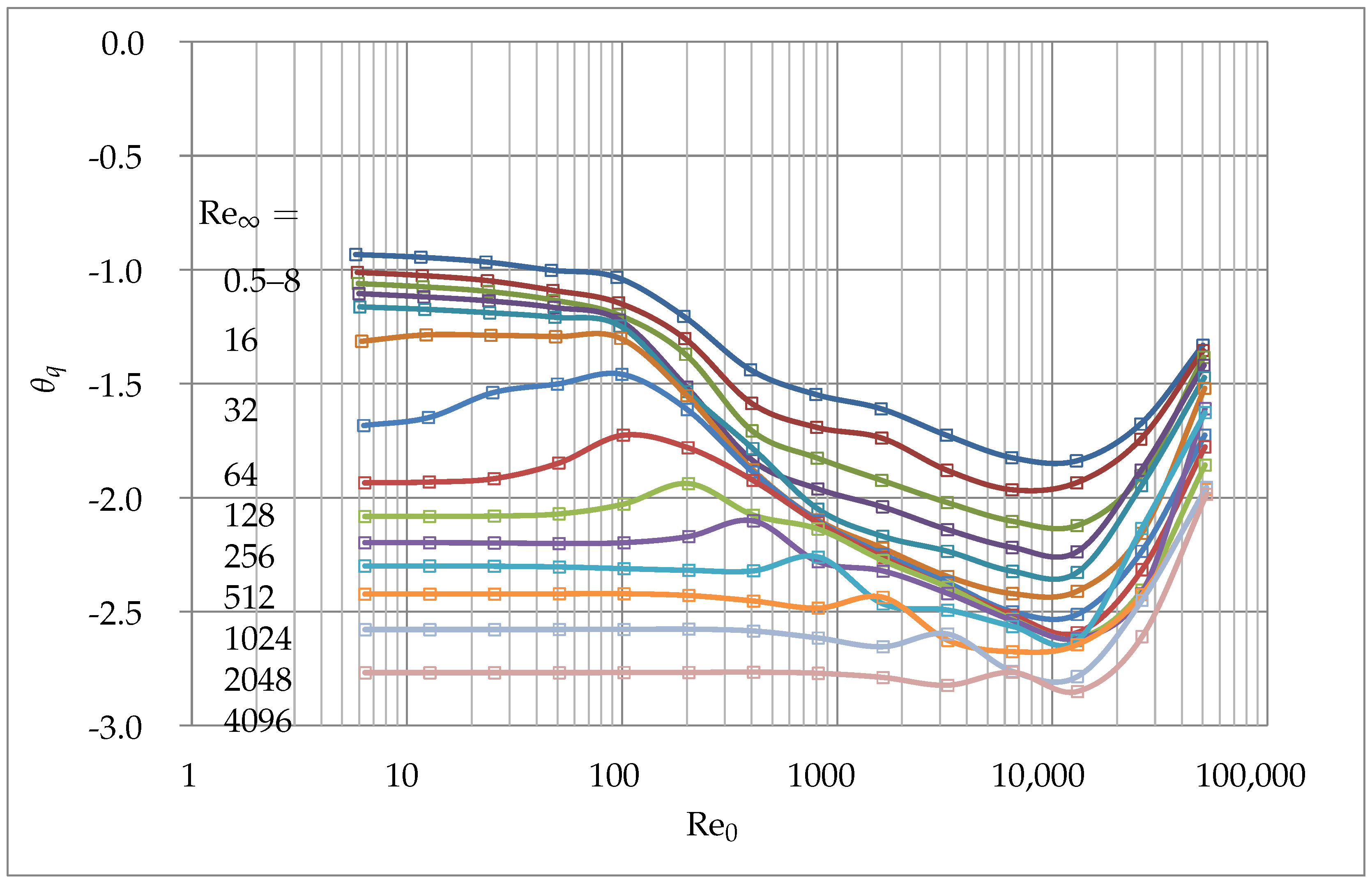
Figure 10 shows the results for the entropy generation due to dissipation
. In the range
the magnitudes of
are similar to each other and thus appear close to a single line. At low values of
, the magnitudes of
and
decrease monotonically with an increasing oncoming flow velocity (quantified by
). At
both variables (
and
) reach their lowest value. Therefore, it appears that the heat transfer increases with a higher global Reynolds number
, as expected. Regarding now
, the dimensionless temperature difference as well as the dimensionless entropy generation due to conduction reach their minima almost at the same position, independently of
in the range
:
Figure 10.
Effect of and on .
Figure 10.
Effect of and on .
Therefore, the dimensionless entropy generation due to conduction delivers the same minima as the dimensionless temperature difference for the cases considered. However, the dimensionless entropy generation shows a smoother course and a more marked minimum for conduction. Here, the minima is
for all
. For
the viscous dissipation becomes significant, leading to an increase in
as well as
. At
the entropy generation due to conduction reaches
for all
. For the range
the dimensionless temperature difference and the dimensionless entropy generation due to conduction show a local peak before the function reaches its global minima.
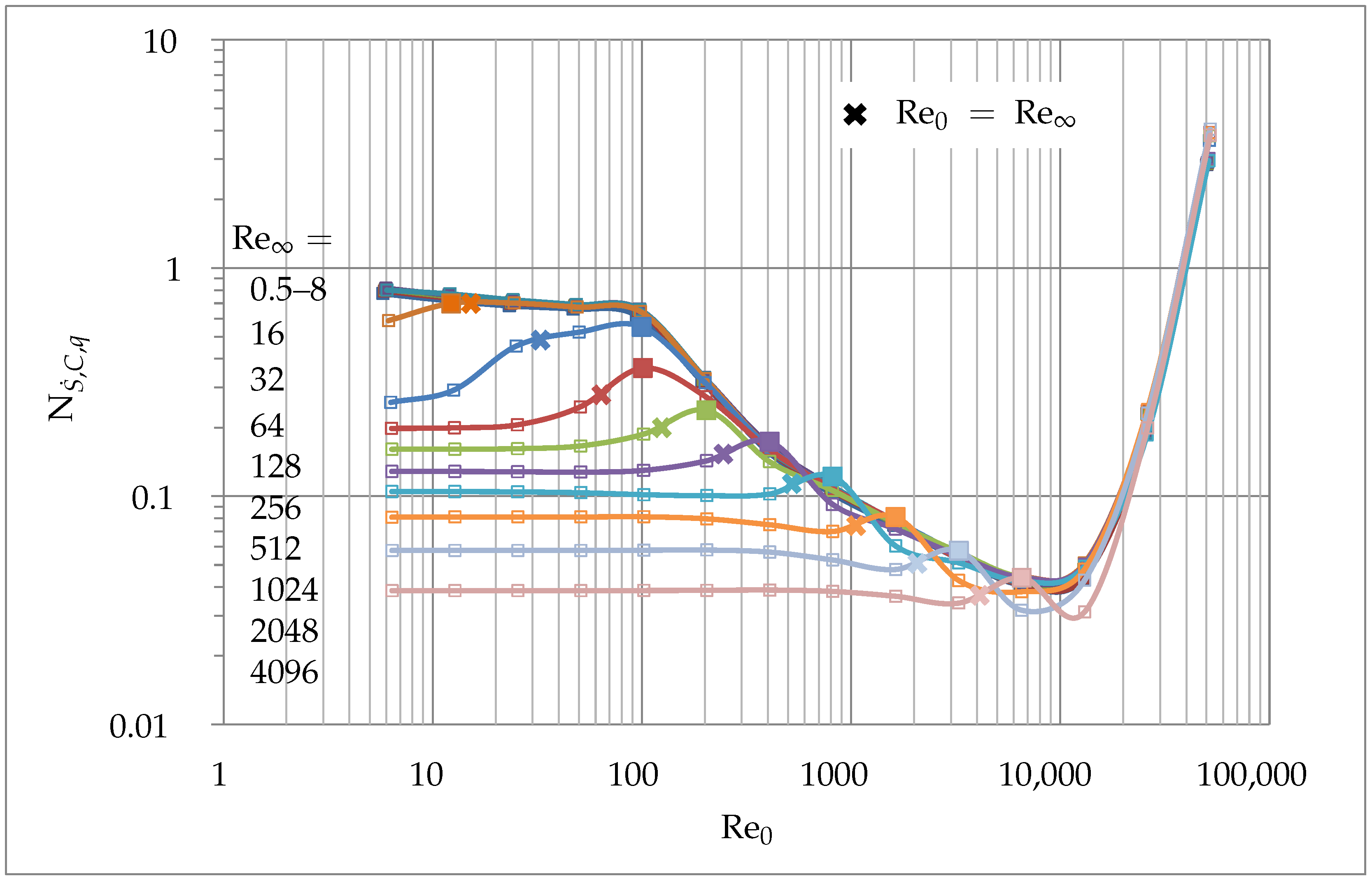
Figure 11 shows the local peak values as filled square symbols of the corresponding color. The points corresponding to the condition
are additionally shown as crosses. It can be observed that the local maxima are found shortly after the condition
. An explanation could not be found up to now.
As a whole, entropy generation due to dissipation shows results similar to the volumetric flow rate along the outlet interface. Entropy generation due to conduction delivers the same minima as the dimensionless temperature difference between the cylinder and the fluid. However, the entropy generation due to dissipation and to conduction have the same unit () and can thus be analyzed together. This simplifies the physically-based comparison between the two possibly concurrent objectives, minimizing and minimizing . The alternative comparison between () and (−) would be far more difficult to interpret.
Figure 11.
Points where is reached.
Figure 11.
Points where is reached.
7.3. Total Entropy Generation
From the previous
Section 7.1 and
Section 7.2 the following conclusions can be derived:
A lower entropy generation due to dissipation is associated to lower values of as well as .
A lower entropy generation due to conduction is correlated with an increasing .
The minima of entropy generation due to conduction are all observed close a specific value of (around ) for all .
Below this value, the flow field is too slow for an optimal convective thermal energy transport.
Above this value, fluid dissipation increases and therefore the temperature difference between fluid and solid gets smaller.
The final challenge is to find the best compromise between entropy generation due to dissipation and entropy generation due to conduction. A qualitatively similar competition was discussed in the introduction, discussing the competing goals between cooling and noise emissions.
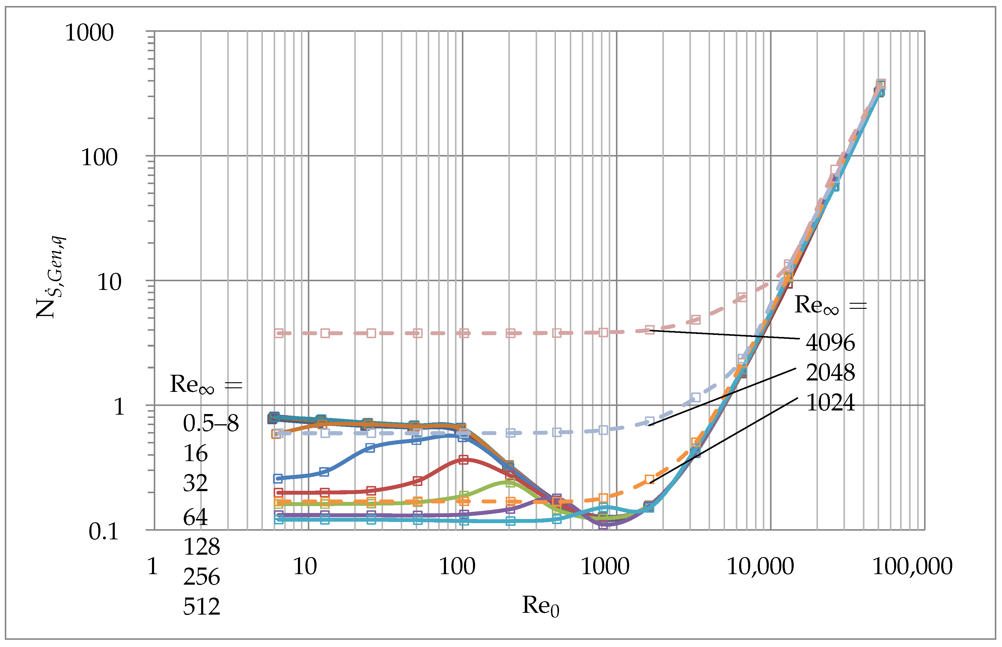
Figure 12 shows the sum of entropy generation due to dissipation and conduction (
). As it can be seen, the minima of
is at
, for all
.
This value is much smaller than the minima for the entropy generation due to conduction, which is at
. For
the total entropy generation is strongly influenced by the entropy generation due to dissipation and therefore follows the behavior of
, already shown in
Figure 8. The solid blue line corresponding to
in
Figure 12 shows the transition between both typical behaviors.
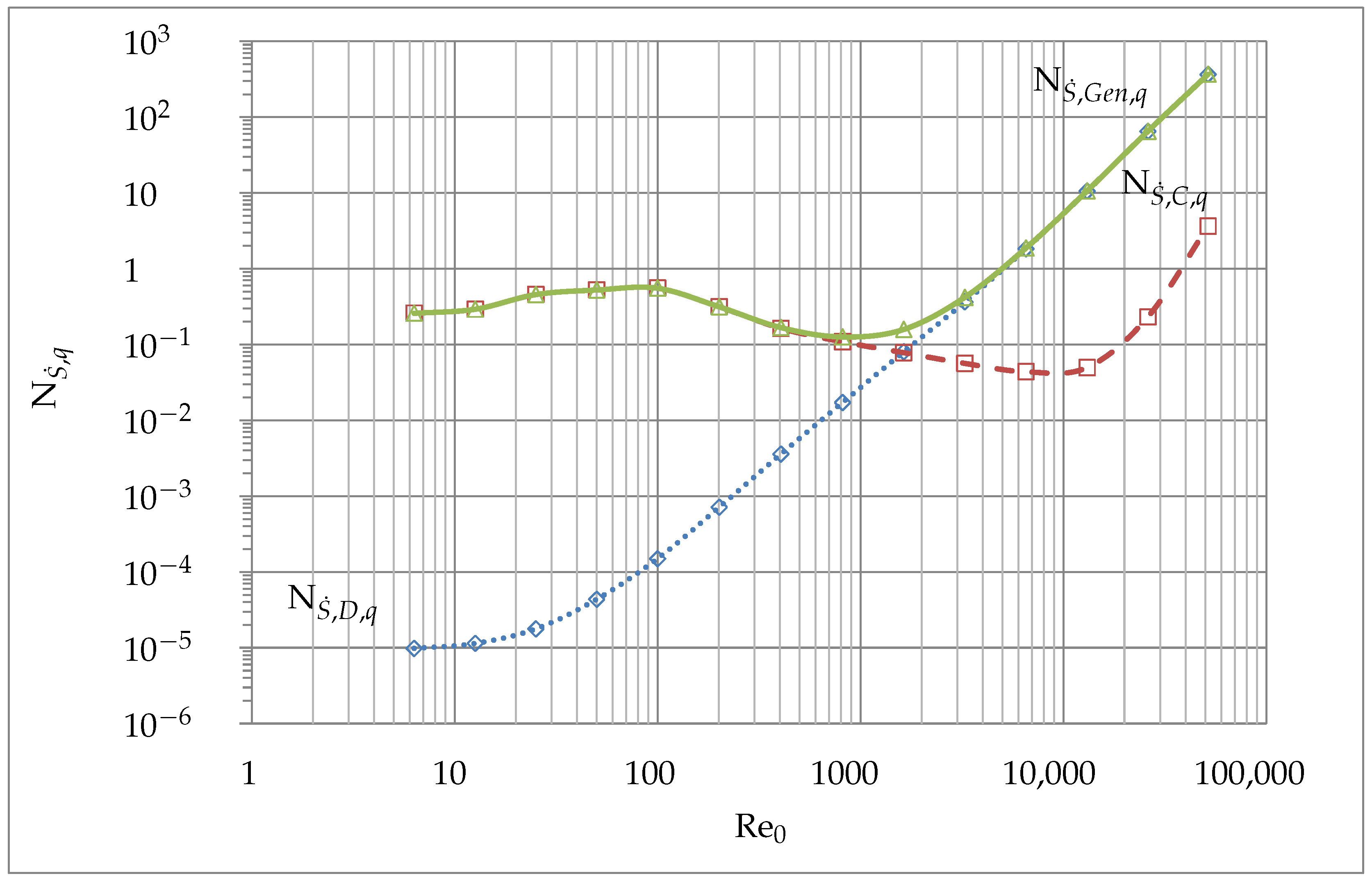
Figure 13 and
Figure 14 show
,
and
for
and
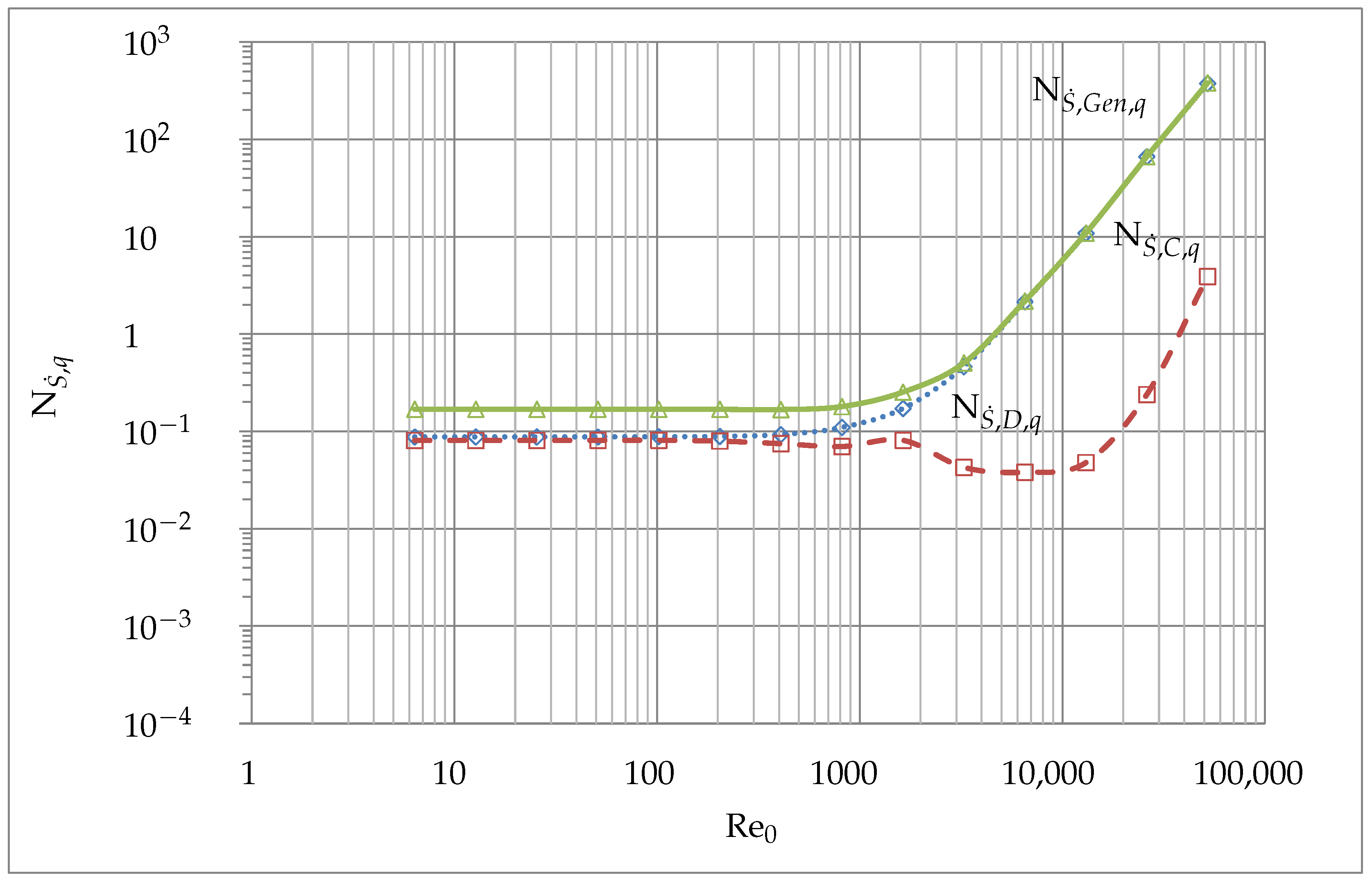
, respectively, these values being chosen as being representative of these two different regimes. For the case
in
Figure 13, the entropy generation due to conduction
is the dominating effect, till
. At this point the entropy generation due to dissipation
reaches the same magnitude and continues to grow with an increasing
. At
the total entropy generation
depends on the entropy generation due to dissipation, only. For the case
in
Figure 14,
and
have roughly the same magnitude, till
.
Figure 12.
Effect of and on .
Figure 12.
Effect of and on .
Figure 13.
(dotted, ◊), (dashed, □) and (solid, ∆) for .
Figure 13.
(dotted, ◊), (dashed, □) and (solid, ∆) for .
Figure 14.
(dotted, ◊), (dashed, □) and (solid, ∆) for .
Figure 14.
(dotted, ◊), (dashed, □) and (solid, ∆) for .
Hence, both have an influence on the total entropy generation . After this point the entropy generation due to dissipation becomes the dominating effect due to a higher and completely controls the total entropy generation above . The total entropy generation shows an earlier minimum as the entropy generation due to conduction. This is because of the dissipation, which is included in the total entropy generation as well. Therefore, in order to minimize total entropy generation, the magnitude of the Reynolds numbers have to be further reduced.
7.4. Irreversibility Ratios
Figure 15 shows the irreversibility distribution ratio according to Bejan [
2], which is defined as:
The behavior of
is similar to
in
Figure 8, except for maxima found at
. Its magnitude is equal for all
considered, with
. After
the entropy generation due to conduction
mostly contributes to the total energy generation, due to viscous effects.
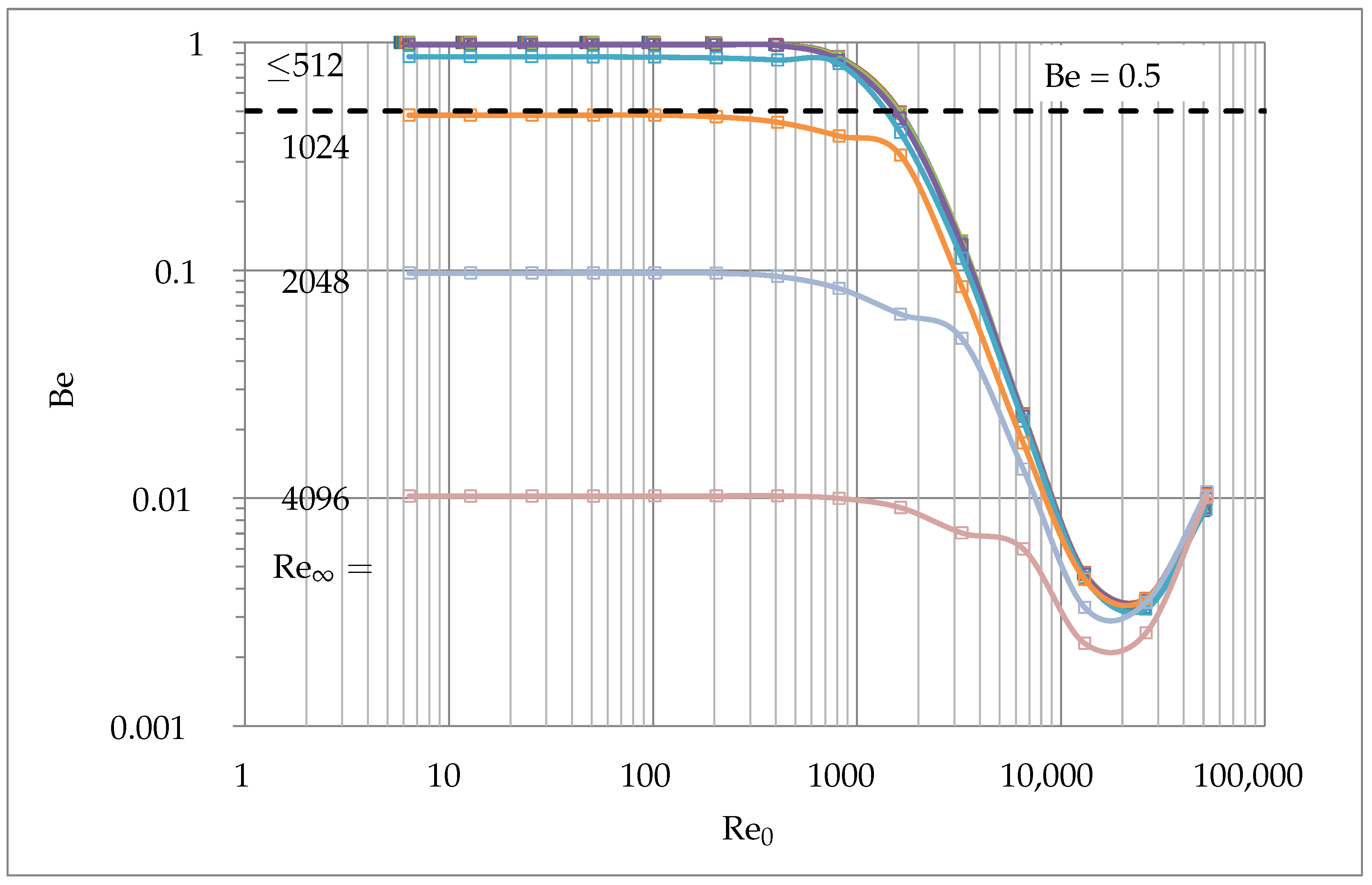
Figure 16 presents the Bejan number (Be) which was introduced by Paoletti
et al. [
33] and is defined as:
The range of the Bejan number is , where 0 is the limit at which the irreversibility is dominated by dissipation effects. At the irreversibility due to conduction dominates and at the irreversibility rates of dissipation and conduction are equal. The dashed line shows the equilibrium. For the range , corresponds exactly to . For the same equilibrium is reached at . For values the entropy generation due to dissipation is the dominating effect and no equilibrium is observed. The minima of Be is at with the magnitude for all . For all considered the behaviors are qualitatively similar to each other.
Figure 15.
Effect of and on .
Figure 15.
Effect of and on .
Figure 16.
Effect of and on Be.
Figure 16.
Effect of and on Be.
7.5. Information Regarding The Flow Field
In
Figure 17,
Figure 18 and
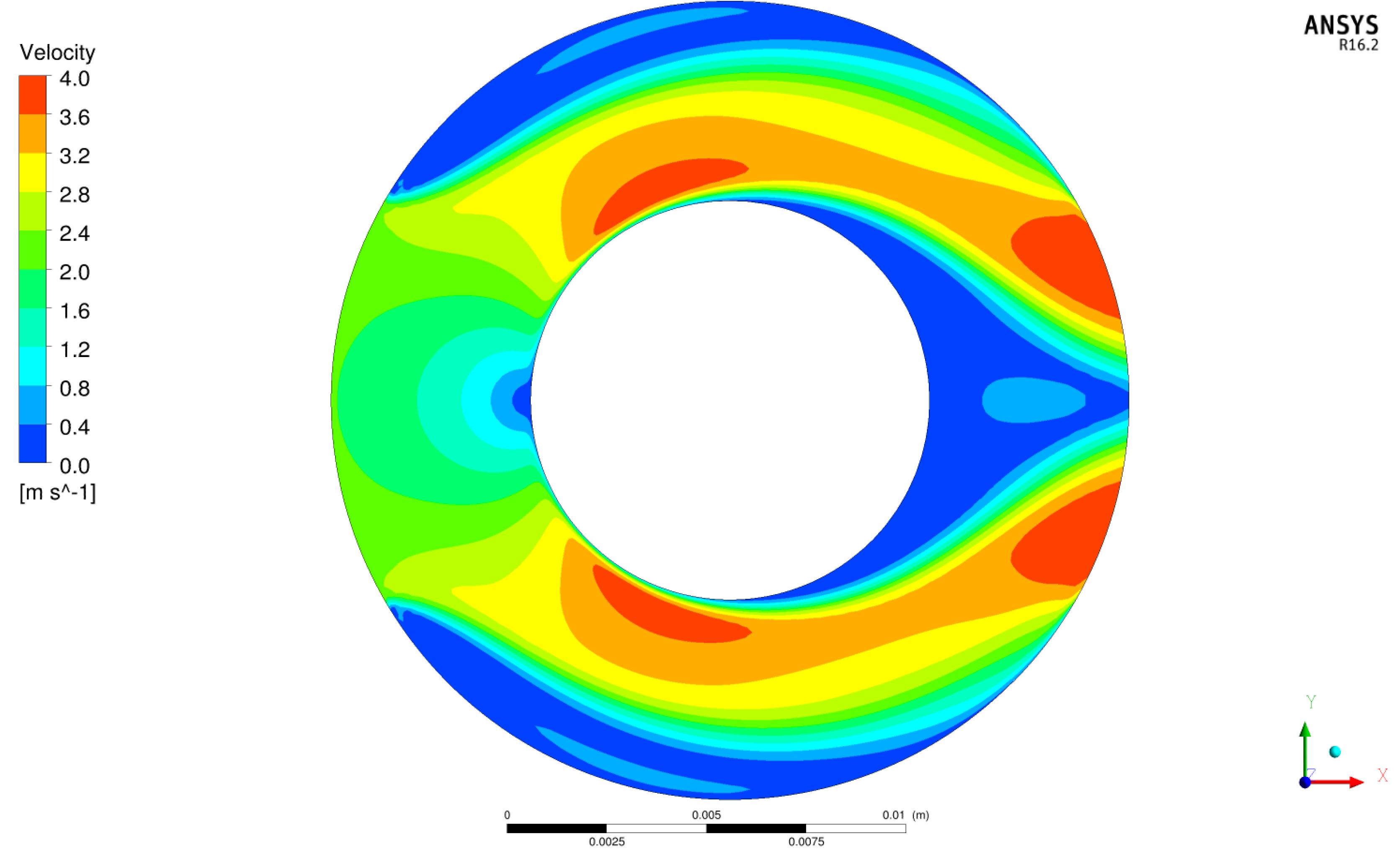
Figure 19 contour plots of velocity, temperature and total entropy generation are shown for the case
and
. Symmetric results are naturally obtained. High velocities are seen in
Figure 17 around the cylinder. In the near-wall region the velocity goes to zero due to the no-slip boundary condition.
Figure 17.
Contour plot of u for and .
Figure 17.
Contour plot of u for and .
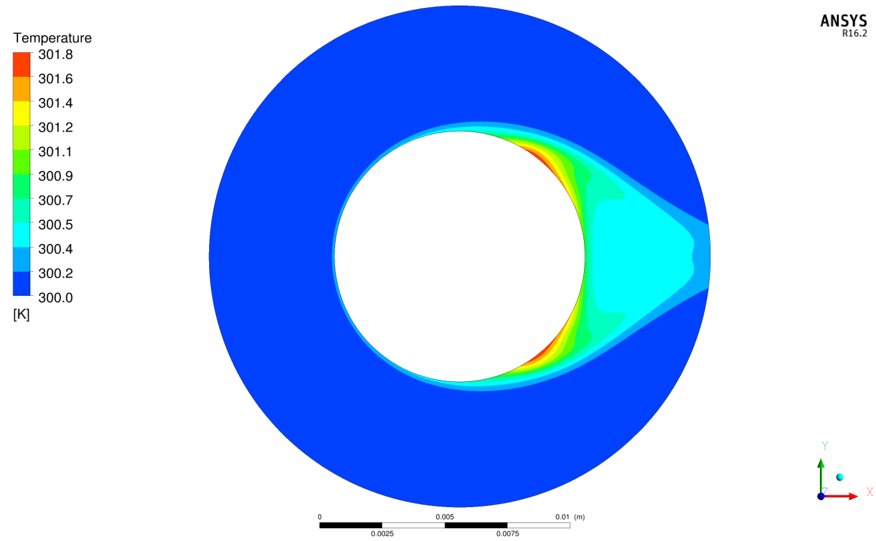
Figure 18.
Contour plot of T for and .
Figure 18.
Contour plot of T for and .
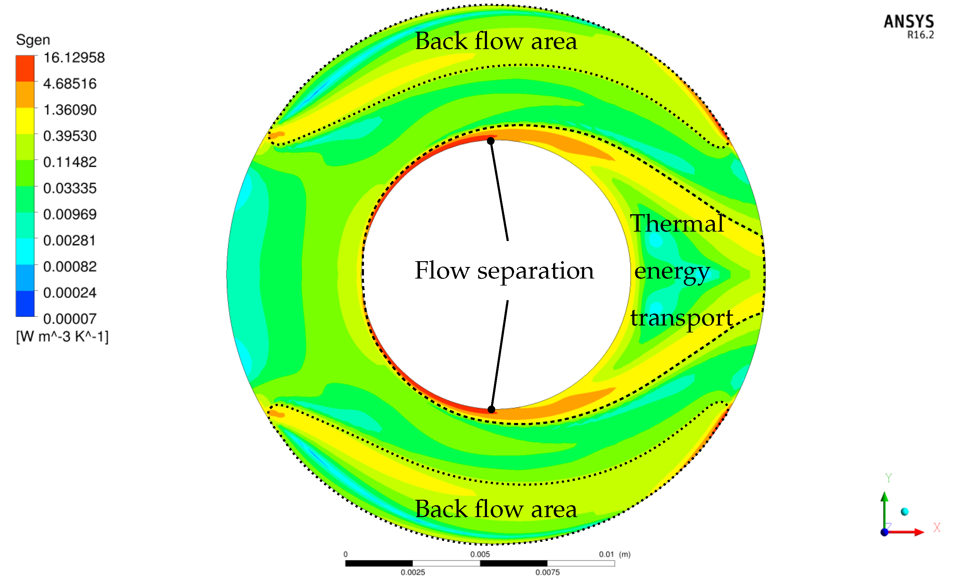
Between the rotating cylinder and the fixed sleeve, a back flow area exists along the sleeve’s wall (highlighted in
Figure 19). In this area the flow velocity is obviously very low. For a better thermal energy transport such areas should be avoided. Looking at the temperature contour plot in
Figure 18 the thermal energy transport downstream of the cylinder is clearly visible (highlighted in
Figure 19). High temperatures are found behind the rotating cylinder. The temperature gradients in the fluid are much smaller than along the solid-fluid interface. Due to that, most of the areas (in particular in front of, above and below the cylinder) convey no further information about the flow field when analyzing the temperature. Compared to the velocity contour plot, the temperature contour plot gives no useful information for optimizing the flow field. In
Figure 19 all information from the previously discussed variables (
u and
T) can be found by analyzing the entropy generation. The back flow area clearly appears, as well as the area of thermal energy transport downstream of the cylinder. In addition, the separation point along the rotating cylinder can be clearly detected.
Figure 19.
Contour plot of for and .
Figure 19.
Contour plot of for and .
Finally, the total volumetric entropy generation describes both entropy generation due to dissipation and due to conduction in one single value, as discussed in
Section 7.3. Based on this information, optimizing the sleeve shape to get a better cooling of the rotating cylinder becomes possible.
8. Conclusions
Numerical investigations of entropy generation relying on a canonical configuration have been carried out successfully. Thanks to this simplified configuration the complex flow processes that occur in a real alternator system can be simulated in an efficient manner. By reducing the numerical effort, the identification of suitable indicators such as entropy generation becomes possible. The first and second law of thermodynamics have been used in combination with numerical simulations to demonstrate the advantage of this new concept. After grid-independence tests and code verification, promising results have been obtained.
A constant wall heat flux along the cylinder was considered for all simulations. The oncoming flow enters the domain between the static sleeve and the rotating cylinder through an opening angle .
The entropy generation due to dissipation shows a smooth variation when varying oncoming flow velocity (thus ) and tangential velocity (connected to ). When increasing Reynolds number ( or ), increases as well. Therefore, the minimum of is found at the lowest Reynolds numbers. These results correlate with the volumetric flow rate measured along the outlet of the canonical configuration.
The volumetric entropy generation due to conduction decreases when increasing the velocity of incoming flow . The minimum is found at for all simulations considered. Below this value, the flow field is too slow for an optimal thermal energy transport. Above this value the viscous effects increase and, therefore, the temperature difference between fluid and solid gets smaller. These results correlate with the dimensionless temperature difference .
The total volumetric entropy generation shows a similar behavior as the entropy generation due to conduction for all . Here, the minima is at . If is larger, the total entropy generation becomes dominated by the entropy generation due to dissipation and has therefore its minima at small and values.
Considering the contour plots it can be seen, that the total entropy generation contains in a lumped form the information from velocity and temperature, which is very important, for instance in connection with recirculation areas. In addition, the entropy generation enables a physically-based comparison between two competing properties measured with the same unit. Based on entropy generation, optimizing cooling properties of electric machines should be possible. With this knowledge, promising regions for optimization can be located.
The next step consists in carrying out a design optimization of the canonical configuration based on the entropy generation and on the results discussed in this work. Finally, a real, industrial configuration will be considered in the same manner.


