2.1. Entropy, Dimension and Excess Entropy
Starting point is a (in general) vector valued stationary time series
. It is used to reconstruct the phase space of the underlying dynamical system by using delay embedding:
. If the original time series was
dimensional the reconstructed phase space will be of dimension
. More general embeddings are also possible, e.g., involving different delays or different embedding dimensions for each component of the time series. In the following, we will only consider the case
,
i.e., scalar time series. The generalization to vector-values time series is straight forward. Let us assume that we are able to reconstruct approximately the joint probability distribution
in a reconstructed phase space. Then we can characterize its structure using measures from information theory. Information theoretic measures represent a general and powerful tool for the characterization of the structure of joint probability distributions [
20,
21]. The uncertainty about the outcome of a single measurement of the state,
i.e., about
is given by its
entropy. For discrete-valued random variable
X with values
and a probability distribution
it is defined as
An alternative interpretation for the entropy is the average number of bits required to encode a new measurement. In our case, however, the
are considered as continuous-valued observables (that are measured with a finite resolution). For continuous random variables with a probability density
one can also define an entropy, the
differential entropyHowever, it behaves differently than its discrete counterpart: It can become negative and it will get even minus infinity if the probability measure for
X is not absolutely continuous with respect to the Lebesgue measure—for instance, in the case of the invariant measure of a deterministic system with an attractor dimension smaller than the phase space dimension. Therefore, when using information theoretic quantities for characterizing dynamical systems researchers often prefer using the entropy for discrete-valued random variables. In order to use them for dynamical systems with continuous variables usually either partitions of the phase space or entropy-like quantities based on coverings are employed. These methods do not explicitly reconstruct the underlying invariant measure, but exploit the neighbor statistics directly. Alternatively one could use direct reconstructions using kernel density estimators [
22] or methods based on maximizing relative entropy [
23,
24] to gain parametric estimates. These reconstructions, however, will always lead to probability densities, and are not suitable for reconstructing fractal measures which appear as invariant measures of deterministic systems.
In this paper, we use estimators based on coverings,
i.e., correlation entropies [
25] and nearest neighbors based methods [
26] considered in
Section 2.3 below. For the moment let us consider a partition of the phase space into hypercubes with side-length
ϵ. For a more general definition of an
ϵ-partition see [
27]. In principle one might consider scaling the different dimensions of
differently, but for the moment we assume that the time series was measured using an appropriate rescaling. The entropy of the state vector
observed with a
ε-partition will be denoted in the following as
with
ϵ parameterizing the resolution.
How does the entropy change if we change
ε? The uncertainty about the potential outcome of a measurement will increase if the resolution of the measurement is increased, because of the larger number of potential outcomes. If
is a m-dimensional random variable and distributed according to a corresponding probability density function
we have asymptotically for
see ([
27] or [
28] (ch. 8, p. 248, theorem 8.3.1)).
This is what we would expect for a stochastic system. However, if we observe a deterministic system the behavior of an observable depends how its dimension relates to the attractor dimension. If the embedding dimension is smaller than the attractor dimension the deterministic character will not be resolved and Equation (
2) still applies. However, if the embedding dimension is sufficiently high (
[
29]) then instead of a density function
we have to deal with a
D-dimensional measure
and the entropy will behave as
If an behavior such as in Equations (2) or (3) is observed for a range of ϵ values we will call this range a stochastic or deterministic scaling range, respectively.
Conditional entropy and mutual information Let us consider two discrete-valued random variables
X and
Y with values
and
, respectively. Then the uncertainty of a measurement of
X is quantified by
. Now we might ask, what is the average remaining uncertainty about
X if we have seen already
Y? This is quantified by the
conditional entropy The reduction of uncertainty about
X knowing
Y is the information that
Y provides about
X and is called the
mutual information between
X and
YHaving defined the
ε-dependent state entropy
we can now ask, how much information the present state contains about the state of the system at the next time step. The answer is given by the mutual information between
and
:
Using Equation (
2) one see, that for stochastic systems the mutual information will remain finite In the limit
and can be expressed by the differential entropies:
Note that this mutual information is invariant with respect to coordinate transformation of the system state,
i.e., if
is a continuous and invertible function, then
However, in the case of a deterministic system, the mutual information will diverge
This is reasonable behavior because in principle the actual state contains an arbitrary large amount of information about the future. In practice, however, the state is known only with a finite resolution determined by the measurement device or the noise level.
Predictive information, excess entropy and entropy rate The unpredictability of a time series can be characterized by the conditional entropy of the next state given the previous states. In the following we will use an abbreviated notation for these conditional entropies and the involved entropies:
The
entropy rate ([
28] see (ch. 4.2)) is this conditional information if we condition on the infinite past
In the following we assume stationarity,
i.e., we have no explicit time dependence of the joint probabilities and therefore also of the entropies. Moreover, if it is clear from the context, which stochastic process is considered, we will write
and
instead of
and
, respectively and it holds
For deterministic systems the entropy rate will converge in the limit
to the Kolmogorov-Sinai (KS-)entropy [
30,
31] which is a dynamical invariant of the system in the sense that it is independent on the specific state space reconstruction. Moreover, already for finite
,
will not depend on
ε for sufficiently small
ε because of Equation (
3).
To quantify the amount of predictability in a state sequence one might consider subtracting the unpredictable part from the total entropy of a state sequence. By doing this one ends up with a well known complexity measure for time series, the
excess entropy [
14,
15] or
effective measure complexity [
16]
with
The excess entropy provides a lower bound for the amount of information necessary for an optimal prediction. For deterministic systems, however, it will diverge because
will behave according to Equation (
3) and
will become
ϵ-independent for sufficiently large
m and small
ϵ, respectively
with
D being the attractor dimension.
The
predictive information [
13] is the mutual information between the semi-infinite past and the future time series
with
If the limits Equations (14) and (17) exist the predictive information
is equal to the excess entropy
. For the finite time variants in general
:
However, if the system is Markov of order p the conditional probabilities will only depend on the previous p time steps, , hence for and therefore .
2.2. Decomposing the Excess Entropy for Continuous States
In the literature [
13,
15,
16] both the excess entropy and the predictive information were studied only for a given partition—usually a generating partition. Thus, using the excess entropy as a complexity measure for continuous valued time series has to deal with the fact that its value will be different for different partitions—even for different generating ones.
In Equation (
16) we have seen that the excess entropy for deterministic systems becomes infinite in the limit
. The same applies to the predictive information defined in Equation (
18). Moreover, we have seen that the increase of these complexity measures with decreasing
ε is controlled by the attractor dimension of the system. Does this means that in the case of deterministic systems the excess entropy as a complexity measure reduces to the attractor dimension? Not completely. The constant in Equation (
16) reflects not only the scale of the signal, but also statistical dependencies or memory effects in the signal, in the sense that it will be larger if the conditional entropies converge slower towards the KS-entropy.
How can we separate the different contributions? We will start by rewriting Equation (
15) as a sum. Using the conditional entropies (Equation (
13)) we get
Using the differences between the conditional entropies
the excess entropy can be rewritten as
Note that the difference
is the conditional mutual information
It measures dependencies over
m time steps that are not captured by dependencies over
time steps. In other words, how much uncertainty about
can by reduced if in addition to the
step past also the
m th is taken into account. For a Markov process of order
m-the
vanish for
. In this case the sum in Equation (
20) contains only a finite number of terms. On the other side truncating the sum at finite
m could be interpreted as approximating the excess entropy by the excess entropy of an approximating Markov process. What can be said about the scale dependency of the
? From Equations (2) and (3) follows that
for
and
for
. Using this and Equation (
19) we have to distinguish four cases for deterministic systems. Note that
denotes the fractal part of the attractor dimension.
Thus the sum Equation (
20) can be decomposed into three parts:
with the
ε dependence showing up only in the middle term (MT):
with
denoting the length scale where the deterministic scaling range starts. Therefore we have decomposed the excess entropy in three terms: Two ideally
ε independent terms and one
ε-dependent term. The first term
will be called “state complexity” in the following because it is related to the information encoded in the state of the system. The constant
c was added here in order to ensure that the
ϵ-dependent term vanishes at
—the beginning of the deterministic scaling range. The second
ε-independent term
will be called “memory complexity” because it is related to the dependencies between the states on different time steps. What we call “state” in this context is related to the minimal embedding dimension to see the deterministic character of the dynamics which is
[
29]. In order to be able to get a one to one reconstruction of the attractor a higher embedding dimension might be necessary [
32]. Both
ε-independent terms together we will call “core complexity”
So far we only addressed the case of a deterministic scaling range. In the case of a noisy chaotic system we have to distinguish two
ε regions: the deterministic scaling range described above and the noisy scaling range with
with
determined by the noise level. In the stochastic scaling range all
become
ε-independent and the decomposition Equation (
22) seems to become unnecessary. This is not completely the case. Let us assume that the crossover between the two regions happens at a length scale
. Moreover, let us assume that for sufficiently large
m we have in the deterministic scaling range
(see
Section 2.5 for an example). Then we have
which allows to express the cross-over scale
in terms of the KS-entropy and the noise level related continuous entropy
Moreover, the excess entropy in the
deterministic scaling range will behave as
Evaluating this expression at the crossover length scale
allows to express the value of the excess entropy in the
stochastic scaling range as
In particular, this expression shows that decreasing the noise level, which increases
, will increase the asymptotic value of the excess entropy for noisy systems. Thus, an increased excess entropy or predictive information for a fixed length scale or partition can be achieved in many ways:
by increasing dimension D of the dynamics
by decreasing the noise level
by increasing the amplitude
by increasing the state complexity
by increasing the correlations measured by the “memory” complexity, i.e., by increasing the predictability
by decreasing the entropy rate , i.e., by decreasing the unpredictability
Naturally, the effect of the noise level will be observed in the stochastic scaling range only. In practice there might be more than one deterministic and stochastic scaling range or even no clear scaling range at all. How we will deal with these cases will be described below when we introduce our algorithm.
2.3. Methods for Estimating the Information Theoretic Measures
Reliably estimating entropies and mutual information is very difficult in high-dimensional spaces due to the increasing bias of entropy estimates. Therefore we will employ two different approaches. On the one hand we will use an algorithm for the estimation of the mutual information proposed by Kraskov
et al. [
26] based on nearest neighbor statistics which allows to reduce the bias by employing partitions of different sizes in spaces of different dimensions. On the other hand we calculate a proxy for the excess entropy using correlation entropies [
25] of order
. These are related to the Rényi entropies of second order and the correlation sum provides an unbiased estimator. Both methods do not require binning but differ substantially in what they compute.
Estimation via local densities from nearest neighbor statistics (KSG) The most common approach to estimate information quantities of continuous processes, such as the mutual information, is to calculate the differential entropies (1) directly from the nearest neighbor statistics. The key idea is to use nearest neighbor distances [
33,
34,
35] as proxies for the local probability density. This method corresponds in a way to an adaptive bin-size for each data point. For the mutual information
(required e.g., to calculate the PI (Equation (
18))), however, it is not recommended to naively calculate it directly from the individual entropies of
X,
Y and their joint
because they may have very dissimilar scale such that the adaptive binning leads to spurious results. For that reason a new methods was proposed by Kraskov
et al. [
26], that we call
KSG, which only uses the nearest neighbor statistics in the joint space. We denote
the mutual information estimate where
k nearest neighbors where used for the local estimation.
The length scale on which the mutual information is estimated by this algorithm depends on the available data. In the limit of infinite amount of data
for
. However, in order to evaluate the quantity at a certain length scale (similar to
ε above) and assuming the same underlying space for
X and
Y, noise of strength
η is added to the data resulting in
where
is the uniform distribution in the interval
. The idea of adding noise is to make the processes X and Y independent within neighborhood sizes below the length scale of the noise. In this way only the structures above the added noise-level contribute to the mutual information. Note that for small
η the actual scale (
k-neighborhood size) may be larger due to sparsity of the available data.
Estimation via correlation sum The correlation sum is one of the standard tools in nonlinear time series analysis [
36,
37]. Normally it is used to estimate the attractor dimension. However, it can also be used to provide approximate estimates of entropies and derived quantities such as the excess entropy. The correlation entropies for a random variable
with measure
are defined as [
25]
where
is the “ball” at
with radius
ε. For
Equation (
32) becomes
. The integral in this formula is also known as “correlation integral”. For
N data points
it can be estimated using the correlation sum, which is the averaged relative number of pairs in an
ε-neighborhood [
36,
37],
Θ denotes the Heaviside function
Then the correlation entropy is
For sufficiently small
ε it behaves as
with
being the correlation dimension of the system [
38]. A scale dependent correlation dimension can be defined as difference quotient
For a temporal sequence of states (or state vectors)
we can now define block entropies
by using
-dimensional delay vectors
. Now, we can define also the quantities corresponding to conditional entropies and to the excess entropy using the correlation entropy
We expect the same qualitative behavior regarding the ε-dependence of these quantities as for those based on Shannon entropies, see Equations (11) and (15). Quantitatively there might be differences, in particular for large ε and strongly non-uniform measures.
A comparison of the two methods with analytical results are given in the
Appendix A, where we find a good agreement. Although, the KSG method seems to underestimate the mutual information for larger embeddings (higher dimensional state space). The correlation integral method uses a unit ball of diameter
whereas the KSG method measures the size of the hypercube enclosing
k neighbors where the data was subject to additive noise in the interval
. Thus comparable results are obtained with
.
2.4. Algorithm for Excess Entropy Decomposition
We are now describing the algorithm used to compute the proposed decomposition of the excess entropy in
Section 2.2. The algorithm is composed of several steps: preprocessing, determining the middle term (MT) (Equation (
23)), determining the constant in MT, and the calculation of the decomposition and of quality measures.
Preprocessing: Ideally the
curves are composed of straight lines in a log-linear representation,
i.e., of the form
. We will refer to
s as the slope (it is actually the inverted slope). Thus we perform fitting, that attempts to find segments following this form, details are provided in the
Appendix B. Then the data is substituted by the fits in the intervals where the fits are valid. As for very small scales the
become very noisy we extrapolate below the fit with the smallest scale. In addition we calculate the derivative
in each point, either from the fits (
s, where available) or from finite differences of the data (using 5 points averaging).
Determining MT: In theory only two
should have a non-zero slope at each scale
ε, see Equation (
21). However, in practice we often have more terms, such that we need to find for each
ε the maximal range
, where
,
i.e., the slope is larger than the threshold
. However, this is only valid for deterministic scaling ranges. In stochastic ranges all
should have zero slope. We introduce a measure of stochasticity, defined as
which is 0 for purely deterministic ranges and 1 for stochastic ones. The separation between state and memory complexity is then inherited from the next larger deterministic range. Thus if
we use
at
, where
. Note that the here algorithmically defined
is not necessarily equal to the
defined above Equation (
28) for an ideal-typical noisy deterministic system.
Determining the constant in MT: In order to obtain the scale-invariant constant
c of the MT, see Equation (
23), we would have to define a certain length scale
. Since this cannot be done robustly in practice (in particular because it may not be the same
for each
m) we resort to a different approach. The constant parts of the
terms in the MC can be determined from plateaus on larger scales. Thus, we define
, where
is smallest scale
where we have a near-zero slope,
i.e.,
. In case there is no such
then
.
Decomposition and quality measures: The decomposition of the excess entropy follows Equations (24) and (25) with
and
used for splitting the terms:
In addition we can compute different quality measures to indicate the reliability of the results, see
Table 1.
Table 1.
Quality measures for decomposition algorithm. We use the Iverson bracket for Boolean expression: and . They are all normalized to where typically 0 is the best score and 1 is the worst.
Table 1.
Quality measures for decomposition algorithm. We use the Iverson bracket for Boolean expression: and . They are all normalized to where typically 0 is the best score and 1 is the worst.
| Quantity | Definition | Description |
|---|
| κ=stochastic(ε) | | 0: fully deterministic, 1: fully stochastic at ε |
| % negative(ε) | | percentage of negative |
| % no fits(ε) | | percentage of where no fit is available |
| % extrap.(ε) | | percentage of that where extrapolated |
2.5. Illustrative Example
To get an understanding of the quantities, let us first apply the methods to the Lorenz attractor, as a deterministic chaotic system, and to its noisy version as a stochastic system.
Deterministic system: Lorenz attractor The Lorenz attractor is obtained as the solution to the following differential equations:
integrated with standard parameters
,
,
.
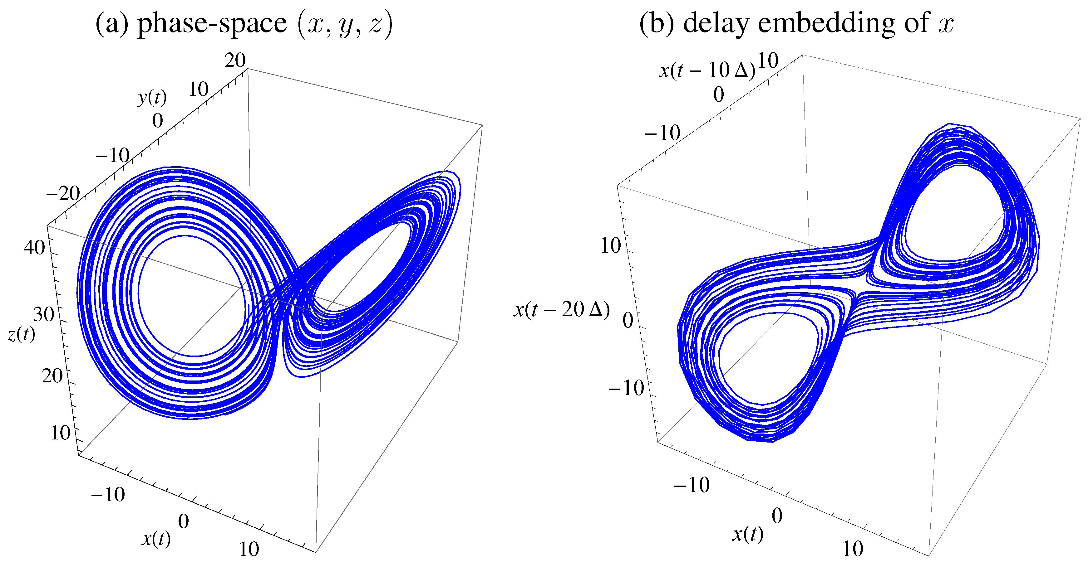
Figure 1 displays the trajectory in phase-space (
) and using delay embedding of
using
and time delay is
(for sampling time
). The equations where integrated with Runge-Kutta fourth order with step size
. An alternative time delay may be obtained from first minimum of mutual information as a standard choice [
39,
40], which would be
, but
yields clearer results for presentation.
Figure 1.
Lorenz attractor with standard parameters. (a) Trajectory in state space . (b) Embedding of x with , time-delay , and .
Figure 1.
Lorenz attractor with standard parameters. (a) Trajectory in state space . (b) Embedding of x with , time-delay , and .
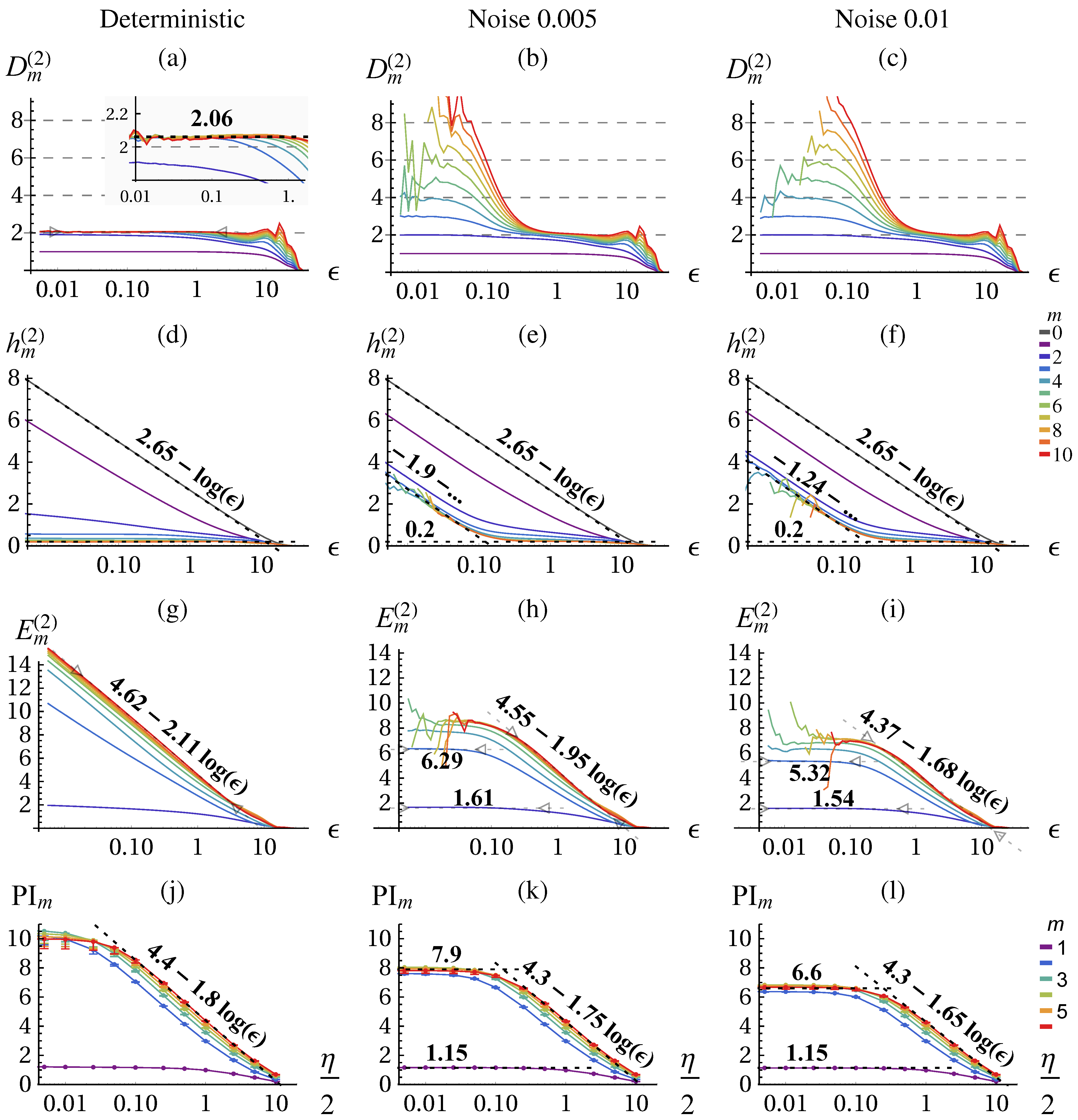
The result of the correlation sum method using TISEAN [
41] is depicted in
Figure 2 for
data points. From the literature, we know that the chaotic attractor has a fractal dimension of
[
38] which we can verify with the correlation dimension
, see
Figure 2a for
and small
ε. The conditional
(d) becomes constant and identical for larger
m. The excess entropy
(g) approaches the predicted scaling behavior of:
(Equation (
16)) with
and
. The predictive information
. (j) shows the same scaling behavior on the coarse range but with a smaller slope and saturates at small
ε.
Stochastic system: noisy Lorenz attractor In order to illustrate the fundamental differences between deterministic and stochastic systems when analyzed with information theoretic quantities we consider now the Lorenz dynamical system with dynamic noise (additive noise to the state (
) in Equations (38)–(40) before each integration step) as provided by the TISEAN package [
41]. The dimension of a stochastic systems is infinite,
i.e., for embedding
m the correlation integral yields the full embedding dimension as shown in
Figure 2b,c for small
ε.
On large scales the dimensionality of the underlying deterministic system can be revealed to some precision either from
or from the slope of
or PI. Thus, we can identify a determinstic and a stochastic scaling range with different qualitative scaling behavior of the quantities. In contrast with the deterministic case, the excess entropy converges in the stochastic scaling range and no more contribution from
are observed as shown in
Figure 2h,i. By measuring the
ε-dependence (slope) we can actually differentiate between deterministic and stochastic systems and scaling ranges, which is performed by the algorithm
Section 2.4 and presented in
Figure 3. The predictive information
Figure 2k,l again yields a lower slope, meaning a lower dimension estimate, but is otherwise consistent. However, it does not allow to safely distinguish determinstic and stochastic systems, because it always saturates due to the effect of finite amount of data.
Figure 2.
Correlation dimension
(Equation (
34)) (
a)–(
c), conditional block entropies
(Equation (
35)) (
d)–(
f), excess entropy
(Equation (36) (
g)–(
i), and predictive information
(Equation (
18)) (
j)–(
l) of the Lorenz attractor estimated with the correlation sum method (
a)–(
i) and KSG (
j)–(
l) for the deterministic system (first column) and with absolute dynamic noise
, and
(second and third column respectively). The error bars in (
j)–(
l) show the values calculated on half of the data. All quantities are given in nats (natural unit of information with base
e) and in dependence of the scale (
ε,
η in space of
x (Equation (
38))) for a range of embeddings
m, see color code. In (
d)–(
f) the fits for
allow to determine
and for
give
and
, Equations (27)–(30). Parameters: delay embedding of
x with
.
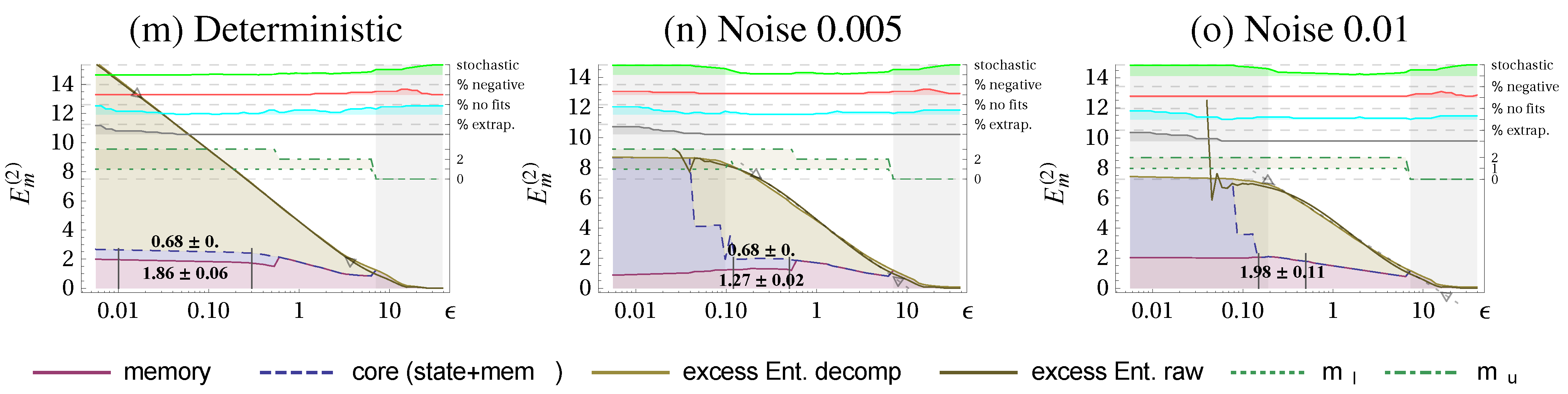
Figure 3.
Excess Entropy decomposition for the Lorenz attractor into state complexity (blue shading), memory complexity (red shading), and
ε-dependent part
(beige shading) (all in nats). Columns as in
Figure 2: deterministic system (a), with absolute dynamic noise
(b), and
(c). A set of quality measures and additional information is displayed on the top using the right axis.
and
refer to the terms in
(Equation (
37)). Scaling ranges that are identified as stochastic are shaded in gray (stochastic indicator
). In manually chosen ranges, marked with vertical black lines, we evaluate the mean and standard deviation of the memory- and state complexity. Parameters:
.
Let us now consider the decomposition of the excess entropy as discussed in
Section 2.2 and
Section 2.4 to see whether the method is consistent.
Figure 3 shows the scale-dependent decomposition together with the determined stochastic and deterministic scaling ranges. The resulting values for comparing the determinstic scaling range are given in
Table 2 and reveal, that the
decreases for increasing noise level similarly as the constant reduces. This is a consistency check because the intrinsic scale (amplitudes) of the deterministic and noisy Lorenz system are almost identical. We also checked the decomposition for a scaled version of the data where we found the same values state-, memory- and core complexity. We see also that the state complexity
vanishes for larger noise, because the dimension drops significantly below 2, where we have no summands in the state complexity and the constant
is also 0.
Table 2.
Decomposition of the excess entropy for the Lorenz system. Presented are the unrefined constant and dimension of the excess entropy, the state-, memory-, and core complexity (in nats) determined in the deterministic scaling range, see
Figure 3.
Table 2.
Decomposition of the excess entropy for the Lorenz system. Presented are the unrefined constant and dimension of the excess entropy, the state-, memory-, and core complexity (in nats) determined in the deterministic scaling range, see Figure 3.
| | | Determ. | Noise | Noise | Noise |
|---|
| Equation (16) | D | 2.11 | 1.95 | 1.68 | 1.59 |
| Equation (16) | | 4.62 | 4.55 | 4.37 | 4.21 |
| Equation (27) | | 0 | 0.12 | 0.23 | 0.45 |
| Equation (24) | | 0.68 ± 0 | 0.68 ± 0 | 0 | 0 |
| Equation (25) | | 1.86 ± 0.06 | 1.27 ± 0.02 | 1.98 ± 0.11 | 1.2 ± 0.1 |
| Equation (26) | | 2.54 ± 0.06 | 1.95 ± 0.02 | 1.98 ± 0.11 | 1.2 ± 0.1 |
To summarize, in deterministic systems with a stochastic component, we can identify different ε-ranges (scaling ranges) within which stereotypical behaviors of the entropy quantities are found. This allows us to determine the dimensionality of the deterministic attractor and decompose the excess entropy in order to obtain two ε-independent complexity measures.


