Article

Analysis of Neural Oscillations on Drosophila’s Subesophageal Ganglion Based on Approximate Entropy

1
Department of Biomedical Engineering, Zhongshan School of Medicine, Sun Yat-sen University, Guangzhou 510080, China
2
Department of Anatomy and Neurobiology, Zhongshan School of Medicine, Sun Yat-Sen University, Guangzhou 510080, China
3
College of Medical Engineering and Technology, Xinjiang Medical University, Urumqi 830011, China
4
Department of Neurology, First Affiliated Hospital of Sun Yat-sen University, Guangzhou 510080, China
5
College of Public Health, Xinjiang Medical University, Urumqi 830011, China
*
Author to whom correspondence should be addressed.
Entropy 2015, 17(10), 6854-6871; https://doi.org/10.3390/e17106854
Submission received: 13 August 2015 / Accepted: 30 September 2015 / Published: 10 October 2015

Abstract

:
The suboesophageal ganglion (SOG), which connects to both central and peripheral nerves, is the primary taste-processing center in the Drosophila’s brain. The neural oscillation in this center may be of great research value yet it is rarely reported. This work aims to determine the amount of unique information contained within oscillations of the SOG and describe the variability of these patterns. The approximate entropy (ApEn) values of the spontaneous membrane potential (sMP) of SOG neurons were calculated in this paper. The arithmetic mean (MA), standard deviation (SDA) and the coefficient of variation (CVA) of ApEn were proposed as the three statistical indicators to describe the irregularity and complexity of oscillations. The hierarchical clustering method was used to classify them. As a result, the oscillations in SOG were divided into five categories, including: (1) Continuous spike pattern; (2) Mixed oscillation pattern; (3) Spikelet pattern; (4) Busting pattern and (5) Sparse spike pattern. Steady oscillation state has a low level of irregularity, and vice versa. The dopamine stimulation can distinctly cut down the complexity of the mixed oscillation pattern. The current study provides a quantitative method and some critera on mining the information carried in neural oscillations.

1. Introduction

Drosophila, with a relatively simple brain structure, has become a model organism widely used in neurological studies [1]. Drosophila shares many deep homology genes with mammals [2]. A model system established based on it can provide an important access to studying the rules of nervous system activities as well as to conducting basic research on nervous system diseases like epilepsy and Parkinson’s disease [3,4].
The suboesophageal ganglion (SOG) is the primary taste-processing center in the Drosophila brain, and it is strongly related to feeding behavior. As the main projection area of the chemical sensory neurons in the limbs and mouthpart, the SOG contains about 6000 neurons located under the antennal lobe (AL) [5,6]. In recent years, extensive and in-depth studies on nuclei such as the mushroom body (MB) and AL, which are considered the senior central nervous system are widely conducted [7,8]. Unlike AL or MB, the SOG region does not simply receive and process chemical information of senses but also receives and transmits physical senses, and it can govern motion related neurons at the same time [9,10]. These diverse functions determine the diverse neural activities in SOG compared with other regions [11].
The patch clamp technique is a newly reformed dissection and record method of whole Drosophila brain. It enables the electrophysiological signals of a single cell to stay in an actual state [9], while it also greatly increases the amount of signals, making it more difficult to distinguishing the complicated and diverse oscillations. At present, identifying neuron oscillation only by judging its discharge quantity and whether it is spike or bursting fails to meet the demand of analysis [12].
Mathematical computing tools have been widely used in the analysis of neural signals [13,14,15,16,17]. One of them is approximate entropy (ApEn), a simple and straightforward nonlinear index, which can be used to measure the complexity of signals and quantify statistics [15,16,17,18]. In the past few years, ApEn has been extensively applied in the analysis of regularity and complexity of short-term physiological time series such as heart rate, blood pressure, and electroencephalogram signals [19]. For example, ApEn was used to recognize the alteration of different sleep stages [20] and serving as an assistant index to study hypothermia [21]. Some studies show that the dynamic alteration of ApEn can indicate the changes of regularity and complexity during the process of bursting discharge and spike emergence, and that it can help to identify different signals [18,22].
With the complicated and multitudinous oscillation patterns in the Drosophila’s SOG, proper classification of neuronal oscillations is essential for making further function studies [23]. In order to determine characteristics of these patterns in SOG, a novel approach to oscillation differentiation using the quantitative indicators of ApEn are presented. According to the three statistical indicators of ApEn, namely the arithmetic mean (MA), standard deviation (SDA) and the coefficient of variation (CVA), we clustered various oscillations in SOG into five typical categories and analyzed how the oscillations of the neuron changed while giving dopamine stimulation. The result illustrated that ApEn indicators can identify the changes of frequency of spikes and measure neural electrical signals, producing simple results.

2. Materials and Methods

2.1. Research Object

The current study used wild-type Drosophila melanogaster, which was took out two days before eclosion and conducted whole brain dissection using the method of Gu Huaiyu [24]. Drosophila stocks were reared on standard cornmeal agar medium supplemented with dry yeast at 24 °C and 60% relative humidity. Under such condition, Drosophila melanogaster produced new adults in 14 days. The 2-day-before-eclosion fly was identified by red eyes, transparent wing in the puparium. All experiments were performed on wild-type Caton-S female flies 2 days before exclusion.

2.2. Data Collection

The brains of flies were soaked in standard external sodium solution, which contains: 101 mM NaCl, 1 mM CaCl2, 4 mM MgCl2, 3 mM KCl, 5 mM glucose, 1.25 mM NaH2PO4 and 20.7 mM NaHCO3, pH 7.2, mosM 250. The internal solution contained the following: 102 mM K-gluconate, 0.085 mM CaCl2, 1.7 mM MgCl2, 17 mM NaCl, 0.94 mM EGTA and 8.5 mM Hepes, pH 7.2, mosM 235. The whole cell recording of the membrane activities was conducted with patch clamp technique. The neurons selected in SOG was of a diameter of more than 10 μm. The pipette resistance was 14–16 MΩ. The impedance of electrodes between entering water and contacting the cell was 11–15 MΩ. We located the electrode to the SOG region after forming a GΩ seal. The present study utilized two recording methods: (1) the spontaneous postsynaptic currents (sPSC) of the cell while clamping the voltage across the membrane at −70 mV was recorded, and the current changes of the neuron was observed; (2) the spontaneous membrane potential (sMP ) signals of the neuron at the gap-free mode of the clamp was recorded. All electrophysiological recordings were carried out using a BX51WI upright microscope (Olympus, Lehigh Valley, PA, USA). Signals were acquired with EPC10 amplifier (HEKA Elektronik, Lambrecht/Pfalz, Germany). The maximum sampling frequency was 20 KHz.

2.3. Data Processing

Electrophysiological data analysis was carried out using Clampfit 10.2 (Molecular Devices, Sunnyvale , CA, USA) and Matlab 2012b software (MathWorks, Natick, MA, USA). The selected data was from 12 selected recordings, among which 11 were under the stable natural condition while the other recordings were under dopamine treatment: Dopamine, whose concentration is 0.1 mM, is directly added into external solution. The recordings were counted for further analysis only if they were with typical waveforms.
Most neurons observed did not display apparent sPSC signals but had diverse sMP signals, so the sMP signals were analyzed. The maximum sampling frequency of sMP records was 20 KHz. Firstly, we sampled the signals to 2 KHz for data reduction, trying to keep balance with the judgment on oscillation patterns and simplifying the data. Secondly, we applied the 400 Hz Gaussian low-pass filter to minimize the interference of high-frequency noises and preserve the effective waveform information of the original data.

2.4. The ApEn Extraction Algorithm

The approximate entropy, which was proposed by Pincus as a model-independent measure of sequential irregularity, belongs to the field of information theory [18,25]. ApEn is to metric the probability of the emergence of new patterns and the amount of information can be computed in a finite sequence. Moreover, as ApEn embodies time patterns, it reflects the structural complexity of the data by indicating how the amount of repetitive patterns changes over the number of dimensions [26,27]. Neuronal electrical activities have often been deemed as nonperiodic and irregular [28,29]. Some studies have used information theory to assess the coding of task condition in spike rate, discharge irregularity, and proposed that the spike irregularity may reflect coding information [30].
ApEn algorithm has some anti-noise ability itself, and thus effect of different filtering methods can be reduced [19,31]. The amount of data is not so demanding (500–4000 points is generally enough) and some fast computation of ApEn has been developed, which makes the execution time shorter than other nonlinear algorithm [32,33].
Given a time series {u(i)}of size N, the ApEn value is calculated through the following steps [19]:
(1)
The sequence {u(i)} composes the m-dimensional vector X(i):
X(i) = [u(i), u(i + 1) … u(i + m − 1)], i = 1, 2, ..., N − m + 1
(2)
For every i value, the distance between vector X(i) and another vector X(j) is calculated:
d[X(i),X(j)] = max|u(i + k) − u(j + k)|, k = 0, 1, …, m − 1
(3)
Given the threshold value r ( r > 0), for each i value, statistical number of d [X (i), X (j)] < r is calculated .And the ratio of number to total N − m + 1 is called C i m ( r ) :
C i m ( r ) = number of  ( d [ X ( i ) , X ( j ) ] < r ) N m + 1
(4)
C i m ( r ) logarithm is obtained and the average i value is calculated, denoted as ϕ m ( r ) , namely:
ϕ m ( r ) = 1 N m + 1 i = 1 N m + 1 ln C i m ( r )
(5)
For m + 1, repeat from step 1 to step 4 and get ϕ m + 1 ( r ) ;
(6)
Finally, the results are as follows:
 ApEn(m,r) =  ϕ m ( r )   ϕ m + 1 ( r )
By comparison various setting [31], we set m = 2 and r = 0.25 SD(u) here (SD is the standard deviation). In the present study, 2000 sampling points were computed once, equal to ApEn of one second.

2.5. Evaluation of ApEn

The ApEn of different oscillation patterns differ from each other. The present study set the length of each calculated time window at N and the results of ApEn fluctuated over time. The current study introduced three statistical indicators to describe ApEn, namely the arithmetic mean of ApEn (MA), the standard deviation of ApEn (SDA) and the coefficient of variation of ApEn (CVA). The interval between two recordings is T, while the calculated oscillation length was 1 min.
The three statistical indicators of ApEn values are calculated by:
M A = 1 T / N A p E n T / N
S D A = 1 T / N ( A p E n M A ) 2 T N 1
C V A = SDA / MA
The mean value of ApEn can indicate integral complexity in a certain time series. The standard deviation indicates the degree of variation along with time .The variation coefficient, as the ratio of the standard deviation to the mean, is a relative indicator without dimension. More importantly, it can describe the relatively degree of variation while mean values are largely different. The more severe the fluctuation is, the larger the CVA will be.
The statistical significance of ApEn values was assessed using SPSS 16.0 software. For normality test of each group, the Kolmogorov-Smirnov tests were used with the significance level setting at p < 0.05. For the distribution test of ApEn values among different groups, the Kruskal-Wallis test was used with the significance level setting at p < 0.01. For the distribution tests of ApEn values among different oscillations within one group, the Kruskal-Wallis tests were used with the significance level setting at p < 0.01.

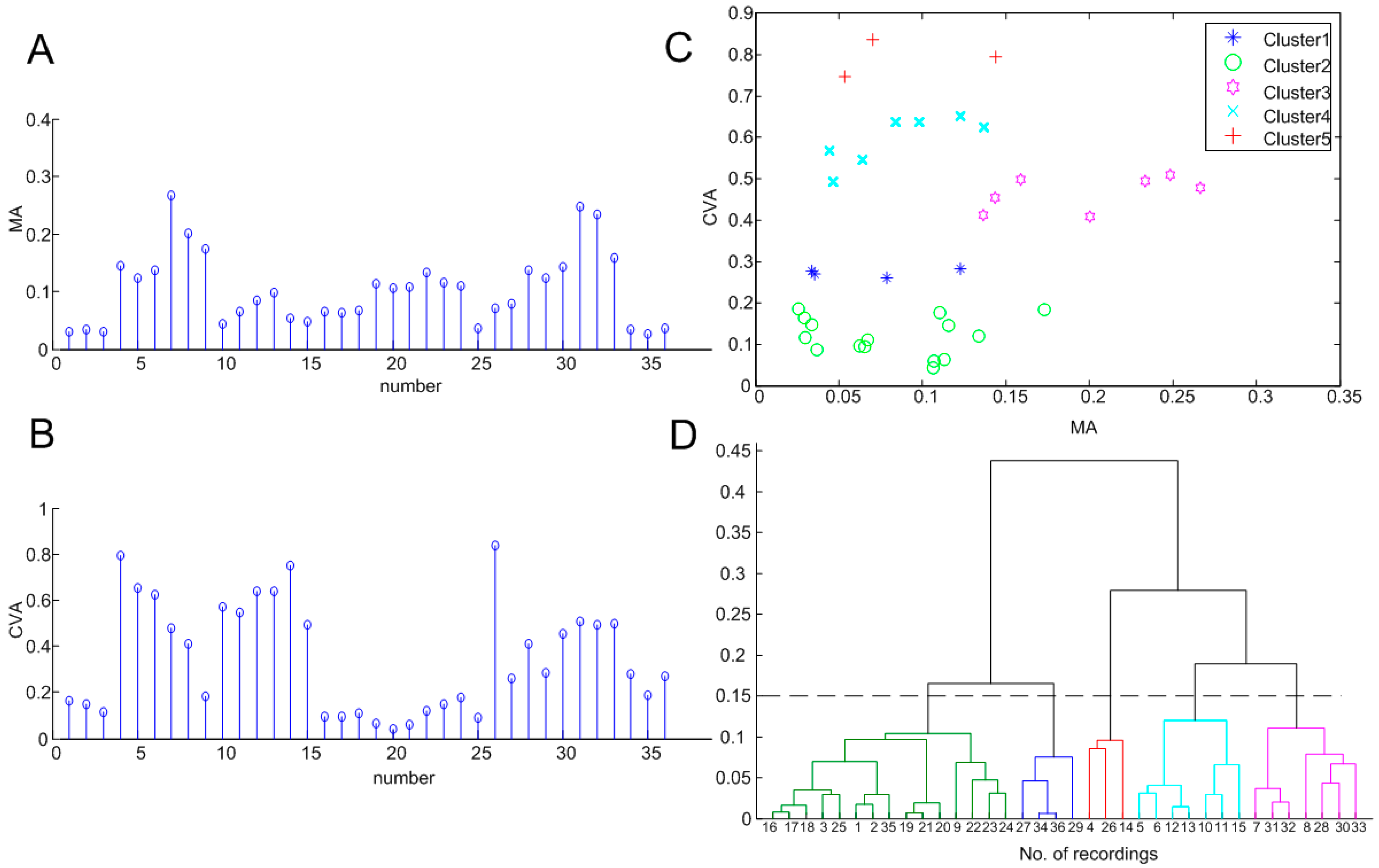
2.6. Clustering Analysis

Clustering analysis can automatically mine information from data to categorize observations. It has become an important tool for the analysis of neural activity characteristics [34]. As an unsupervised learning approach, clustering algorithms have also been widely applied to spike sorting [8,35]. To explore possible grouping of neurons according to the oscillation characteristics, the present study classified oscillation patterns with hierarchical clustering using MA and CVA as the two reference variables. The classification statistic was Squared Euclidean Distance and Average Linkage was performed. The classification statistic between sample i and sample j is defined as:
d i j = t = 1 2 ( x i t x j t ) 2
The distance between group p and group q is defined as:
D p q 2 = x i p x j q   d i j 2 / N P N q
Np and Nq are the numbers of elements in group p and group q respectively. In fact, various clustering were performed during the test and the above two methods were chosen because they came up with the best description of the common characteristics of oscillations.

3. Results

3.1. Statistical Indicators of Oscillation

To study the changes of oscillation over time, we focused on the time series during conversion of oscillatory states. Here, we take the typical continuous spike oscillation for example, which featured a slow depolarization process at the beginning stage, followed by a rapid process of depolarization and repolarization under gap free mode of the current clamp. The ApEn values were calculated firstly, based on which the three statistical indicators MA, SDA, and CVA were calculated for each one minute (Figure 1).
Figure 1. Three ApEn indicators of two different oscillation transition processes. (A) two types of oscillation transition. Type 1 shows a stable and continuous spike potential in 0–10 min, and it started to decay after 10 min. Type 2 shows the transition period lasted for roughly 0–8 min, followed by stable and continuous spike potential; (B) the corresponding variation tendencies of the three ApEn indicators of transition type 1; (C) the corresponding variation tendencies of the three ApEn indexes of transition type 2.
Entropy 17 06854 g001
With the disappearance of neuron spike potential, the discharge activity is weakened, which is manifested by the decrease of spike amplitude and discharge frequency, as well as the increase of the MA and the drop of the CVA. In Figure 1A, type1, from the stable and continuous spike stage to a transition period after 10 min, the MA rose from 0.1 to 0.4, the SDA also increased with mild fluctuation, and the CVA displayed an evident downtrend from 0.9 to 0.3 (Figure 1B). During the transition from sparse spike pattern to continuous spike activity (Figure 1A type 2), the MA decreased from 0.4 to below 0.1. When the neuron returned to a normal discharge state, the MA stayed at a relatively low level of 0.05. At the same time, the SDA dropped and leveled out at about 0.05. The CVA increased to a peak of 0.8 from 0.4, and fluctuated in a certain range afterwards.

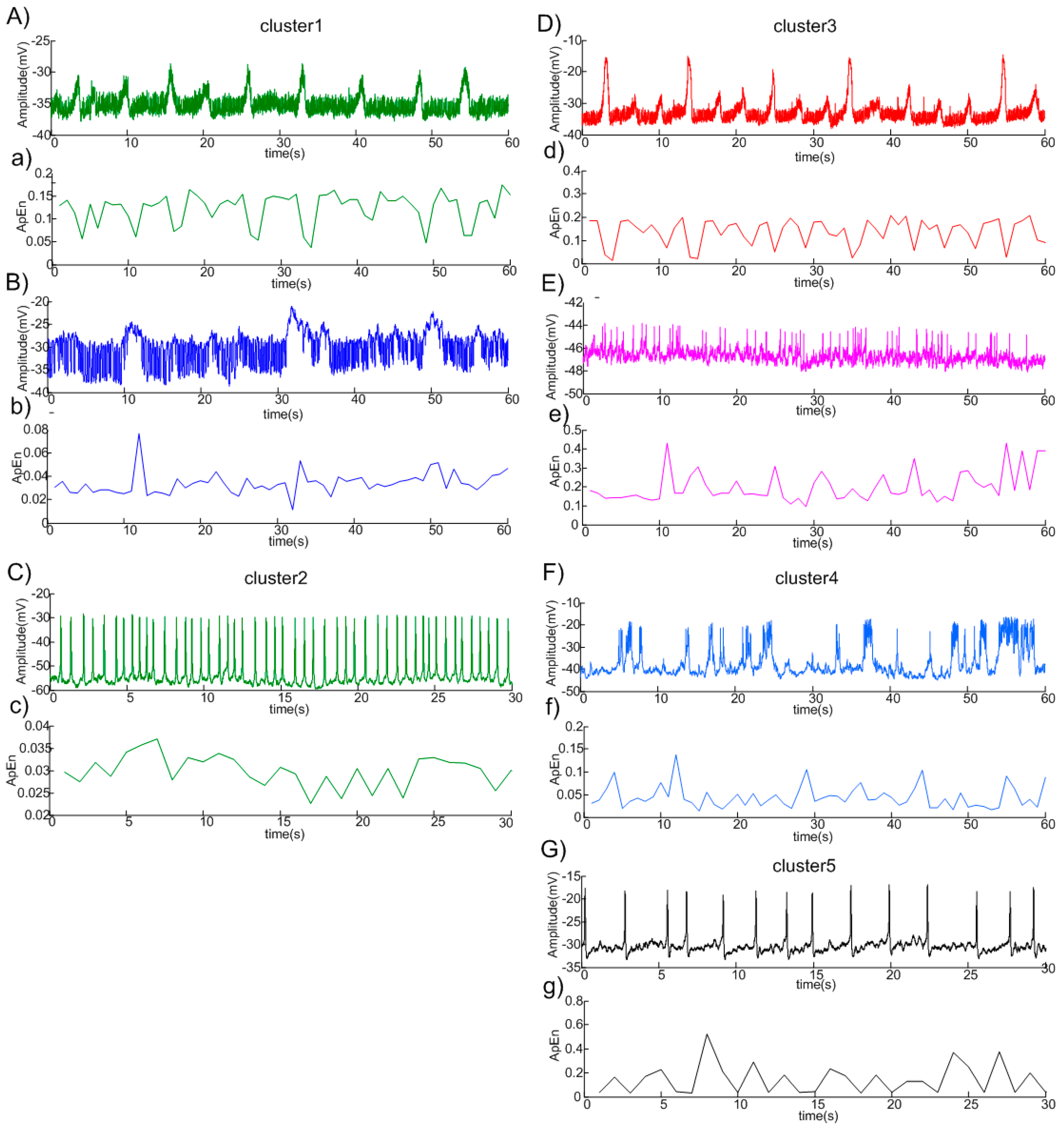
3.2. Clustering Results

We adopted 12 recordings of different neurons in SOG. As the oscillation status varied over time, we took three sections of each recording, each section lasted for 60 s, and obtained 36 types of waveforms as a result. The ApEn values of each oscillation were firstly obtained. From the tests of normality of 36 groups of ApEn data, it was found that the normality could not be well satisfied, with p values of 11 groups were > 0.05 and 25 groups were < 0.05. To test the difference between the ApEn distribution levels of 36 kinds of oscillations, we performed the Kruskal-Wallis instead of the ANOVA test to examine the difference between 36 groups. The p was < 0.01 (Table 1). What is more, the differences between the waveforms selected from one recording are statistically significant, while the waveform after stimulation by dopamine has no statistical significance with p > 0.01.
Table 1. Result of Kruskal-Wallis test of 12 groups of recordings.
No. of RecordingsNo. of OscillationsNo. of ApEn Values for every OscillationKruskal–Wallis Test
11/2/360p < 0.01
24/5/660p = 0.182
37/8/960p < 0.01
410/11/1260p < 0.01
513/14/1560p < 0.01
616/17/1860p < 0.01
719/20/2160p < 0.01
822/23/2460p < 0.01
925/26/2760p < 0.01
1028/29/3060p < 0.01
1131/32/3360p < 0.01
1234/35/3660p < 0.01
Total362160p < 0.01
The Kruskal-Wallis test of the total 36 selected sets of data shows that the total p is <0.01. The Kruskal–Wallis tests within the 3 sets of one recording show that the differences among each waveform selected from once recording were statistically significant, except that the waveforms recorded after being stimulated by dopamine have no statistically significant with p > 0.01.
Putting the ApEn of the 36 waveforms together, two ApEn oscillation patterns were simply displayed: one features low and fixed complexity while the other fluctuates severely. The indicators of ApEn in different neurons are different from each other, the oscillations in the same neuron also differ (Figure 2A,B). The MA and CVA were used as the variables to calculate the distances in the hierarchical clustering method.
Figure 2. Clustering results of 36 kinds of signals. (A) the MA of 36 kinds of signals; (B) the CVA of 36 kinds of signals; (C) the scatter diagram, taking the MA as abscissas and CVA as ordinates. The five different markers represent five different clusters; (D) the dendrogram by hierarchical clustering, wherein the dashed line shows the threshold of 0.15.
Entropy 17 06854 g002
The clustering result in Figure 2D shows the differences between the oscillations; a longer horizontal line signifies a longer distance .The coefficient of cophenet is 0.84. Combining clustering results with the spike patterns, we took 0.15 as the threshold of the between-class distance, and these oscillation patterns were divided into five categories. Figure 3A–G shows the clustering results and the corresponding original oscillations.
The first cluster has relatively low MA staying below 0.15 with CVA staying around 0.25. Figure 3A shows a mixed oscillation pattern, consisting of large amplitude waves with small amplitude waves in between. Figure 3B shows the activity of a neuron with a mixed pattern after being stimulated by dopamine (the next section will go into detail).
The second cluster had a discharge pattern with both low MA almost below 0.15 and CVA below 0.2, manifested as constant and regular signals with quasi-periodicity. Most oscillations belong to this pattern, and the peak values always stand between 10 and 20 mV. This is named the continuous spike pattern.
Figure 3. Five clusters of the original oscillation patterns and the corresponding ApEn values. The columns in A-L signify original oscillation sequences, while the corresponding a-1 below illustrate change sequences of ApEn values. Cluster 1 contains two oscillation patterns. Cluster 2 contains the continuous spike pattern. Cluster 3 contains two oscillation patterns, which were referred to as the mixed oscillation pattern and spikelet pattern respectively. Cluster 4 contains one oscillation pattern mixed with bursting oscillation and long-term excitability. Cluster 5 contains the sparse spike pattern.
Entropy 17 06854 g003
The third cluster featured with high MA (0.15–0.3) and CVA staying around 0.45. Two corresponding types of discharge were observed: the first is of mixed signals with lower MA, which is referred to as the mixed oscillation pattern; the second type which records continuous and dense signals with less and smaller spikelet rising on the oscillations is called the spikelet pattern. The spikelet pattern is composed of single wavelet amplitude which is generally less than 5 mV with duration of 100–500 ms.
The fourth cluster had a relatively low MA (0.05–0.15) and the CVA staying around 0.6. The number of oscillations belonging to this pattern ranks second. The corresponding discharge was mixed with bursting oscillation discharge and has long-term excitability during certain periods. The plateaus lasting from 1 to 10 s frequently emerges and the depolarization can reach −20 mV. This is what we called the bursting pattern, featuring long lasting depolarization discharge and stable spontaneous discharge.
The fifth cluster featured relatively low MA (0.05–0.15) and the high CVA staying around 0.8, which was quite high. The corresponding discharge signal was also consistent and regular, but compared with the second cluster, the frequency of action potentials was lower. This is sparse spike pattern.

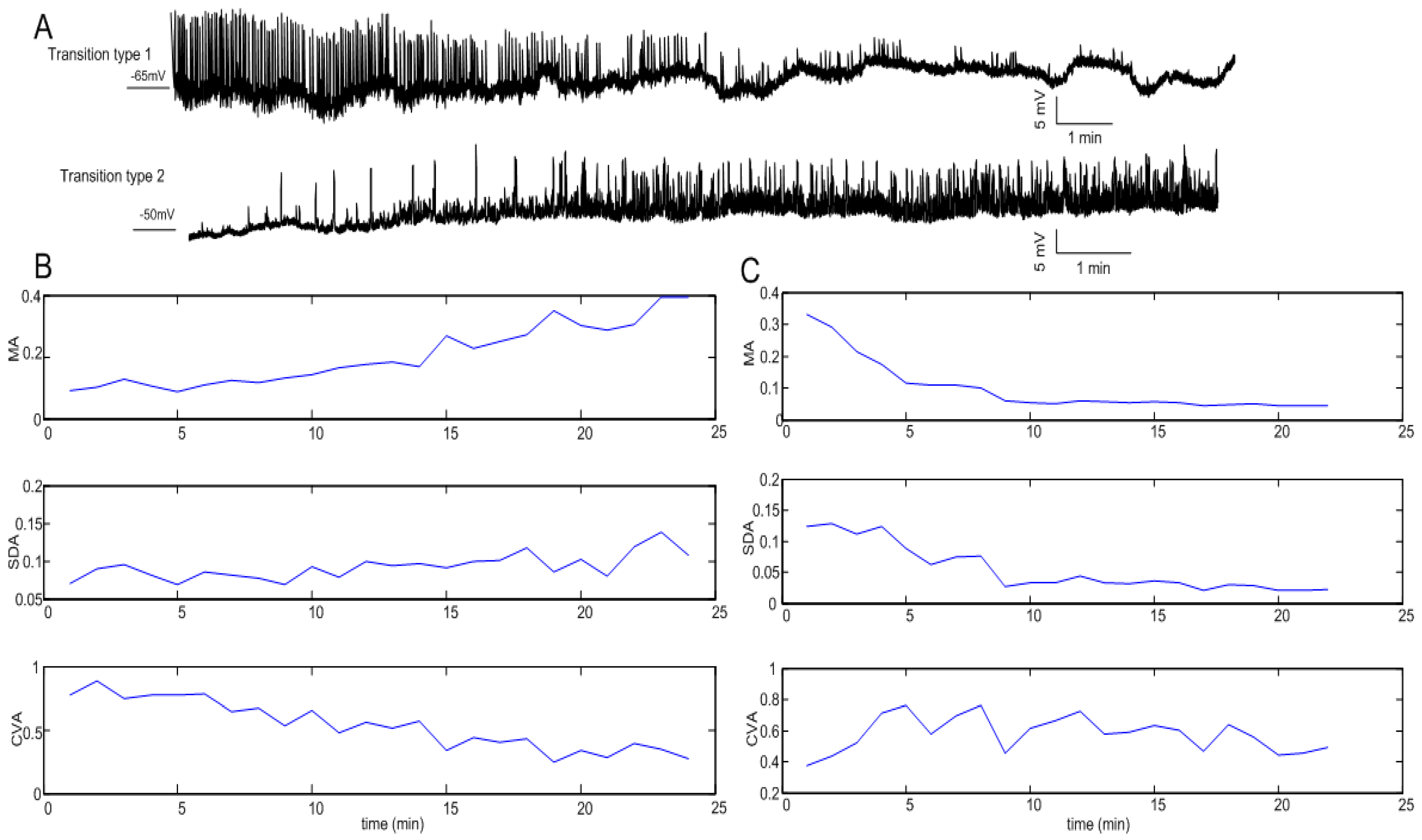
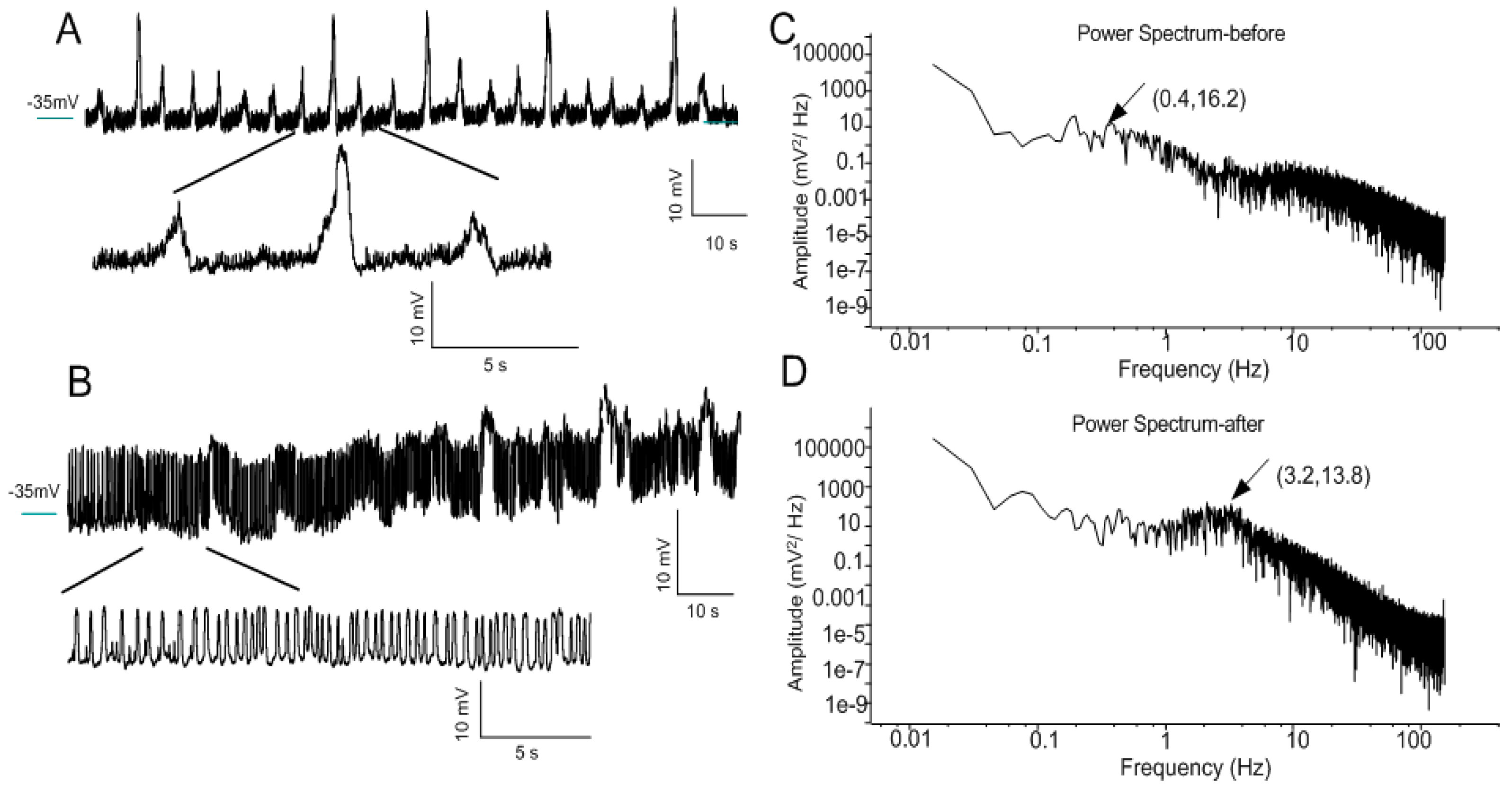
3.3. Transformation of Oscillation
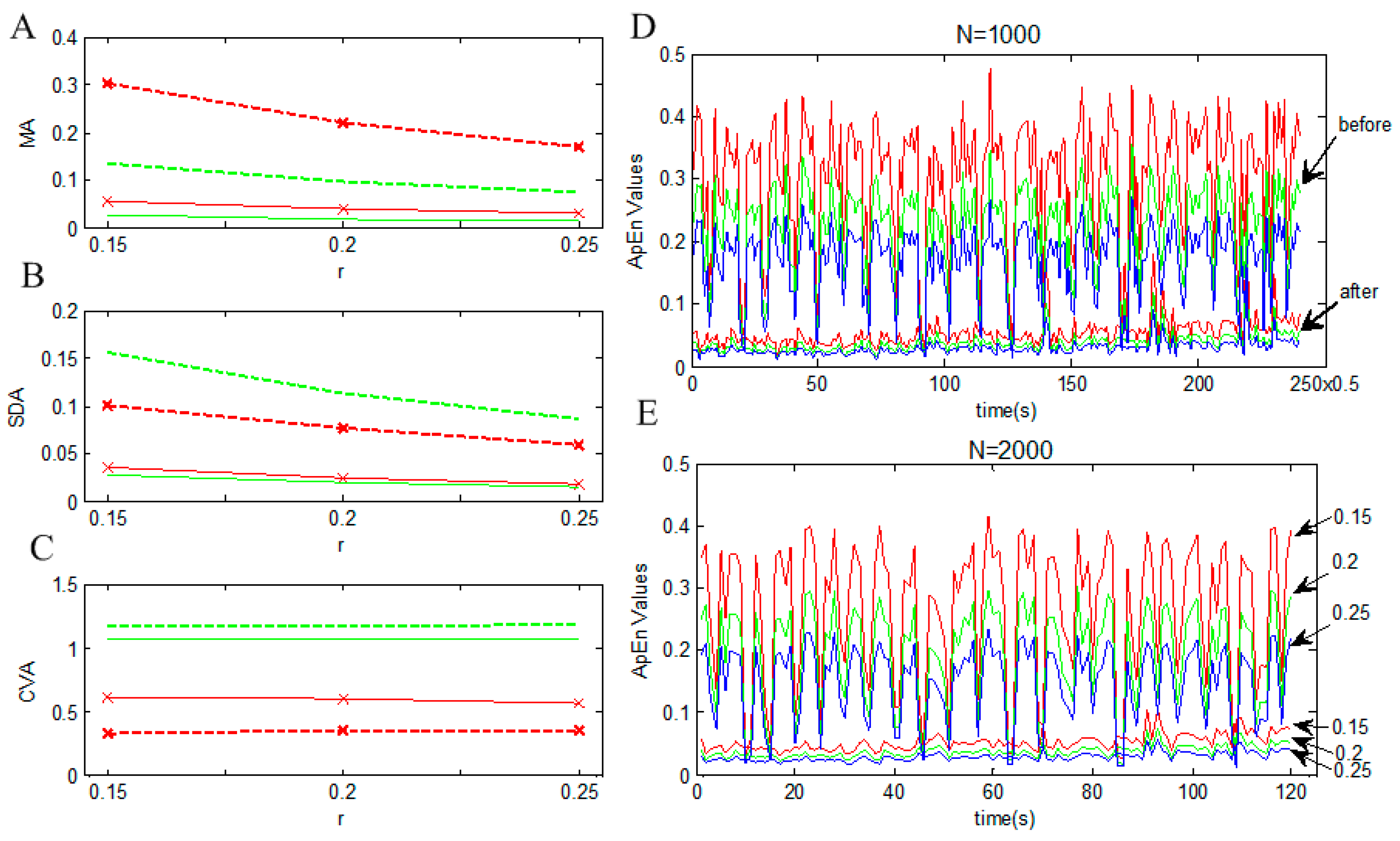
By adding the dopamine to the external solution, the embedded component of mixed electric signals would be disturbed and single continuous depolarized discharge emerges (Figure 4A,B). Distribution of power spectrum was calculated. Before the stimulation, the power spectrum of signals has no obvious peak values with most energy volume below 1 Hz (Figure 4C). After stimulation of dopamine, oscillation is featured with sine-like oscillation with amplitude of 10 mV (Figure 4B). As shown in Figure 4D, the proportion of 2–5 HZ component has an increase.
Figure 4. Changes of oscillation caused by dopamine. (A) oscillation signals of 2 min before stimulation by dopamine. There are at least two sorts of spike potentials. The average amplitude of large waves is about 20 mV. The small waves are about 8 mV which are formed by smaller waves with amplitudes of less than 4 mV; (B) oscillation signals of 2 min after stimulation by dopamine; (C) power spectrum of signals with most energy volume below 1 Hz before the stimulation. The abscissa and ordinate is Log-Log; (D) power spectrum of signals after the stimulation.
Entropy 17 06854 g004
Compared with the power spectrum results, the difference between the ApEn results of this alternation is more significant. The baseline of oscillation before stimulation is obvious higher (MA = 0.074) than that of oscillation after stimulation (MA = 0.015), regardless of changes of sample points or parameters in the calculation. Three statistical indicators of ApEn also show a significant difference (Table 2). The ApEn values after stimulation keep quite stable and relatively low while the ApEn values before stimulation fluctuate, which indicates a quasi-periodic change of probability for occurrence of new information (Figure 5D,E). Increasing sample points can reduce the MA while the SDA and CVA will increase. Increasing coefficient of r can reduce the MA and the SDA while CVA hardly changes.
Figure 5. ApEn results under different calculation conditions. Dashed lines indicate corresponding indicators of oscillation of 2 min before the simulation. Solid lines indicate corresponding indicators of oscillation of 2 min after the simulation. Red lines with * indicate samples of 1000. Green lines indicate samples of 2000. With the increase of ApEn threshold r from 0.15 to 0.25, the MA and the SDA have a decreasing trend; the corresponding gaps between the two oscillations become narrower. With the increase of sample point number N from 1000 to 2000, the MA decreases while the SDA and the CVA increase; the gaps of the MA and CVA between the two oscillations become narrower while the gap of the SDA becomes wider.
Entropy 17 06854 g005
Table 2. Values of the three statistical indicators of six ApEn parameters groups.
Sample Points(N)The Threshold Coefficient(r)MA-beforeMA-afterSDA-beforeSDA-afterCVA-beforeCVA-after
10000.150.3020.0570.1000.0350.3320.616
10000.20.2200.0400.0760.0240.3470.596
10000.250.1690.0310.0600.0180.3550.564
20000.150.1340.0260.1570.0281.1681.067
20000.20.0970.0190.1140.0201.1781.064
20000.250.0740.0150.0870.0161.1801.064
In fact, the simple sine-like oscillation status after the stimulation only lasted about 50 s with the ApEn values started to peak instead of remaining low. The complexity of the oscillation began to resume, indicating that the neuron ability of regulating oscillation also began to recover.

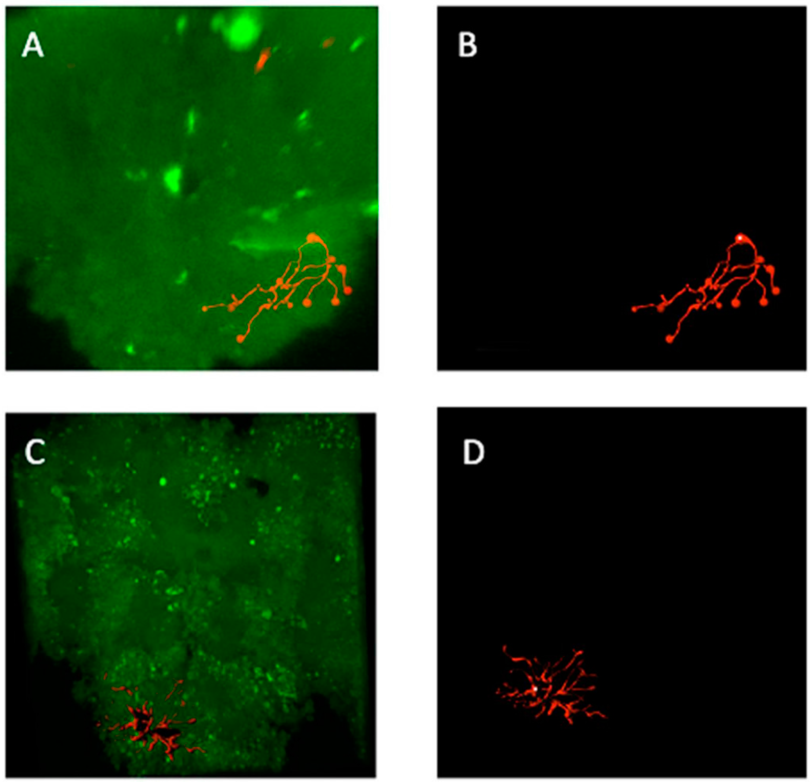
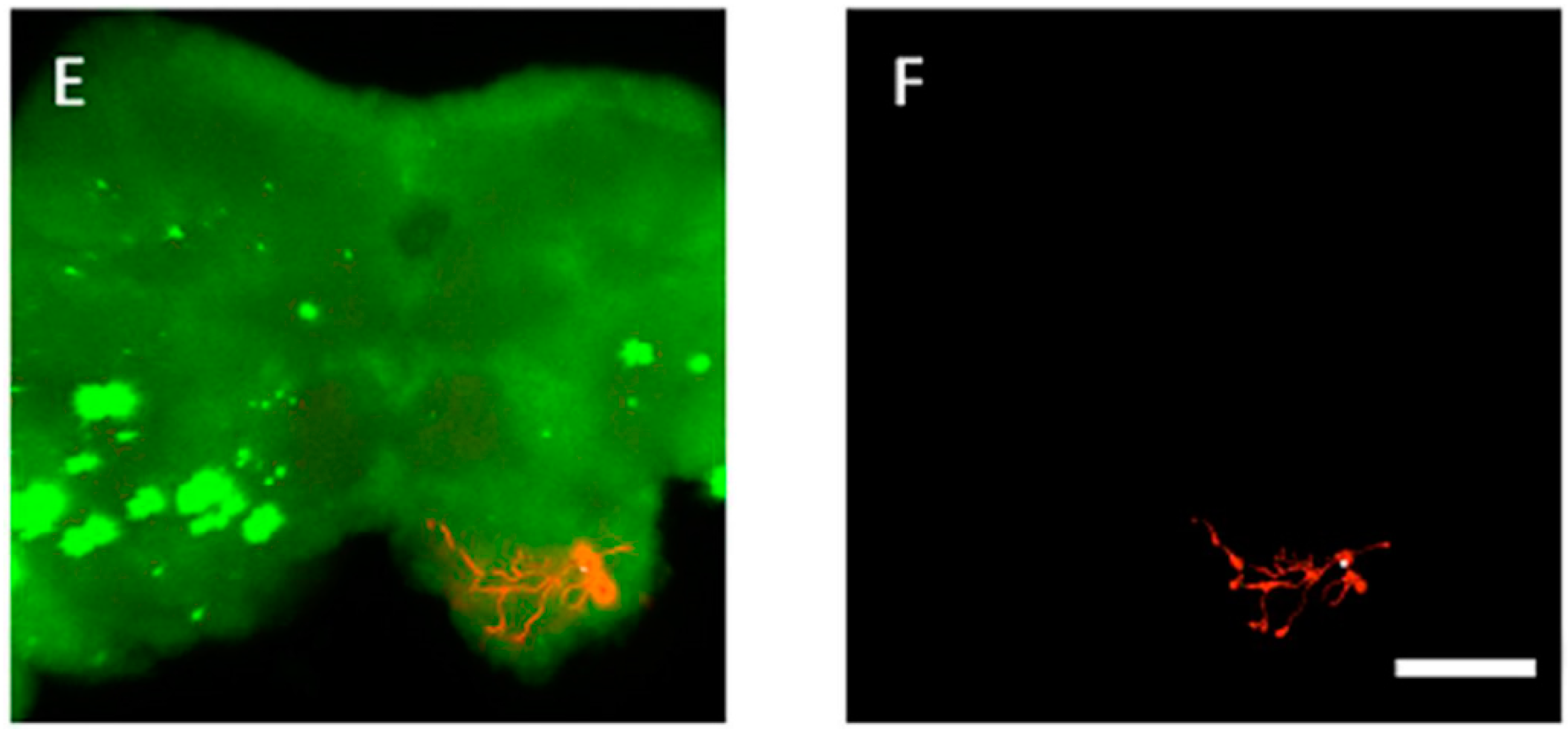
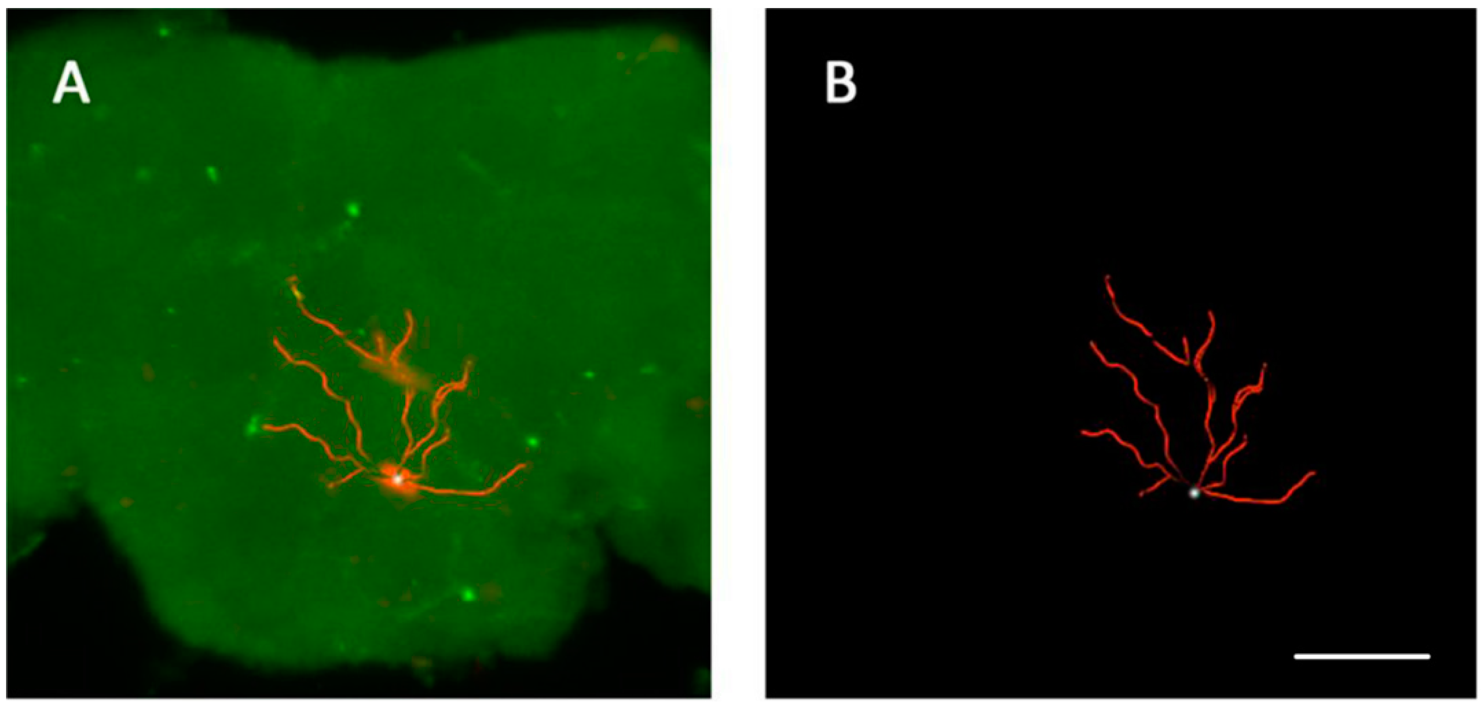
3.4. The Location of Neurons with Certain Pattern

The projection in SOG is very similar with local interneurons (LNs) in AL [36], with its trajectory area only located on the soma ipsilateral hemisphere of SOG (Figure 6). The biocytin staining and confocal imaging methods were according to what we described before [37]. Neurons’ morphology is visualized by imaris 8.0 (Bitplane). The filament toolbox is applied to highlight the axonal trace and trajectory. Electrophysiologically, spontaneous action potentials (SAPs) of LNs demonstrated a bursting pattern of sodium channel dependent spikes, and spikes no fewer than two were considered as a burst. SAPs of projection neurons demonstrated lower frequency with less and smaller spikelets rising on the oscillations. The bursting pattern is mainly in large neurons of the central portion of one side of SOG (Figure 7).The mixed oscillation pattern is located in the bottom of the central partial small neurons (Figure 6C).
Figure 6. The neurons with cell bodies located in the edge region of SOG. The scale is 80 μm. Soma and projection region of the neurons are in the same side of SOG, and the coverage of neurons does not exceed the SOG zone itself.
Entropy 17 06854 g006aEntropy 17 06854 g006b
Figure 7. The neurons with cell bodies located in the central region of SOG. The scale is 50 μm. The projection range exceeded SOG area.
Entropy 17 06854 g007

4. Discussion

4.1. ApEn of Neuron Oscillation

It is acknowledged that the oscillation of neurons consist of abundant information [6,38]. Because of the complexity of the background oscillations and other noises, detecting a specific oscillation like burst activity or spiking is a long-standing challenge in investigating the dynamics of neuronal activity [4,39]. Global measures, such as CV and AI, were mainly used in previous studies [40,41]. Some irregularity metrics are tested based on the ISI properties, such as the Fano Factor [42], shape parameters of the ISI distribution etc. [33,43]. However, such measures are usually not directly related to the information amount alternation, and mostly they are based on the interspike interval distribution. ApEn can represent the degree of irregularity as well as quantity of information of any oscillation whether spike emerges or not. Stable fluctuation of ApEn values indicates a quasi-periodic change of amount of new information in the neuron. The more complex and instable the oscillation status presents, the greater the ApEn values will be, vice versa. When the oscillation status changes, either from the dense spiking to sparse spiking or from spiking to bursts, the ApEn values will change consistently, it can conceal details as well as zoom the sudden changing point like the emergence of peaks.

4.1.1. Three Indicators

When making threshold of ApEn a smaller value, the evaluation of new information will be more rigorous, and thus the greater ApEn will be obtained and the complexity and irregularity of data will be considered stronger [18]. But in our method, the value of r is less important as is has little effect on CVA. Sample point greatly affects the final values of the three statistical indicators, particularly the SDA. We recommend that the sample point should be large and reasonable, and we unify with the number per unit time.
The MA indicates the regularity and stability of the oscillation as a whole. The SDA reflects the fluctuation of ApEn, thus it indicates the whole degree of depolarization. A higher CVA may manifest more patterns than the given oscillation includes. The CVA is a relative value, while SDA is an absolute value, which makes SDA not a good indicator to overall variation of the irregular nature. Large SDA values may not be generated by oscillation itself, because it is directly related to the number of ApEn results. Therefore, the MA and CVA were selected in the cluster analysis. And the sample points calculated of all oscillation groups should be strictly unified to reduce the classification error caused by ApEn computing.

4.1.2. Clustering of Different Patterns

Most of the existing classification methods define the category of an oscillation according to the parameters of a typical oscillation pattern [44,45], and it is unknown how many kinds of oscillation exist in the SOG. Therefore, instead of judging whether a particular one belongs to a current category, our aim is to find out how many patterns of oscillation exist, to distinguish different neurons in SOG and to even discover new oscillation types.
As an unsupervised learning approach, hierarchical clustering algorithm was utilized to classify oscillation patterns. Different from existing methods, we do not define the types of oscillation beforehand. If the MA and the CVA can represent features of oscillations, similarities should exist within the same type of oscillations after clustering, and they have been confirmed by the clustering results. The continuous spike pattern and bursting pattern are the dominated patterns. When both the MA and the CVA stand at a relative high value, it can be doubted that the neuron is a glial cell.
Compared to other clusters, the first cluster of results obtained seems not quite satisfying. As seen from Figure 3, A, a, B, and b, their ApEn distribution is different; the MA of (b) appeared lower and steadier in general, and the raw signal (B) is more regular compared to signal (A). It is difficult to differentiate the two types by using the method of clustering analysis because they have similar CVAs. The solutions can be used to improve the clustering method and increasing the computed oscillation types.

4.2. Oscillations in SOG Region

The neuronal discharge patterns are usually described by three principle patterns, namely, regular, irregular, and bursty [44]. Combining clustering results with the spike patterns, we showed that the discharge patterns in SOG can be classified by a relatively quantitative method and five categories can be more reasonable, including continuous spike pattern, mixed oscillation pattern, bursting pattern, and sparse spike pattern. In many cases, bursts and oscillations can be considered as distinct properties and are thus measured separately. However, bursts and oscillations often occur simultaneously or in similar contexts [29].
In the present study, it is found that the oscillation patterns of single neurons are always fixed but the oscillation states are interchangeable under certain conditions. Neuron with a mixed oscillation pattern in SOG can be excited by amine neurotransmitters while other oscillation types do not have obvious effect. The continuous electrical activity of neurons is deemed relevant to maintaining information of external stimulus [12,46]. Dopamine can lead a drop of ApEn values of the mixed oscillation. More detailed changes can be detected by the MA, SDA, and CVA. We speculate that neurons of the mixed oscillation pattern in the SOG region are the intermediate local neurons in the SOG, playing the role of exchanging information of external stimuli. They may pass the message to peripheral nerves and could be excitatory neurons meditated by amine neurotransmitters [1,47]. And for neurons of the bursting pattern, the projection range exceeded SOG area, acting as a subordinate projection neuron. Neurons with such oscillations are worth further study.

Acknowledgments

We would like to thank Ying Yan, Yuhao Huang for their help on electrophysiological experiment operations and Jiaming Ding for his help on the writing composition. We would also like to thank the anonymous reviewers whose comments have improved this paper. The funding was from the National Natural Science Foundation of China (No. 61263011), the frontier and key technology innovation project of Guangdong Province (No. 2014B010118003) and the Science and Technology Program of Guangdong Province (No. 2013B060500043).

Author Contributions

Tian Mei and Yi Zhou conceived and designed the experiments. Tian Mei and Jingda Qiao developed the methodology and operated the experiment. Tian Mei, Yi Zhou and Jingda Qiao conducted the computational analysis of the data. Huaiyu Gu, Ziyi Chen, Kuiying Gu and Xianghua Tian participated in the discussion and checked the results. Tian Mei and Yi Zhou wrote the paper. All authors have read and approved the final manuscript.

Conflicts of Interest

The authors declare no conflict of interest.

References

  1. Olsen, S.R.; Wilson, R.I. Cracking neural circuits in a tiny brain: New approaches for understanding the neural circuitry of drosophila. Trends Neurosci. 2008, 31, 512–520. [Google Scholar] [CrossRef] [PubMed]
  2. Muqit, M.M.K.; Feany, M.B. Opinion: Modelling neurodegenerative diseases in drosophila: A fruitful approach? Nat. Rev. Neurosci. 2002, 3, 237–243. [Google Scholar] [CrossRef] [PubMed]
  3. Feany, M.B.; Bender, W.W. A drosophila model of parkinson’s disease. Nature 2000, 404, 394–398. [Google Scholar] [CrossRef] [PubMed]
  4. Braun, H.A.; Schwabedal, J.; Dewald, M.; Finke, C.; Postnova, S.; Huber, M.T.; Wollweber, B.; Schneider, H.; Hirsch, M.C.; Voigt, K.; et al. Noise-induced precursors of tonic-to-bursting transitions in hypothalamic neurons and in a conductance-based model. Chaos 2011, 21. [Google Scholar] [CrossRef] [PubMed]
  5. Scott, K.; Brady, R., Jr.; Axel, R.; Morozov, P.; Rzhetsky, A.; Cravchik, A.; Zuker, C. A chemosensory gene family encoding candidate gustatory and olfactory receptors in drosophila. Cell 2001, 104, 661–673. [Google Scholar] [CrossRef]
  6. Ito, I.; Bazhenov, M.; Ong, R.C.-Y.; Raman, B.; Stopfer, M. Frequency transitions in odor-evoked neural oscillations. Neuron 2009, 64, 692–706. [Google Scholar] [CrossRef] [PubMed]
  7. Masse, N.Y.; Turner, G.C.; Jefferis, G.S.X.E. Olfactory information processing in drosophila. Curr. Biol. 2009, 19, R700–R713. [Google Scholar] [CrossRef] [PubMed]
  8. Martinez, D.; Montejo, N. A model of stimulus-specific neural assemblies in the insect antennal lobe. PLoS Comput. Biol. 2008, 4. [Google Scholar] [CrossRef] [PubMed]
  9. Yan, Y.; Xu, Y.; Deng, S.; Huang, N.; Yang, Y.; Qiu, J.; Liu, J.; Wang, X.; Yang, G.; Gu, H. A pair of identified giant visual projection neurons demonstrates rhythmic activities before eclosion. Neurosci. Lett. 2013, 550, 156–161. [Google Scholar] [CrossRef] [PubMed]
  10. Ran, D.; Cai, S.; Gu, H.; Wu, H. Di (2-ethylhexyl) phthalate modulates cholinergic mini-presynaptic transmission of projection neurons in drosophila antennal lobe. Food Chem. Toxicol. 2012, 50, 3291–3297. [Google Scholar] [CrossRef] [PubMed]
  11. Yang, Y.; Yan, Y.; Zou, X.; Zhang, C.; Zhang, H.; Xu, Y.; Wang, X.; Gu, H.; Yang, Z.; Janos, P. Static magnetic field modulates rhythmic activities of a cluster of large local interneurons in drosophila antennal lobe. J. Neurophysiol. 2011, 106, 2127–2135. [Google Scholar] [CrossRef] [PubMed]
  12. Tenney, J.R.; Fujiwara, H.; Horn, P.S.; Vannest, J.; Xiang, J.; Glauser, T.A.; Rose, D.F. Low- and high-frequency oscillations reveal distinct absence seizure networks. Ann. Neurol. 2014, 76, 558–567. [Google Scholar] [CrossRef] [PubMed]
  13. Flint, R.D.; Lindberg, E.W.; Slutzky, M.W.; Jordan, L.R.; Miller, L.E. Accurate decoding of reaching movements from field potentials in the absence of spikes. J. Neural Eng. 2012, 9. [Google Scholar] [CrossRef] [PubMed]
  14. Kirli, K.K.; Ermentrout, G.B.; Cho, R.Y. Computational study of nmda conductance and cortical oscillations in schizophrenia. Front. Comput. Neurosci. 2014, 8. [Google Scholar] [CrossRef] [PubMed]
  15. Orlandi, J.G.; Soriano, J.; Stetter, O.; Geisel, T.; Battaglia, D. Transfer entropy reconstruction and labeling of neuronal connections from simulated calcium imaging. PLoS ONE 2014, 9. [Google Scholar] [CrossRef] [PubMed] [Green Version]
  16. Wichmann, T.; Soares, J. Neuronal firing before and after burst discharges in the monkey basal ganglia is predictably patterned in the normal state and altered in parkinsonism. J. Neurophysiol. 2006, 95, 2120–2133. [Google Scholar] [CrossRef] [PubMed]
  17. Rinzel, J.; Huguet, G. Nonlinear dynamics of neuronal excitability, oscillations, and coincidence detection. Commun. Pur. Appl. Math. 2013, 66, 1464–1494. [Google Scholar] [CrossRef] [PubMed]
  18. Pincus, S. Approximate entropy as an irregularity measure for financial data. Economet. Rev. 2008, 27, 329–362. [Google Scholar] [CrossRef]
  19. Zhang, Z.; Chen, Z.; Zhou, Y.; Du, S.; Zhang, Y.; Mei, T.; Tian, X. Construction of rules for seizure prediction based on approximate entropy. Clin. Neurophysiol. 2014, 125, 1959–1966. [Google Scholar] [CrossRef] [PubMed]
  20. Burioka, N.; Cornelisson, G.; Halberg, F.; Kaplan, D.T.; Suyama, H.; Sako, T.; Shimizu, E.I. Approximate entropy of human respiratory movement during eye-closed waking and different sleep stages. Chest 2003, 123, 80–86. [Google Scholar] [CrossRef] [PubMed]
  21. Levy, W.J.; Pantin, E.; Mehta, S.; McGarvey, M. Hypothermia and the approximate entropy of the electroencepbalogram. Anesthesiology 2003, 98, 53–57. [Google Scholar] [CrossRef] [PubMed]
  22. Kalayci, T.; Ozdamar, O. Wavelet preprocessing for automated neural network detection of EEG spikes. IEEE Eng. Med. Biol. 1995, 14, 160–166. [Google Scholar] [CrossRef]
  23. Sanders, T.H.; Clements, M.A.; Wichmann, T. Parkinsonism-related features of neuronal discharge in primates. J. Neurophysiol. 2013, 110, 720–731. [Google Scholar] [CrossRef] [PubMed]
  24. Gu, H.; O’Dowd, D.K. Cholinergic synaptic transmission in adult drosophila kenyon cells in situ. J. Neurosci. 2006, 26, 265–272. [Google Scholar] [CrossRef] [PubMed]
  25. Pincus, S.M. Approximate entropy as a measure of system complexity. Proc. Natl. Acad. Sci. USA 1991, 88, 2297–2301. [Google Scholar] [CrossRef] [PubMed]
  26. Holzinger, A.; Jurisica, I. Knowledge Discovery and Data Mining in Biomedical Informatics: The Future is in Integrative, Interactive Machine Learning Solutions; Springer: Berlin/Heidelberg, Germany, 2014; pp. 1–18. [Google Scholar]
  27. Mayer, C.C.; Bachler, M.; Hoertenhuber, M.; Stocker, C.; Holzinger, A.; Wassertheurer, S. Selection of entropy-measure parameters for knowledge discovery in heart rate variability data. BMC Bioinform. 2014, 15. [Google Scholar] [CrossRef] [PubMed]
  28. Perkel, D.H.; Gerstein, G.L.; Moore, G.P. Neuronal spike trains and stochastic point processes. I. The single spike train. Biophys. J. 1967, 7, 391–418. [Google Scholar] [CrossRef]
  29. Markus, B.; Schiemann, J.; Roeper, J.; Schneider, G. Measuring burstiness and regularity in oscillatory spike trains. J. Neurosci. Methods 2011, 201, 426–437. [Google Scholar]
  30. Witham, C.L.; Baker, S.N. Information theoretic analysis of proprioceptive encoding during finger flexion in the monkey sensorimotor system. J. Neurophysiol. 2015, 113, 295–306. [Google Scholar] [CrossRef] [PubMed]
  31. Yu, Y.; Tang, H.; Han, X.; Bi, Q. Bursting mechanism in a time-delayed oscillator with slowly varying external forcing. Commun. Nonlinear Sci. 2014, 19, 1175–1184. [Google Scholar] [CrossRef]
  32. Manis, G. Fast computation of approximate entropy. Comput. Methods Programs Biomed. 2008, 91, 48–54. [Google Scholar] [CrossRef] [PubMed]
  33. Davies, R.M.; Gerstein, G.L.; Baker, S.N. Measurement of time-dependent changes in the irregularity of neural spiking. J. Neurophysiol. 2006, 96, 906–918. [Google Scholar] [CrossRef] [PubMed]
  34. Meyer, A.; Galizia, C.G.; Nawrot, M.P. Local interneurons and projection neurons in the antennal lobe from a spiking point of view. J. Neurophysiol. 2013, 110, 2465–2474. [Google Scholar] [CrossRef] [PubMed]
  35. Wild, J.; Prekopcsak, Z.; Sieger, T.; Novak, D.; Jech, R. Computational neuroscience: Performance comparison of extracellular spike sorting algorithms for single-channel recordings. J. Neurosci. Methods 2012, 203, 369–376. [Google Scholar] [CrossRef] [PubMed]
  36. Huang, N.; Yan, Y.; Xu, Y.; Jin, Y.; Lei, J.; Zou, X.; Ran, D.; Zhang, H.; Luan, S.; Gu, H. Alumina nanoparticles alter rhythmic activities of local interneurons in the antennal lobe of drosophila. Nanotoxicology 2013, 7, 212–220. [Google Scholar] [CrossRef] [PubMed]
  37. Qiao, J.; Zou, X.; Lai, D.; Yan, Y.; Wang, Q.; Li, W.; Deng, S.; Xu, H.; Gu, H. Azadirachtin blocks the calcium channel and modulates the cholinergic miniature synaptic current in the central nervous system of drosophila. Pest Manag. Sci. 2014, 70, 1041–1047. [Google Scholar] [CrossRef] [PubMed]
  38. Pita-Almenar, J.D.; Yu, D.; Lu, H.-C.; Beierlein, M. Mechanisms underlying desynchronization of cholinergic-evoked thalamic network activity. J. Neurosci. 2014, 34, 14463–14474. [Google Scholar] [CrossRef] [PubMed]
  39. Chen, L.; Deng, Y.; Luo, W.; Wang, Z.; Zeng, S. Detection of bursts in neuronal spike trains by the mean inter-spike interval method. Prog. Nat. Sci. 2009, 19, 229–235. [Google Scholar] [CrossRef]
  40. Holt, G.R.; Softky, W.R.; Koch, C.; Douglas, R.J. Comparison of discharge variability in vitro and in vivo in cat visual cortex neurons. J. Neurophysiol. 1996, 75, 1806–1814. [Google Scholar] [PubMed]
  41. Shinomoto, S.; Kim, H.; Shimokawa, T.; Matsuno, N.; Funahashi, S.; Shima, K.; Fujita, I.; Tamura, H.; Doi, T.; Kawano, K.; et al. Relating neuronal firing patterns to functional differentiation of cerebral cortex. PLoS Comput. Biol. 2009, 5. [Google Scholar] [CrossRef] [PubMed]
  42. Christodoulou, C.; Bugmann, G. Coefficient of variation vs. Mean interspike interval curves: What do they tell us about the brain? Neurocomputing 2001, 38, 1141–1149. [Google Scholar] [CrossRef]
  43. Maimon, G.; Assad, J.A. Beyond poisson: Increased spike-time regularity across primate parietal cortex. Neuron 2009, 62, 426–440. [Google Scholar] [CrossRef] [PubMed]
  44. Kumbhare, D.; Baron, M.S. A novel tri-component scheme for classifying neuronal discharge patterns. J. Neurosci. Methods 2015, 239, 148–161. [Google Scholar] [CrossRef] [PubMed]
  45. Taube, J.S. Interspike interval analyses reveal irregular firing patterns at short, but not long, intervals in rat head direction cells. J. Neurophysiol. 2010, 104, 1635–1648. [Google Scholar] [CrossRef] [PubMed]
  46. Machens, C.K.; Romo, R.; Brody, C.D. Flexible Control of Mutual Inhibition: A Neural Model of Two-Interval Discrimination. Science 2005, 307, 1121–1124. [Google Scholar] [CrossRef] [PubMed]
  47. Tanaka, N.K.; Stopfer, M.; Ito, K. Odor-evoked neural oscillations in drosophila are mediated by widely branching interneurons. J. Neurosci. 2009, 29, 8595–8603. [Google Scholar] [CrossRef] [PubMed]

