
Setting Diverging Colors for a Large-Scale Hypsometric Lunar Map Based on Entropy

Abstract
:1. Introduction
2. Data Source and Method
2.1. CE2 Lunar DEM Data
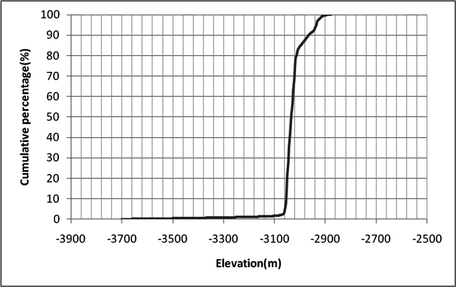
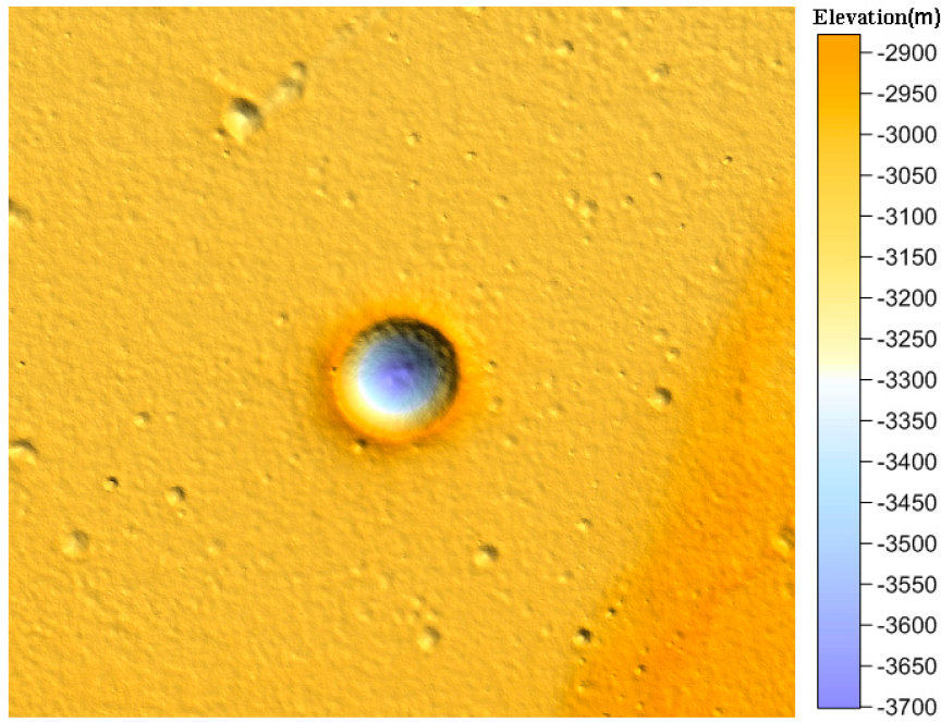
2.1.1. Data Characteristics
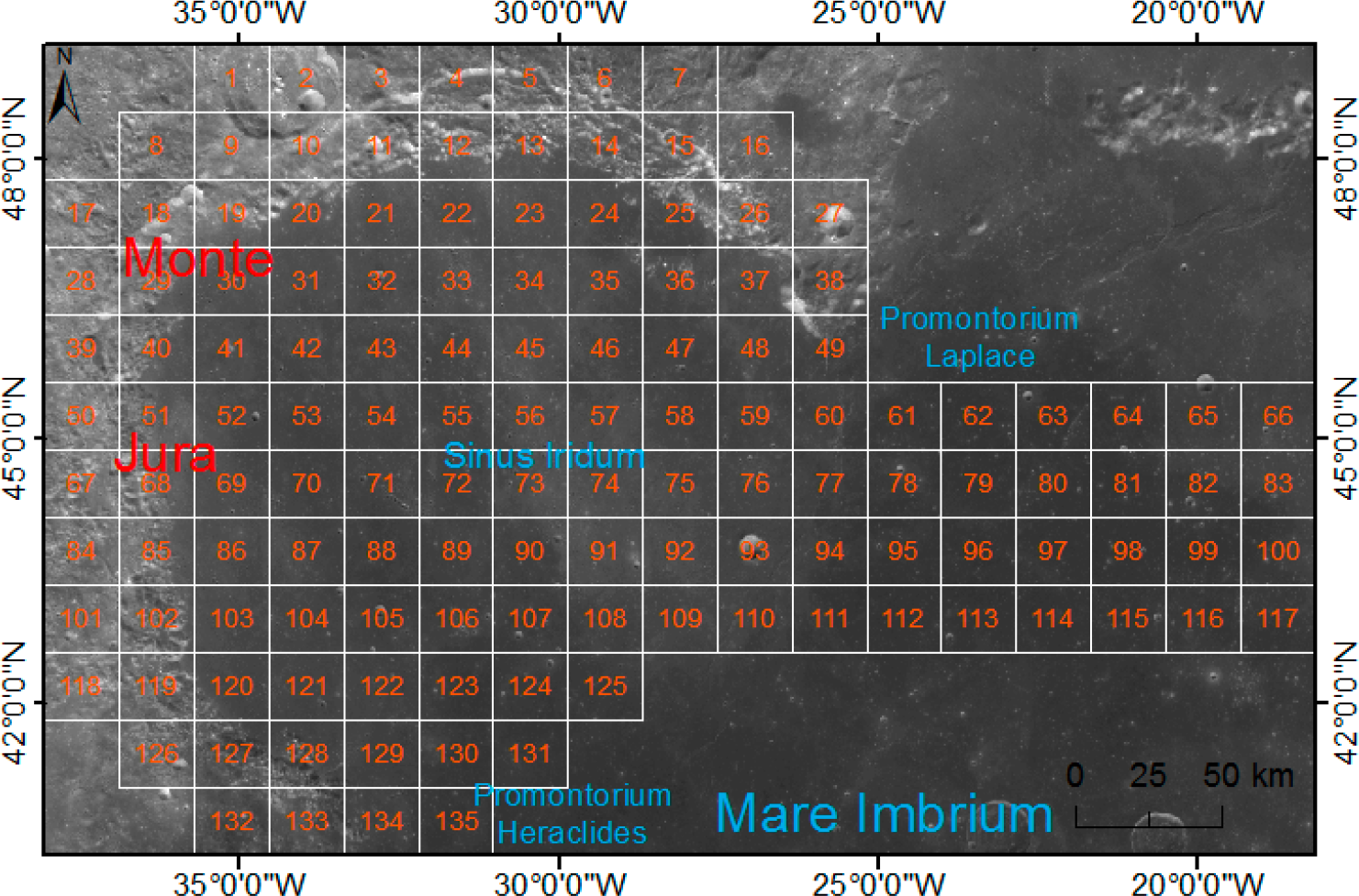
2.1.2. Mapping Areas
2.2. Diverging Color Setting Method
2.2.1. Problems in Color Setting
2.2.2. Diverging-Colors Setting Rules Based on Entropy
2.2.3. Apply the Rules in the Color Setting of a Lunar Hypsometric Map

| 1: | // RGB parameters |
| 2: | C(r,g,b); |
| 3: | // CIE-XYZ parameters |
| 4: | C(x,y,z); |
| 5: | // CIE-LAB parameters; |
| 6: | C(l,a,b); |
| 7: | double Xn = 96.4221; |
| 8: | double Yn = 100; |
| 9: | double Zn = 82.5221; |
| 10: | // RGB to CIE-XYZ parameters |
| 11: | double rxf = 0.17697; |
| 12: | double xr = 0.49; |
| 13: | double xg = 0.31; |
| 14: | double xb = 0.2; |
| 15: | double yr = 0.17697; |
| 16: | double yg = 0.81240; |
| 17: | double yb = 0.01063; |
| 18: | double zr = 0; |
| 19: | double zg = 0.01; |
| 20: | double zb = 0.99; |
| 21: | double rx = 2.36461; |
| 22: | double ry = −0.89654; |
| 23: | double rz = −0.46807; |
| 24: | double gx = −0.51517; |
| 25: | double gy = 1.42641; |
| 26: | double gz = 0.08876; |
| 27: | double bx = 0.0052; |
| 28: | double by = −0.01441; |
| 29: | double bz = 1.0092; |
| 30: | // RGB to CIE-XYZ |
| 31: | x = (xr × r + xg × g + xb × b)/rxf; |
| 32: | y = (yr × r + yg × g + yb × b)/rxf; |
| 33: | z = (zr × r+zg × g+zb × b)/rxf; |
| 34: | // DivideN(double dn) |
| 35: | if (dn > Math.pow(6.0/29.0, 3)) then DivideN(dn) = Math.pow(dn,1.0/3); |
| 36: | else DivideN(dn) = 1.0/3.0 × 29.0/6.0 × 29.0/6.0 × dn + 16.0/116.0; |
| 37 | // CIE-XYZ to CIE-LAB |
| 38: | l = DivideN(y/Yn) × 116 − 16; |
| 39: | a = 500 × (DivideN(x/Xn) – DivideN(y/Yn)); |
| 40: | b = 200 × (DivideN(y/Yn) – DivideN(z/Zn)); |
| 41: | Return C(l,a,b) |
| 1: | // Color parameters |
| 2: | Cmin(l1,a1,b1); |
| 3: | Cmax(l2,a2,b2); |
| 4: | Ci(li,ai,bi); |
| 5: | // Cdis(Cmin,Cmax) |
| 6: | Cdis(Cmin, Cmax) = Math.sqrt(Math.pow((l1 − l2), 2) + Math.pow((a1 − a2), 2) + Math.pow((b1 − b2), 2)); |
| 7: | // Calculate Ci |
| 8: | t = Cdis(Cmin,Ci)/Cdis(Ci,Cmax); |
| 9: | li = (l1 + t × l2)/(1 + t); |
| 10: | ai = (a1 + t × a2)/(1 + t); |
| 11: | bi = (b1 + t × b2)/(1 + t); |
| 12: | Return Ci(li,ai,bi) |
| 1: | // CIE-LAB to CIE-XYZ |
| 2: | // Parameters are the same as Algorithm 1. |
| 3: | double fy = (l + 16.0)/116.0; |
| 4: | if (fy > 6.0/29) then y = Yn × Math.pow(fy, 3); |
| 5: | else y = (fy − 16.0/116.0) × 3 × 6.0/29.0 × 6.0/29.0 × Yn; |
| 6: | double fx = fy + a/500; |
| 7: | if (fx > 6.0/29) then x = Xn × Math.pow(fx, 3); |
| 8: | else x = (fx − 16.0/116.0) × 3 × 6.0/29.0 × 6.0/29.0 × Xn; |
| 9: | double fz = fy − b/200; |
| 10: | if (fz > 6.0/29) then z = Zn × Math.pow(fz, 3); |
| 11: | else z = (fz − 16.0/116.0) × 3 × 6.0/29.0 × 6.0/29.0 × Zn; |
| 12: | // CIE-XYZ to RGB |
| 13: | r = (rx × x + ry × y + rz × z) × rxf; |
| 14: | g = (gx × x + gy × y + gz × z) × rxf; |
| 15: | b = (bx × x + by × y + bz × z) × rxf; |
| 16: | Return C(r,g,b) |
3. Results and Discussion
4. Conclusions
Acknowledgments
Author Contributions
Conflicts of Interest
References
- Shannon, C.E. A Mathematical Theory of Communication. Bell Syst. Tech. J 1948, 27, 379–423. [Google Scholar]
- Batty, M. Spatial Entropy. Geogr. Anal. 1974, 6, 1–31. [Google Scholar]
- Pászto, V.; Tuček, P.; Voženílek, V. On Spatial Entropy in Geographical Data, Proceedings of the GIS Ostrava, Ostrava, Czech Republic, 25–28 January 2009.
- Batty, M. Space, Scale and Scaling in Entropy Maximizing. Geogr. Anal. 2010, 42, 395–421. [Google Scholar]
- Sofia, G.; Tarolli, P.; Cazorzi, F.; Dalla Fontana, G. An Objective Approach for Feature Extraction: Distribution Analysis and Statistical Descriptors for Scale Choice and Channel Network Identification. Hydrol. Earth Syst. Sci. 2011, 15, 1387–1402. [Google Scholar]
- Sofia, G.; Dalla Fontana, G.; Tarolli, P. High-Resolution Topography and Anthropogenic Feature Extraction: Testing Geomorphometric Parameters in Floodplains. Hydrol. Process. 2014, 28, 2046–2061. [Google Scholar]
- Batty, M. Entropy in Spatial Aggregation. Geogr. Anal. 1976, 8, 1–21. [Google Scholar]
- Ruiz, M.; López, F.; Páez, A. Comparison of Thematic Maps Using Symbolic Entropy. Int. J. Geogr. Inf. Sci. 2012, 26, 413–439. [Google Scholar]
- Li, K.; Chen, J.; Tarolli, P.; Sofia, G.; Feng, Z.; Li, J. Geomorphometric Multi-Scale Analysis for the Automatic Detection of Linear Structures on the Lunar Surface. Earth Sci. Front. 2014, 21, 212–222. [Google Scholar]
- Bowker, D.E.; Hughes, J.K. Lunar Orbiter Photographic Atlas of the Moon; NASA Special Publication: Washington, DC, USA, 1971. [Google Scholar]
- Tiernan, M.; Roth, L.; Thompson, T.W.; Elachi, C.; Brown, W.E., Jr. Lunar Cartography with the Apollo 17 Alse Radar Imagery. The Moon. 1976, 15, 155–163. [Google Scholar]
- Kirk, R.L.; Archinal, B.A.; Gaddis, L.R.; Rosiek, M.R. Lunar Cartography: Progress in the 2000s and Prospects for the 2010s, International Archives of the Photogrammetry, Remote Sensing and Spatial Information Sciences, Volume XXXIX-B4, Proceedings of XXII ISPRS Congress, Melbourne, Australia, 25 August–1 September 2012.
- Bussey, B.; Spudis, P. The Clementine Atlas of the Moon; Cambridge University Press: Cambridge, UK, 2004. [Google Scholar]
- Araki, H.; Tazawa, S.; Noda, H.; Ishihara, Y.; Goossens, S.; Sasaki, S.; Kawano, N.; Kamiya, I.; Otake, H.; Oberst, J.; Shum, C. Lunar Global Shape and Polar Topography Derived from Kaguya-LALT Laser Altimetry. Science 2009, 323, 897–900. [Google Scholar]
- Li, C.L.; Liu, J.J.; Ren, X.; Mou, L.L.; Zou, Y.L.; Zhang, H.B.; Lü, C.; Liu, J.Z.; Zuo, W.; Su, Y.; et al. The Global Image of the Moon by the Chang’E-1: Data Processing and Lunar Cartography. Sci. China Earth Sci. 2010, 5(3), 1091–1102. [Google Scholar]
- Mu, L.L.; Li, C.L.; Liu, J.J.; Ren, X.; Zou, X.D. A New Mapping Method for the Moon with the Chang’E-1 Data. Proceedings of the 26th International Cartographic Conference, Dresden, Germany, 25–30 August 2013.


| Technical parameter | Content | |
|---|---|---|
| Spectrum range | 450 ~ 520 nm | |
| Quantization level | 8 bit | |
| MTF | ≥ 0.2 (considering the influence of speed altitude ratio adjustment) | |
| S/N (ρ = 0.2,θ = 60°) | ≥ 100 | |
| Gain | 3 selections (G = 0.7, 1.0, 2.0) | |
| Width of the image | 43 km (@ 100 km orbit), 9.2 km (@ 15 km orbit) | |
| Base to height ratio | ≥ 0.45 | |
| Pixel resolution | Better than 10 m | |
| Optical system factor | CCD Stereo camera focal length | 144.3 mm |
| Relative aperture | F/9 | |
| Integral number | 5 selections (16, 32, 48, 64 and 96) | |
| Stereo angle | Front view +8°, back view −17.2° | |
| CCD detective unit | Pixel number | 6144 |
| Pixel size | 10.1 μm × 10.1 μm | |
© 2015 by the authors; licensee MDPI, Basel, Switzerland This article is an open access article distributed under the terms and conditions of the Creative Commons Attribution license (http://creativecommons.org/licenses/by/4.0/).
Share and Cite
Zeng, X.; Mu, L.; Liu, J.; Yang, Y. Setting Diverging Colors for a Large-Scale Hypsometric Lunar Map Based on Entropy. Entropy 2015, 17, 5133-5144. https://doi.org/10.3390/e17075133
Zeng X, Mu L, Liu J, Yang Y. Setting Diverging Colors for a Large-Scale Hypsometric Lunar Map Based on Entropy. Entropy. 2015; 17(7):5133-5144. https://doi.org/10.3390/e17075133
Chicago/Turabian StyleZeng, Xingguo, Lingli Mu, Jianjun Liu, and Yiman Yang. 2015. "Setting Diverging Colors for a Large-Scale Hypsometric Lunar Map Based on Entropy" Entropy 17, no. 7: 5133-5144. https://doi.org/10.3390/e17075133
APA StyleZeng, X., Mu, L., Liu, J., & Yang, Y. (2015). Setting Diverging Colors for a Large-Scale Hypsometric Lunar Map Based on Entropy. Entropy, 17(7), 5133-5144. https://doi.org/10.3390/e17075133