Article

Entropy-Complexity Characterization of Brain Development in Chickens

by
Fernando Montani
1,2,* and
Osvaldo A Rosso
3,4
1
IFLYSIB, CONICET & Universidad Nacional de La Plata, La Plata, Argentina
2
Departamento de Física, Facultad de Ciencias Exactas, UNLP Calle 49 y 115. C.C. 67 (1900), La Plata, Argentina
3
Instituto de Física Universidade Federal de Alagoas (UFAL). BR 104 Norte km 97, 57072-970 Maceió, Alagoas, Brazil
4
Instituto Tecnológico Buenos Aires (ITBA), Av Eduardo Madero 399, C1106ACD Ciudad Autónoma de Buenos Aires, Argentina
*
Author to whom correspondence should be addressed.
Entropy 2014, 16(8), 4677-4692; https://doi.org/10.3390/e16084677
Submission received: 21 July 2014 / Accepted: 20 August 2014 / Published: 21 August 2014
(This article belongs to the Special Issue Entropy and Electroencephalography)

Abstract

:
Electroencephalography (EEG) reflects the electrical activity of the brain, which can be considered chaotic and ruled by a nonlinear dynamics. Chickens exhibit a protracted period of maturation, and this temporal separation of the synapse formation and maturation phases is analogous to human neural development, though the changes in chickens occur in weeks compared to years in humans. The development of synaptic networks in the chicken brain can be regarded as occurring in two broadly defined phases. We specifically describe the chicken brain development phases in the causality entropy-complexity plane H × C, showing that the complexity of the electrical activity can be characterized by estimating the intrinsic correlational structure of the EEG signal. This allows us to identify the dynamics of the developing chicken brain within the zone of a chaotic dissipative behavior in the plane H × C.
PACS classifications: 02.50.-r; 05.45. Tp;87.19.La

1. Introduction

The brain can be thought as a complex system, and the dynamical features of neural population activity emerge from the interactions of the neuro-anatomical networks. Mental states would emerge therefore from the interaction between multiple physical and functional levels. The nature of the relationship between the mind and the brain is far from understood. We may tend to think of the optimal brain development of a human, or a mouse, or a chicken, as something which is clearly limited by genes. However, if chickens or rats are provided with a stimulating environment, cognitive performances can be slightly improved as generations pass. On the contrary, if environmental stimuli and food supplies are discontinued, the brain inter-connectivity does not grow further. Thus, the conditions surrounding the organism could define how the neural system would evolve.
Developing theoretical tools that could provide new insights to study how mind/brain mechanisms evolve would crucially change our understanding of cognitive processes. In this paper, we show that recent advances in complex systems can provide crucial new insights into this problem. Electroencephalography (EEG) reflects the brains electrical activity, such as postsynaptic potentials, and functional magnetic resonance imaging (fMRI) detects blood flow, motion and equilibrium under the action of external forces. Importantly, EEGs contain information about the architecture of the neural networks in the brain on several scales. The detection of anomalies in EEG signals can be a biomarker for developmental cognitive disorders.
Bandt and Pompe [1] have proposed a robust approach to time series analysis on the basis of counting ordinal patterns by introducing the concept of permutation entropy for quantifying the complexity of a system behind a time series. Thus, the ordinal structures of the time series instead of the values themselves are considered taking into account the time causality of the signal [2]. This methodology has been applied for investigating EEG and FMRi signals [314]. The complexity of the brain would represent the amount of “information” contained in the organism, in the sense that it quantifies the dynamical features of the temporal pattern due to functional interactions produced by a structural network. Complexity captures the degree to which a neural system integrates specialized information, and in particular, MPRstatistical complexity can distinguish time series generated by stochastic and chaotic systems [15,16]. This statistical complexity measure can also detect and quantify noise induced order [15,16].
In this paper, we characterize EEG signals of chicken, from the time the birds have weekly measures until six weeks posthatch. We considered that in this period, the chickens reach their neurological maturity. We analyze the EEG time series corresponding to the first six weeks of life and perform a quantitative analysis of the brain maturation changes. By estimating Shannon entropy, MPR statistical complexity and the Fisher information measure [1719] of the EEGs signals, we show that it is possible to quantify brain development. Thus, using information theory-based quantifiers as biomarkers of chicken brain allows us to characterize the underline the dynamics of EEG time series, identifying the different stages of bird brain maturation. Our results show that synapse formation in the chicken brain occurs in the first stage between the first and the third week, where the system, instead of developing into a more complex state, moves to lower values, producing its entropic reduction, where it reaches a more ordered state (in agreement with [2022]). Once the chickens are between the third and sixth week, meeting the needs of the highly energetic, demanding and sensitive neuronal cells (helped with the proper conditions surrounding the organisms), it is said that they reach the “maturation period”. We show that during this second stage, the brain develops into a more complex state, but also, at the same time, producing its entropic deterioration as cells become older. Importantly, our analysis of the causality entropy-complexity plane H × C allows us to identify the localization of the developing chicken brain dynamics within the zone of a chaotic dissipative behavior in this plane.

2. Methodology

2.1. Experimental Methods

Twenty four chickens (Gallus domesticus) reared from hatching were the subjects in this experiment. All birds had free access to food and water throughout the experiment. The birds were reared initially in incubation boxes and then transferred to holding cages maintained at a constant temperature (21 °C) with a 12:12 h light:dark cycle. Continuous EEG recordings (0.1–100 Hz with a 50-Hz notch filter) were made using small (6 mm) gold cup electrodes attached to the scalp with collodion glue and filled with electrode gel. The signal was sampled at a rate of 128 Hz, passed through amplifiers and stored directly on a computer. The total length of each record is 16, 368 data. Data acquisition was controlled by Strawberry Tree software. Four electrodes were placed over the left and right frontal (LF and RF) and the left and right posterior (LP and RP) areas of the scalp, with an additional reference electrode placed at the back of the head. EEG recording was taken at Day 7 posthatch and then each week for six weeks. For additional details of the acquisition protocol, see [23]. The recorded EEG signals are nonstationary, and they also present artifacts, due to saccadic eye movements [23].
In order to avoid these problems and to facilitate a subsequent quantitative analysis, each signal was pre-processed using a methodology based on orthogonal discrete wavelet transform (see [24] for procedure details) and summarized as follow: (1) The discrete orthogonal wavelet transform of the signal is obtained considering Jmax = −10 wavelet resolution levels with a spline cubic mother wavelet. (2) After that, a cleaning and stationary signal is obtained by reconstruction (inverse wavelet transform) using the resolution wavelet levels corresponding to the frequency range 0.5–32.0 Hz. (3) The wavelet frequency bands at which the saccadic movement frequency appear, as well as their time localization were identified. The corresponding wavelet coefficients were reduced so that they present a contribution below the noise-signal level, and the corresponding frequency band is reconstructed. (4) Finally, the complete signal is obtained by superposition of the all wavelet reconstructed frequency bands [25].

2.2. Shannon Entropy, Fisher Information Measure and MPR Statistical Complexity

Sequences of measurements (or observations) constitute the basic elements for the study of natural phenomena. In particular, from these sequences, commonly called time series, one should judiciously extract information on the underlying dynamical systems under study. We can define an information theory quantifier as a measure that is able to characterize some property of the probability distribution function (pdf) associated with these time series of a given row signal (i.e., EEG). Entropy, regarded as a measure of uncertainty, is the most paradigmatic example of these quantifiers.
Given a time series Entropy 16 04677f6(t) ≡ {xt; t = 1, ···, M}, a set of M measures of the observable Entropy 16 04677f6and the associated pdf, given by P ≡{pj ; j = 1, ···, N} with j = 1 N p j = 1
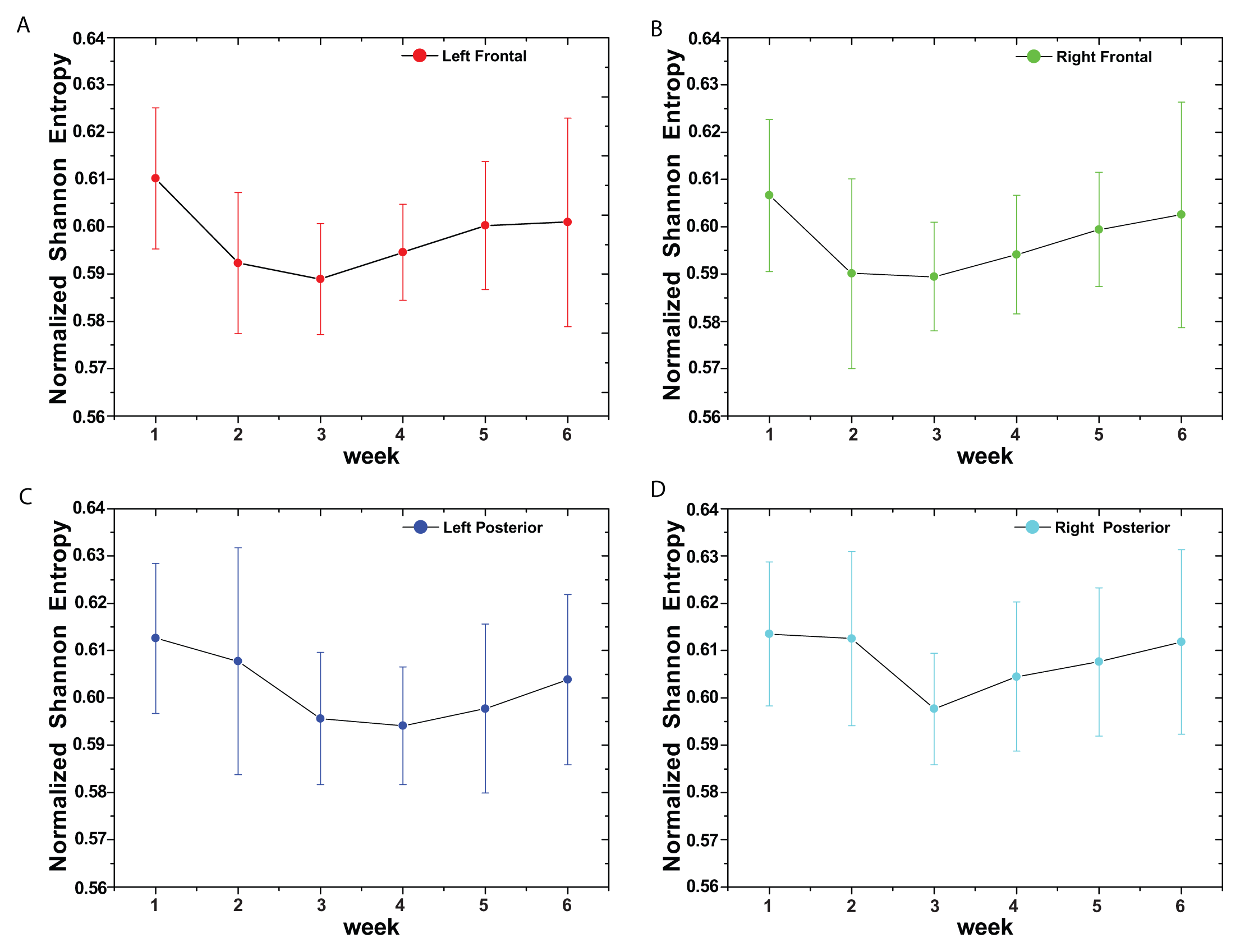
, and N the number of possible states of the system under study, the Shannon’s logarithmic information measure (Shannon entropy) [26] is defined by:
S [ P ] = - j = 1 N p j ln ( p j ) .
This functional is equal to zero when we are able to predict with full certainty which of the possible outcomes j, whose probabilities are given by pj, will actually take place. Our knowledge of the underlying process, described by the probability distribution, is maximal in this instance. In contrast, this knowledge is commonly minimal for a uniform distribution Pe = {pj = 1/N, ∀ j = 1, ···, N}. The Shannon entropy S is a measure of “global character” that is not too sensitive to strong changes in the pdf taking place in a small region. Such is not the case with the Fisher information measure [27,28]:
F [ f ] = f ( x ) 2 f ( x ) d x ,
which constitutes a measure of the gradient content of the distribution f (continuous pdf), thus being quite sensitive even to tiny localized perturbations.
The Fisher information measure can be variously interpreted as a measure of the ability to estimate a parameter, as the amount of information that can be extracted from a set of measurements, and also as a measure of the state of disorder of a system or phenomenon [28,29], its most important property being the so-called Cramer–Rao bound. It is important to remark that the gradient operator significantly influences the contribution of minute local f-variations to the Fisher information value, so that the quantifier is called a “local” one. Note that Shannon entropy decreases with a skewed distribution, while Fisher information increases in such a case. Local sensitivity is useful in scenarios whose description necessitates an appeal to a notion of “order” [1719]. The concomitant problem of loss of information due to the discretization has been thoroughly studied (see, for instance, [3032] and the references therein), and in particular, it entails the loss of Fisher’s shift-invariance, which is of no importance for our present purposes.
For Fisher information measure computation (discrete pdf), we follow the proposal of Dehesa and coworkers [33] based on amplitude of probability f(x) = ψ(x)2, then:
F [ ψ ] = 4 { d ψ d x } 2 d x .
Its discrete version is now:
F [ P ] = 4 i = 1 N - 1 ( p i + 1 - p i ) 2 .
If our system is in a very ordered state and, thus, is represented by a very narrow pdf, we have a Shannon entropy S ~ 0 and a Fisher information measure F ~ Fmax. On the other hand, when the system under study lies in a very disordered state, one gets an almost flat pdf and S ~ Smax, while F ~ 0. Of course, Smax and Fmax are, respectively, the maximum values for the Shannon entropy and Fisher information measure. One can state that the general behavior of the Fisher information measure is opposite to that of the Shannon entropy [34].
It is well known, however, that the ordinal structures present in a process is not quantified by randomness measures, and consequently, measures of statistical or structural complexity are necessary for a better understanding (characterization) of the system dynamics represented by their time series [35]. The opposite extremes of perfect order (i.e., a periodic sequence) and maximal randomness (i.e., a fair coin toss) are very simple to describe, because they do not have any structure. The complexity should be zero in these cases. At a given distance from these extremes, a wide range of possible ordinal structures exists. The statistical complexity measure allows one to quantify this array of behavior [36]. We consider the MPR complexity [37], as it is able to quantify critical details of dynamical processes underlying the data set.
Based on the seminal notion advanced by López-Ruiz et al. [38], this statistical complexity measure is defined through the functional product form:
C J S [ P ] = Q J [ P , P e ] · H S [ P ]
of the normalized Shannon entropy:
H S [ P ] = S [ P ] / S m a x
with Smax = S[Pe] = lnN, (0 ≤ HS ≤ 1) and the disequilibrium Entropy 16 04677f7J defined in terms of the Jensen–Shannon divergence. That is,
Q J [ P , P e ] = Q 0 J [ P , P e ]
with:
J [ P , P e ] = S [ ( P + P e ) / 2 ] - S [ P ] / 2 - S [ P e ] / 2
the above-mentioned Jensen–Shannon divergence and Q0, a normalization constant (0 ≤ Entropy 16 04677f7J ≤ 1), are equal to the inverse of the maximum possible value of Entropy 16 04677f8
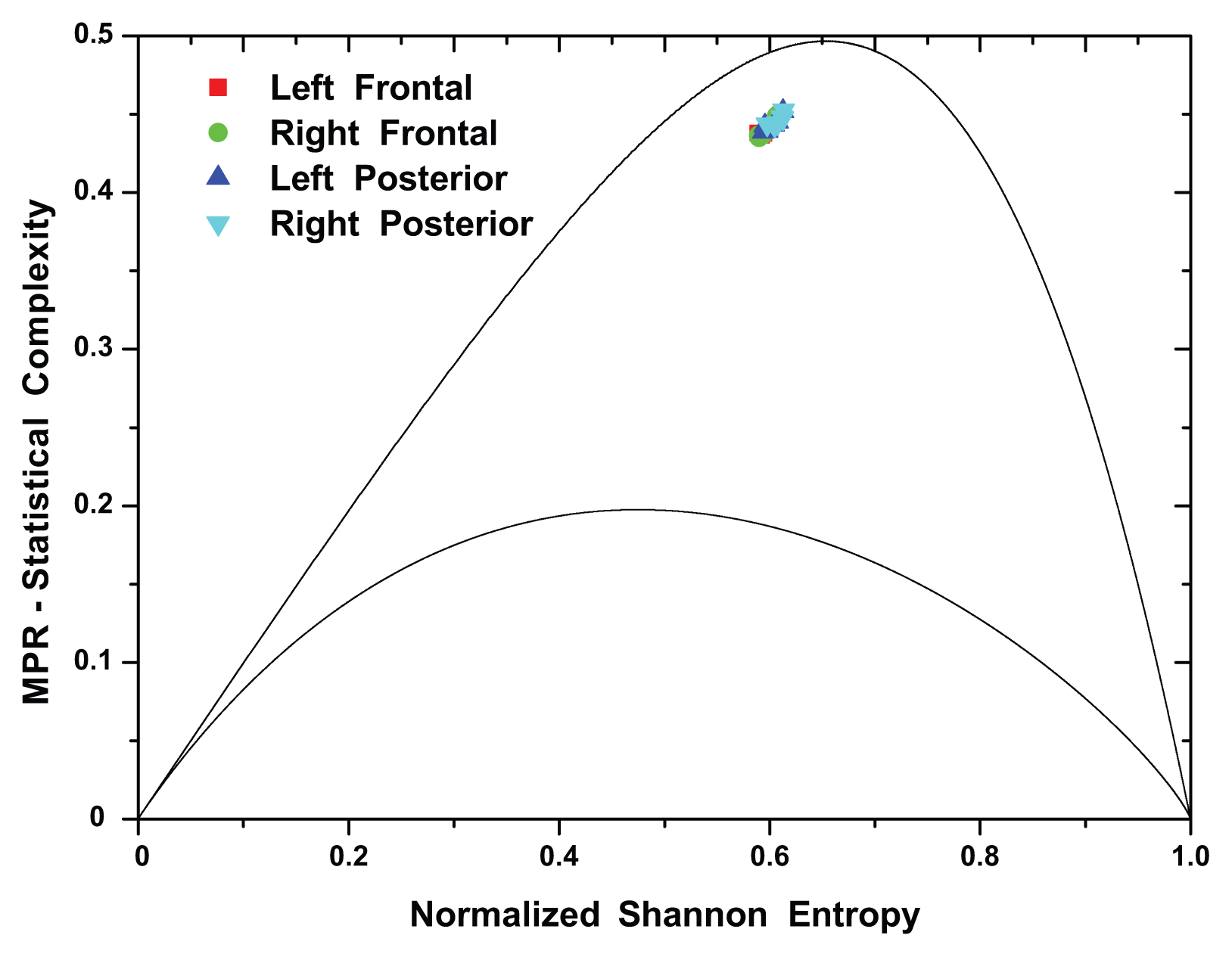
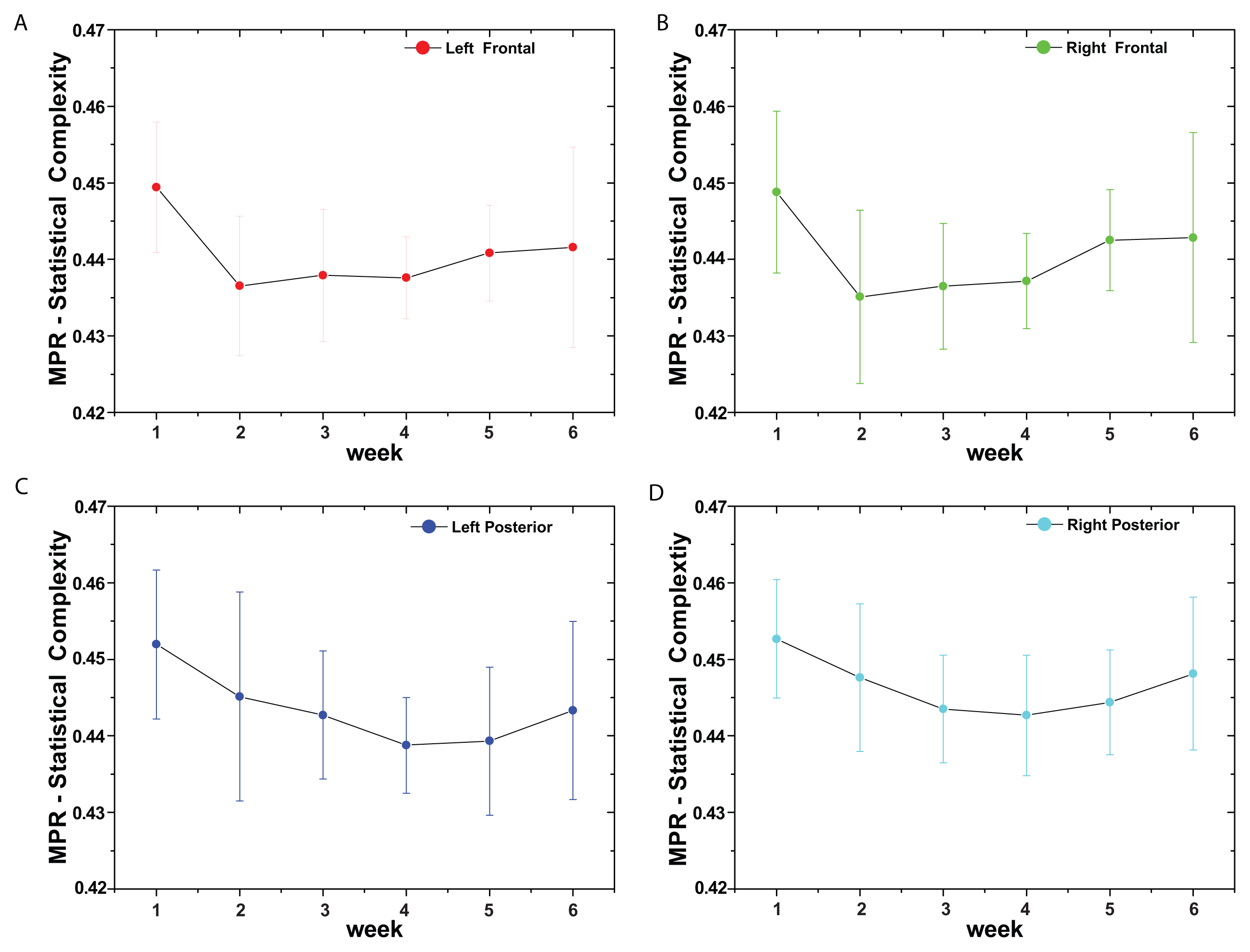
[P, Pe]. This value is obtained when one of the components of the pdf, P, say pm, is equal to one and the remaining pj are equal to zero. The Jensen–Shannon divergence, which quantifies the difference between two (or more) probability distributions, is especially useful to compare the symbolic composition between different sequences [39]. Note that the above introduced statistical complexity depends on two different probability distributions, the one associated with the system under analysis, P, and the uniform distribution, Pe. Furthermore, it was shown that for a given value of HS, the range of possible CJS values varies between a minimum Cmin and a maximum Cmax, restricting the possible values of the statistical complexity in a given entropy-complexity plane [40]. Thus, it is clear that important additional information related to the correlational structure between the components of the physical system is provided by evaluating the statistical complexity measure.

2.3. The Bandt–Pompe Approach to the pdf Determination

The study and characterization of time series Entropy 16 04677f6
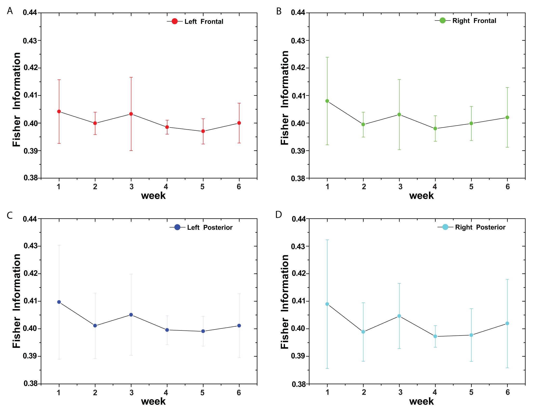
(t) by recourse to information theory tools assume that the underlying pdf is given a priori. In contrast, part of the concomitant analysis involves extracting the pdf from the data, and there is no univocal procedure with which everyone agrees. Almost ten years ago, Bandt and Pompe (BP) introduced a successful methodology for the evaluation of the pdf associated with scalar time series data using a symbolization technique [1]. For a didactic description of the approach, as well as its main biomedical and econophysics applications, see [2].
The pertinent symbolic data are: (i) created by ranking the values of the series; and (ii) defined by reordering the embedded data in ascending order, which is tantamount to a phase space reconstruction with embedding dimension (pattern length) D and time lag τ. In this way, it is possible to quantify the diversity of the ordering symbols (patterns) derived from a scalar time series.
Note that the appropriate symbol sequence arises naturally from the time series, and no model-based assumptions are needed. In fact, the necessary “partitions” are devised by comparing the order of neighboring relative values rather than by apportioning amplitudes according to different levels. This technique, as opposed to most of those in current practice, takes into account the temporal structure of the time series generated by the physical process under study. This feature allows us to uncover important details concerning the ordinal structure of the time series [19,41,42] and can also yield information about temporal correlation [15,16].
It is clear that this type of analysis of a time series entails losing some details of the original series’ amplitude information. Nevertheless, by just referring to the series’ intrinsic structure, a meaningful difficulty reduction has indeed been achieved by Bandt and Pompe with regard to the description of complex systems. The symbolic representation of time series by recourse to a comparison of consecutive (τ = 1) or nonconsecutive (τ > 1) values allows for an accurate empirical reconstruction of the underlying phase-space, even in the presence of weak (observational and dynamic) noise [1]. Furthermore, the ordinal patterns associated with the pdf is invariant with respect to nonlinear monotonous transformations. Accordingly, nonlinear drifts or scaling artificially introduced by a measurement device will not modify the estimation of quantifiers, a nice property if one deals with experimental data (see, e.g., [43]). These advantages make the Bandt and Pompe methodology more convenient than conventional methods based on range partitioning (i.e., pdf based on histograms).
Additional advantages of the method reside in: (i) its simplicity; we need few parameters: the pattern length/embedding dimension D and the embedding delay τ ; and (ii) the extremely fast nature of the pertinent calculation process [44]. The BP methodology can be applied not only to time series representative of low dimensional dynamical systems, but also to any type of time series (regular, chaotic, noisy or reality based). In fact, the existence of an attractor in the D-dimensional phase space is not assumed. The only condition for the applicability of the Bandt–Pompe methodology is a very weak stationary assumption (that is, for kD, the probability for xt < xt+k should not depend on t [1]).
To use the Bandt and Pompe [1] methodology for evaluating the pdf, P, associated with the time series (dynamical system) under study, one starts by considering partitions of the pertinent D-dimensional space that will hopefully “reveal” relevant details of the ordinal structure of a given one-dimensional time series Entropy 16 04677f6(t) = {xt; t = 1, ···, M} with embedding dimension D > 1 (D ∈ ℕ) and embedding time delay τ (τ ∈ ℕ). We are interested in “ordinal patterns” of order (length) D generated by (s) ↦ (xs− (D−1)τ, xs− (D−2)τ, ···, xsτ,xs ), which assigns to each time s the D-dimensional vector of values at times s, sτ, ···, s − (D − 1)τ. Clearly, the greater the D–value, the more information on the past is incorporated into our vectors. By “ordinal pattern” related to the time (s), we mean the permutation π = (r0, r1, ···, rD−1) of [0, 1, ···,D − 1] defined by xsrD−1τxsrD−2τ ≤ ··· ≤ xsr1τxsr0τ. In order to get a unique result, we set ri < ri−1 if xsri = xsri−1. This is justified if the values of xt have a continuous distribution, so that equal values are very unusual. Thus, for all the D! possible permutations π of order D, their associated relative frequencies can be naturally computed by the number of times this particular order sequence is found in the time series divided by the total number of sequences.
Consequently, it is possible to quantify the diversity of the ordering symbols (patterns of length D) derived from a scalar time series, by evaluating the so-called permutation entropy, the permutation statistical complexity and Fisher permutation information measure. Of course, the embedding dimension D plays an important role in the evaluation of the appropriate probability distribution, because D determines the number of accessible states D! and also conditions the minimum acceptable length MD! of the time series that one needs in order to work with reliable statistics [41].
Regarding the selection of the parameters, Bandt and Pompe suggested working with 4 ≤ D ≤ 6 and specifically considered an embedding delay τ = 1 in their cornerstone paper [1]. Nevertheless, it is clear that other values of τ could provide additional information. It has been recently shown that this parameter is strongly related, if it is relevant, to the intrinsic time scales of the system under analysis [4547].
The Bandt and Pompe proposal for associating probability distributions to time series (of an underlying symbolic nature) constitutes a significant advance in the study of nonlinear dynamical systems [1]. The method provides univocal prescription for ordinary, global entropic quantifiers of the Shannon-kind. However, as was shown by Rosso and coworkers [18,19], ambiguities arise in applying the Bandt and Pompe technique with reference to the permutation of ordinal patterns. This happens if one wishes to employ the BP-probability density to construct local entropic quantifiers, like the Fisher information measure, which would characterize time series generated by nonlinear dynamical systems.
The local sensitivity of the Fisher information measure for discrete pdfs is reflected in the fact that the specific “i-ordering” of the discrete values pi must be seriously taken into account in evaluating the sum in Equation (4). The pertinent numerator can be regarded as a kind of “distance” between two contiguous probabilities. Thus, a different ordering of the pertinent summands would lead to a different Fisher information value. In fact, if we have a discrete pdf given by P = {pi, i = 1, ···,N}, we will have N! possibilities for the i-ordering.
The question is, which is the arrangement that one could regard as the “proper” ordering? The answer is straightforward in some cases, the histogram-based pdf constituting a conspicuous example. For such a procedure, one first divides the interval [a, b] (with a and b the minimum and maximum amplitude values in the time series) into a finite number on non-overlapping sub-intervals (bins). Thus, the division procedure of the interval [a, b] provides the natural order sequence for the evaluation of the pdf gradient involved in the Fisher information measure. In our current paper, we chosen for the Bandt–Pompe pdf the lexicographic ordering given by the algorithm of Lehmer [48], amongst other possibilities, due to it provide a better distinction of different dynamics in the Fisher vs. Shannon plane (see [18,19]).

3. Results and Discussion

The application of nonlinear time series analysis provides additional information to the linear techniques as reflecting important additional information related to the correlational structure of the signal. In particular, the Bandt and Pompe technique [1] allows us to account for the ordinal structures of the EEGs time series instead of the values themselves. As we mentioned in the experimental methodology section, twenty four chickens reared from hatching were the subjects in this experiment. Four electrodes were placed over the left and right frontal (LF and RF) and left and right posterior (LP and RP) areas of the scalp with an additional reference electrode placed at the back of the head. EEG recording was taken at Day 7 posthatch and then each week for six weeks. The EEG time series studied in the current work required pre-processing in order to eliminate undesired frequencies produced by the repetitive motion (saccadic movements) typical of the studied birds. This preprocessing is not straightforward (it cannot be done with band pass filters) and was the object of a previous paper [24]. Based on the EEG signals preprocessed using a methodology of orthogonal wavelets, we estimated subtle measures accounting for their causal information: the normalized Shannon permutation entropy, Fisher permutation information and permutation statistical complexity. This allows us to investigate how the information of the system behaves as chickens reach their neurological maturity.
More specifically, in this section, we use the Bandt and Pompe [1] methodology for evaluating the pdf, P, associated with the time series, considering an embedded dimension/pattern length D = 6 (with τ = 1) and using the lexicographic pattern-ordering proposed by Lehmer [48]. This embedded dimension is enough to efficiently capture causality information of the ordinal structure of the time series [1].
In order to illustrate our methodology, Figure 1A–D shows averaged values (over all of the chickens) of the normalized Shannon permutation entropy and its standard deviation versus the maturation week when considering the recordings of the four electrodes. Note that the normalized permutation Shannon entropy mean value decreases up to the third week, but thereafter grows closer to its initial value. Figure 2A–D shows that mean values permutation Fisher information (and its standard deviation) does not show significative changes as the chicken brain reaches its maturity. Figure 3A–D shows that permutation MPR statistical complexity mean values decreases up to the third week, but thereafter grows closer to its initial value.
Figure 4A–D shows the informational causal plane of entropy versus complexity, H × C. Note that the MPR permutation statistical complexity and normalized permutation Shannon entropy decrease up to the third week. That is, during the three first weeks, the system, instead of developing into a more complex state, moves to lower values, producing its entropic reduction, where it reaches a more ordered state. After that, the normalized permutation Shannon entropy grows to higher values where the system reaches a greater entropic deterioration together with a higher level of permutation statistical complexity.
MPR permutation complexity is a measure derived from nonlinear systems theory that, when applied to EEG signals, can be indicative of the global dynamical complexity of electrocortical activity. However, to obtain further understanding of our results, we need to plot the localization in the causality entropy-complexity plane of the results obtained in the present work. Figure 5 displays all of the results considered here in the causality entropy-complexity plane H×C location. The continuous lines represent the curves of maximum and minimum statistical complexity, Cmax and Cmin, respectively, as functions of the normalized Shannon entropy [40]. A closer look reveals that our results are in the chaotic attractors zone, corresponding to the localization of a dissipative chaotic system. As can be appreciated from the contrast of our results with the one being shown in [42], in which the Bandt–Pompe pdf was evaluated considering D = 6 (pattern length), τ = 1 (time lag), our results correspond to the localization of a chaotic dissipative system: the Tinkerbell map X-component [42].
EEGs reflect the electrical activity of the brain, and the problem of analyzing and interpreting the meaning of these signals has received a great deal of attention. Since EEG signals may be considered chaotic, nonlinear theory can provide effective quantitative descriptors of EEG dynamics and of underlying chaos in the brain. However, choosing the appropriate methodology to characterize the chaotic behavior can be a difficult task. Biochemical, morphological and physiological data indicate that the forebrain of chickens exhibits a protracted period of maturation [2022], and this temporal separation of the synapse formation and maturation phases is analogous to human neural development, though the changes in chickens occur in weeks compared with years in humans.
In this paper, we have shown that the complexity of the electrical activity of the chicken brain can be characterized by estimating the intrinsic correlational structure of the EEG signal through the MPR statistical complexity [15,16]. In particular, the causal entropy-complexity plane H × C allows us to identify the localization of the developing chicken brain dynamics within the zone of a chaotic dissipative behavior. We have shown that MPR permutation statistical complexity and normalized Shannon permutation entropy decrease up to the third week. More specifically, during the three first weeks, the system moves to lower complexity together with an entropic reduction where the network reduces the level of chaos as synapse formation is established. Afterward, the system reaches a greater entropic deterioration together with a higher level of complexity, suggesting that chicken brains display a critical level of complexity consistent with their emergent functions. This behavior is associated with the “maturation period” described by Rostas a co-workers [21,22]. Thus, Shannon entropy and the MPR statistical complexity measure not only provide a robust method to analyze EEG signals, but also advance the classification of mental states, distinguishing normal behavioral pattern from anomalies that may cause dysfunction.

4. Conclusions

Animal models provide an invaluable source of information in the testing of hypotheses that are difficult to corroborate by other experimental means. In the present work, we revisit the data analysis of scalp-applied recording electrodes that have been used to monitor changes in basal EEG patterns in chickens during posthatch development [23]. Unfortunately, the literature on the use of the EEG in the chicken is not extensive. Research efforts have largely concerned the use of the EEG either as an indicator of the general integrity of the nervous system or as a measure of specific brain states, such as sleep cycles and other EEG rhythm-defined states. In those studies using the EEG as a functional integrity measure of the chicken nervous system, a major interest has been to plot the embryonic development of the chicken brain. The functional properties of synaptic networks and the signaling machinery in neurons are known to change during development, and it is thought that these changes are important for the plasticity that brings about the fine-tuning of neuronal circuits during the maturation of the brain.
In recent years, there has been a growing realization that the development of synaptic networks in the brain can be regarded as occurring in two broadly defined phases. During the initial synapse formation phase, functional synaptic contacts are established in a changing tissue environment, and there is a net increase in the number of synapses. In the subsequent maturation phase, during which the tissue environment is broadly stable, except for an increase in myelination, there is little change in synapse number in the brain overall, but immature, yet functional, synapses are altered to become like those found in the adult, brain with synaptic circuits being fine-tuned [21,22]. Synapse formation in the chicken brain occurs most rapidly around the time of hatching, and it is complete by 10 to 14 days posthatch [49]. Subsequently, the immature synapses and neurons gradually attain adult ultrastructural and biochemical properties. These changes occur in the period between three and eight weeks posthatch, during which neuronal circuits become fine-tuned, and have been termed the “maturation period” by Rostas [21]. That is, during the second period, neuronal circuits become fine-tuned.
According to the theorem of Liouville in the case of dissipative systems (non-energy preserving), the volume occupied by the states in the phase space shrinks as time goes towards infinity. The limit set of an autonomous dissipative system to which trajectories converge for time increasing towards infinity is called the attractor. As the chicken brain develops, dendrites dissipate large quantities of their metabolic energy. Dissipation in this case manifests itself in the disappearance of energy and the emergence of a complex network structure. In this paper, we show that the development of the chicken brain could be thought of as a dissipative chaotic system in which the network dynamics during development is associated with a complex structure reflected in the causality entropy-complexity plane, H × C.
We have investigated the development and maturation of brain functions using information theory-based tools [15,16], showing that the complexity of the electrical activity can be characterized by estimating the intrinsic correlational structure of the EEG signal. Our current approach allows us to distinguish two broadly-defined phases. More specifically, during the first phase, which corresponds to the three first weeks, the system moves to lower complexity together with an entropic reduction (where the network reaches a more ordered state). Thereafter, in the second phase, the system reaches a greater entropic deterioration together with a higher level of complexity. In the second phase, the relevant structures of the brain reach a critical level of maturation together with a higher level of complexity, in conformity to the behavioral changes occurring throughout this period [21,22].
A mental disorder, also called a mental illness or a psychiatric disorder, is a mental or behavioral pattern or anomaly. Future research should examine how developmental changes, such as an induced illness or due to inappropriate nutrition, or detrimental effects on cognitive functions can modify the complexity measures during the development of the chicken brain. Thus, using normalized Shannon entropy and MPR complexity, EEG signals can be important tools, not only for interpreting brain coding dynamics, but also for diagnosing mental diseases.

Acknowledgments

The authors gratefully acknowledge John A.P. Rostas and Mick Hunter, The University of Newcastle, Australia, for allowing us to use their EEG chicken data. Osvaldo A. Rosso and Fernando Montani are members of the National Research Career of CONICET Argentina. Research supported by PIP (Proyecto de Investigación Plurianual) 0255/11 CONICET, Argentina (Fernando Montani). Osvaldo A. Rosso acknowledges the support of FAPEAL (Fundaçâo de Amparo ã Pesquisa do Est de Alagoas), Brazil.

Author Contributions

Fernando Montani and Osvaldo A. Rosso contributed equally in the design of this research as well as in the writing of this paper. Both authors have read and approved the final manuscript.

Conflicts of Interest

The authors declare no conflict of interest.

References

  1. Bandt, C.; Pompe, B. Permutation entropy: A natural complexity measure for time series. Phys. Rev. Lett 2002, 88, 174102. [Google Scholar]
  2. Zanin, M.; Zunino, L.; Rosso, O.A.; Papo, D. Permutation Entropy and Its Main Biomedical and Econophysics Applications: A Review. Entropy 2012, 14, 1553–1577. [Google Scholar]
  3. Schindler, K.; Gast, H.; Stieglitz, L.; Stibal, A.; Hauf, M.; Wiest, R.; Mariani, L.; Rummel, C. Forbidden ordinal patterns of periictal intracranial EEG indicate deterministic dynamics in human epileptic seizures. Epilepsia 2011, 52, 1771–1780. [Google Scholar]
  4. Veisi, I.; Pariz, N.; Karimpour, A. Fast and Robust Detection of Epilepsy in Noisy EEG Signals Using Permutation Entropy. Proceedings of the 7th IEEE International Conference on Bioinformatics and Bioengineering, Boston, MA, USA, 14–17 October 2007; pp. 200–203.
  5. Cao, Y.; Tung, W.; Gao, J.B.; Protopopescu, V.A.; Hively, L.M. Detecting dynamical changes in time series using the permutation entropy. Phys. Rev. E 2004, 70, 046217. [Google Scholar]
  6. Ouyang, G.; Dang, C.; Richards, D.A.; Li, X. Ordinal pattern based similarity analysis for EEG recordings. Clin. Neurophysiol 2010, 121, 694–703. [Google Scholar]
  7. Bruzzo, A.A.; Gesierich, B.; Santi, M.; Tassinari, C.; Birbaumer, N.; Rubboli, G. Permutation entropy to detect vigilance changes and preictal states from scalp EEG in epileptic patients: A preliminary study. Neurol. Sci 2008, 29, 3–9. [Google Scholar]
  8. Li, X.; Cui, S.M.E.; Voss, L.J. Using permutation entropy to measure the electroencephalographic effect of sevoflurane. Anesthesiology 2007, 109, 448–456. [Google Scholar]
  9. Olofsen, E.; Sleigh, J.W.; Dahan, V. Permutation entropy of the electroencephalogram: A measure of anaesthetic drug effect. Br. J. Anaesth 2008, 101, 810–821. [Google Scholar]
  10. Jordan, D.; Stockmanns, G.; Kochs, E.F.; Pilge, S.; Schneider, G. Electroencephalographic order pattern analysis for the separation of consciousness and unconsciousness: An analysis of approximate entropy, permutation entropy, recurrence rate, and phase coupling of order recurrence plots. Anesthesiology 2008, 109, 1014–1022. [Google Scholar]
  11. Nicolaou, N.; Georgiou, J. Detection of epileptic electroencephalogram based on Permutation, Entropy and Support Vector Machines. Expert Syst. Appl 2012, 39, 202–209. [Google Scholar]
  12. Robinson, S.E.; Mandell, A.J.; Coppola, R. Spatiotemporal imaging of complexity. Front. Comput. Neurosci 2013, 101, 1–14. [Google Scholar]
  13. Schröter, M.S.; Spoormaker, V.I.; Schorer, A.; Wohlschläger, A.; Czisch, M.; Kochs, E.F.; Zimmer, C.; Hemmer, B.; Schneider, G.; Jordan, D.; Ilg, R. Spatiotemporal Reconfiguration of Large-Scale Brain Functional Networks during Propofol-Induced Loss of Consciousness. J. Neurosci 2012, 32, 12832–12840. [Google Scholar]
  14. Rummel, C.; Abela, E.; Hauf, M.; Wiest, R.; Schindler, K. Ordinal patterns in epileptic brains: Analysis of intracranial EEG and simultaneous EEG-fMRI. Eur. Phys. J. Spec. Top 2013, 222, 569–585. [Google Scholar]
  15. Rosso, O.A.; Masoller, C. Detecting and quantifying stochastic and coherence resonances via information-theory complexity measurements. Phys. Rev. E 2009, 79, 040106(R). [Google Scholar]
  16. Rosso, O.A.; Masoller, C. Detecting and quantifying temporal correlations in stochastic resonance via information theory measures. Eur. Phys. J. B 2009, 69, 37–43. [Google Scholar]
  17. Rosso, O.A.; De Micco, K.; Plastino, A.; Larrondo, H. Info-quantifiers’ map-characterization revisited. Physica A 2010, 389, 249–262. [Google Scholar]
  18. Olivares, F.; Plastino, A.; Rosso, O.A. Ambiguities in the Bandt-Pompe’s methodology for local entropic quantifiers. Physica A 2012, 391, 2518–2526. [Google Scholar]
  19. Olivares, F.; Plastino, A.; Rosso, O.A. Contrasting chaos with noise via local versus global information quantifiers. Phys. Lett. A 2012, 376, 1577–1583. [Google Scholar]
  20. Changeux, J.P.; Courrege, P.; Danchin, A. A theory of the epigenesis of neuronal networks by selective stabilization of synapses. Proc. Natl. Acad. Sci. USA 1973, 70, 2974–2978. [Google Scholar]
  21. Rostas, J.A.P.; Kavanagh, J.M.; Dodd, P.R.; Heath, J.W.; Powis, D.A. Mechanisms of synaptic plasticity. Changes in postsynaptic densities and glutamate receptors in chicken forebrain during maturation. Mol. Neurobiol 1991, 5, 203–216. [Google Scholar]
  22. Rostas, J.A.P. Molecular mechanisms of neuronal maturation: A model for synaptic plasticity. In Neural and Behavioural Plasticity: The Use of the Domestic Chick as a Model; Andrew, R.J., Ed.; Oxford University Press: Oxford, UK, 1991; pp. 177–201. [Google Scholar]
  23. Hunter, M.; Battilana, M.; Bragg, T.; Rostas, J.A.P. EEG as a measure of developmental changes in the chicken brain. Dev. Psychobiol 2000, 36, 23–28. [Google Scholar]
  24. Figliola, A.; Rosso, O.A.; Serrano, E. Atenuacion de frecuencias indeseadas usando transformada wavelet. Proceedings of XI Reunión de Trabajo en Procesamiento de la Información y Control; Grupo de Electronica Aplicada: Rio Cuarto, Córdoba, Argentina, 2005; pp. 28–32. (In Spanish)[Google Scholar]
  25. Fernandez, J.G.; Larrondo, H.A.; Figliola, A.; Serrano, E.; Rostas, J.A.P.; Hunter, M.; Rosso, O.A. Brain maturation changes characterized by algorithmic complexity (Lempel and Zip complexity). In AIP Conference Proceedings; Descalzi, O., Larrondo, H.A., Rosso, O.A., Eds.; American Institute of Physics: New York, NY, USA, 2007; pp. 196–202. [Google Scholar]
  26. Shannon, C.; Weaver, W. The Mathematical Theory of Communication; University of Illinois Press: Champaign, IL, USA, 1949. [Google Scholar]
  27. Fisher, R.A. On the mathematical foundations of theoretical statistics. Philos. Trans. R. Soc. Lond. Ser. A 1922, 222, 309–368. [Google Scholar]
  28. Frieden, B.R. Science from Fisher information: A Unification; Cambridge University Press: Cambridge, UK, 2004. [Google Scholar]
  29. Mayer, A.L.; Pawlowski, C.W.; Cabezas, H. Fisher Information and dinamic regime changes in ecological systems. Ecol. Model 2006, 195, 72–82. [Google Scholar]
  30. Zografos, K.; Ferentinos, K.; Papaioannou, T. Discrete approximations to the Csiszár, Renyi, and Fisher measures of information. Can. J. Stat 1986, 14, 355–366. [Google Scholar]
  31. Pardo, L.; Morales, D.; Ferentinos, K.; Zografos, K. Discretization problems on generalized entropies and R-divergences. Kybernetika 1994, 30, 445–460. [Google Scholar]
  32. Madiman, M.; Johnson, O.; Kontoyiannis, I. Fisher Information, compound Poisson approximation, and the Poisson channel. Proceedings of the IEEE International Symposium on Information Theory, 2007 (ISIT 2007), Nice, France, 24–29 June 2007; pp. 976–980.
  33. Sanchez-Moreno, P.; Dehesa, J.S.; Yanez, R.J. Discrete Densities and Fisher Information. In Difference Equations and Applications, Proceedings of the 14th International Conference on Difference Equations and Applications; Uğur-Bahçeşehir University Publishing Company: Istanbul, Turkey, 2009; pp. 291–298. [Google Scholar]
  34. Pennini, F.; Plastino, A. Reciprocity relations between ordinary temperature and the Frieden-Soffer Fisher temperature. Phys. Rev. E 2005, 71, 047102. [Google Scholar]
  35. Feldman, D.P.; Crutchfield, J.P. Measures of Statistical Complexity: Why? Phys. Lett. A 1998, 238, 244–252. [Google Scholar]
  36. Feldman, D.P.; McTague, C.S.; Crutchfield, J.P. The organization of intrinsic computation: Complexity-entropy diagrams and the diversity of natural information processing. Chaos 2008, 18, 043106. [Google Scholar]
  37. Lamberti, P.W.; Martín, M.T.; Plastino, A.; Rosso, O.A. Intensive entropic non-triviality measure. Physica A 2004, 334, 119–131. [Google Scholar]
  38. López-Ruiz, R.; Mancini, H.L.; Calbet, X. A statistical measure of complexity. Phys. Lett. A 1995, 209, 321–326. [Google Scholar]
  39. Grosse, I.; Bernaola-Galván, P.; Carpena, P.; Román-Roldán, R.; Oliver, J.; Stanley, H.E. Analysis of symbolic sequences using the Jensen-Shannon divergence. Phys. Rev. E 2002, 65, 041905. [Google Scholar]
  40. Martín, M.T.; Plastino, A.; Rosso, O.A. Generalized statistical complexity measures: Geometrical and analytical properties. Physica A 2006, 369, 439–462. [Google Scholar]
  41. Rosso, O.A.; Larrondo, H.A.; Martín, M.T.; Plastino, A.; Fuentes, M.A. Distinguishing noise from chaos. Phys. Rev. Lett 2007, 99, 154102. [Google Scholar]
  42. Rosso, O.A.; Olivares, F.; Zunino, L.; De Micco, L.; Aquino, A.L.L.; Plastino, A.; Larrondo, H.A. Characterization of chaotic maps using the permutation Bandt-Pompe probability distribution. Eur. Phys. J. B 2012, 86, 116–129. [Google Scholar]
  43. Saco, P.M.; Carpi, L.C.; Figliola, A.; Serrano, E.; Rosso, O.A. Entropy analysis of the dynamics of El Niño/Southern Oscillation during the Holocene. Physica A 2010, 389, 5022–5027. [Google Scholar]
  44. Keller, K.; Sinn, M. Ordinal Analysis of Time Series. Physica A 2005, 356, 114–120. [Google Scholar]
  45. Zunino, L.; Soriano, M.C.; Fischer, I.; Rosso, O.A.; Mirasso, C.R. Permutation-information -theory approach to unveil delay dynamics from time-series analysis. Phys. Rev. E 2010, 82, 046212. [Google Scholar]
  46. Soriano, M.C.; Zunino, L.; Rosso, O.A.; Fischer, I.; Mirasso, C.R. Time Scales of a Chaotic Semiconductor Laser with Optical Feedback Under the Lens of a Permutation Information Analysis. IEEE J. Quantum Electron 2001, 47, 252–261. [Google Scholar]
  47. Zunino, L.; Soriano, M.C.; Rosso, O.A. Distinguishing chaotic and stochastic dynamics from time series by using a multiscale symbolic approach. Phys. Rev. E 2012, 86, 046210. [Google Scholar]
  48. FactoradicPermutation.hh. Available online: http://www.keithschwarz.com/interesting/code/factoradic-permutation/FactoradicPermutation (accessed 21st September 2011).
  49. Rostas, J.A.P.; Kavanagh, J.M.; Dodd, P.R.; Heath, J.W.; Powis, D.A. Mechanisms of synaptic plasticity. Mol. Neurobiol 1992, 5, 203–216. [Google Scholar]
Figure 1. Normalized permutation Shannon Entropy versus the maturation week (average values and standard deviation estimated considering the 24 chickens). The used pdf Bandt–Pompe parameters are D = 6 and τ = 1. (A) Left frontal electrode. (B) Right frontal electrode. (C) Left posterior electrode. (D) Right posterior electrode.
Entropy 16 04677f1
Figure 2. Permutation Fisher information versus the maturation week (average values and standard deviation estimated considering the 24 chickens). The used pdf Bandt–Pompe parameters are D = 6 and τ = 1. (A) Left frontal electrode. (B) Right frontal electrode. (C) Left posterior electrode. (D) Right posterior electrode.
Entropy 16 04677f2
Figure 3. MPRpermutation statistical complexity versus the maturation week (average values and standard deviation estimated considering the 24 chickens). The used pdf Bandt–Pompe parameters are D = 6 and τ = 1. (A) Left frontal electrode. (B) Right frontal electrode. (C) Left posterior electrode. (D) Right posterior electrode.
Entropy 16 04677f3
Figure 4. Causality entropy-complexity plane H × C: localization of the mean values. We used an embedding dimension of D = 6 and a time lag of τ = 1 to estimate the pdf associated with the Bandt–Pompe methodology. (A) Left frontal electrode. (B) Right frontal electrode. (C) Left posterior electrode. (D) Right posterior electrode.
Entropy 16 04677f4
Figure 5. Localization in the causality entropy-complexity plane of the EEGs results presented in this work. Note that our results are localized in a chaotic dissipative behavior zone [42].
Entropy 16 04677f5

