1. Introduction
In this article, we present the results of an exploratory computational study of a possible instability in the Richtmyer–Meshkov flow over a surface deflection in a warm dense plasma environment. Over the past several decades, powerful laser facilities have been constructed to provide the hot dense matter required for the initiation of inertial fusion (Atzeni, Meyer-ter-Vehn [
1], Drake [
2]). Additional laser facilities have been implemented to support this effort and are capable of providing the warm dense matter required to simulate the environment found in supernova plasma [
2]. Results obtained from these facilities have confirmed the existence of the Rayleigh–Taylor instability (buoyancy effect between two adjacent layers), the Kelvin–Helmholtz instability (the effect of shear between adjacent layers), and the Richtmyer–Meshkov instability (induced parallel flow due to surface ripples) [
2]. Recently, Harding [
3] presented the results of a carefully conducted experimental study of the Richtmyer–Meshkov effect using the absorption of laser energy in an Al foil over a foam substrate. These results demonstrate that a rippled foam surface represents a flow deflection, resulting in a strong oblique shock wave and an induced parallel flow over the deflected foam surface (Richtmyer–Meshkov effect) [
3]. These results also indicate the possible presence of an instability not accounted for by the three processes listed above. The three cited references provide an extensive bibliography to the literature in this field of study.
In the study reported here, the warm dense plasma environment is modeled as a supersonic flow through a strong oblique shock wave produced by a wedge deflection of the flow [
3]. The three-dimensional laminar boundary layer along the wedge surface is computed by well-established computer procedures as presented in detail by Cebeci and Bradshaw [
4] and Cebeci and Cousteix [
5]. The fluctuating velocity equations are Fourier-transformed into Lorenz-form and time-integrated with the mean velocity gradients from the boundary layer solutions serving as input parameters. The singular value decomposition method provides the fraction of kinetic energy distributed over the empirical modes of the decomposition of the deterministic structures predicted by the integration of the Fourier spectral equations for the fluctuating velocity wave components. The introduction of the empirical entropic index, and the subsequent evaluation of the intermittency exponent provide a connecting link from the predicted deterministic structures to the computation of the entropy generation rate through the dissipation of the kinetic energy to thermal energy within the deterministic structures.
This article is presented with the following sections:
In Section 2, we discuss the warm dense plasma conditions produced by a strong oblique shock process (Atzeni and Meyer-ter-Vehn [
1], Drake [
2], Harding [
3], Zucrow and Hoffman [
6]) and the computational results for the thermo-transport properties (Sonntag and Van Wylen [
7], Chase [
8], Spitzer [
9], Cambel [
10]) that are used throughout the computational processes. The boundary layer flow environment that forms the basis for the evaluation of boundary layer deterministic structures is presented in Section 3. In Section 3, we assume that our flow environment is a three-dimensional laminar flow over a flat plate with a constant velocity in the streamwise (along the x-axis) direction, with no pressure gradient, and that the flow is incompressible (Isaacson [
11]). We assume a weak cross-flow velocity created by asymmetry in the surface ripple. The laminar boundary layer development is computed from the starting point of the surface ripple, providing a priori the three-dimensional boundary layer velocity profiles at various stations in the streamwise direction (Cebeci and Bradshaw [
4], Isaacson [
12], Hansen [
13]). In Section 4, the Townsend equations [
14] are written for all three fluctuating velocity components within the given three-dimensional boundary layer flow. These equations are Fourier transformed into a set of deterministic equations (Hellberg and Orszag [
15], Isaacson [
16], Manneville [
17]) from which the time-dependent behavior of the both the Fourier components of the wave number vectors and the Fourier components of the fluctuating velocity wave vectors are obtained. The results for these computations are presented in Section 5. The power spectral density of the resulting non-linear time series solution for the streamwise velocity wave component is presented in Section 6 (Chen [
18], Cover and Thomas [
19], Rissanen [
20,
21], Li and Vitanyi [
22]). The results for the singular value decomposition of selected regions of the nonlinear time series solutions are presented in Section 7 (Holmes
et al. [
23]). From these results, empirical entropy is defined for each of the empirical modes obtained in the computation [
11,
20]. In Section 8, the empirical entropic index (Tsallis [
24]) is computed from the empirical entropy value for each empirical mode ([
11,
20], Mariz [
25], Glansdorff and Prigogine [
26]). Section 9 presents the intermittency exponent (Arimitsu and Arimitsu [
27], Mathieu and Scott [
28]) from the associated empirical entropic index for each empirical mode of the singular value decomposition process (Press
et al. [
29], Isaacson [
31]). Section 10 presents the calculation of the entropy generation rate (de Groot and Mazur [
34], Truitt [
35], Bejan [
36]) through the dissipation of the appropriate part of the total kinetic energy applied as input to the original deterministic structures produced within the three-dimensional boundary layer environment (Fung and Vassilicos [
37], Hurst and Vassilicos [
38], Seoud and Vassilicos [
39], Mazellier and Vassilicos [
40] and Valente and Vassilicos [
41]). The article closes with a discussion of the results and final conclusions.
2. Warm Dense Plasma Environment
Harding [
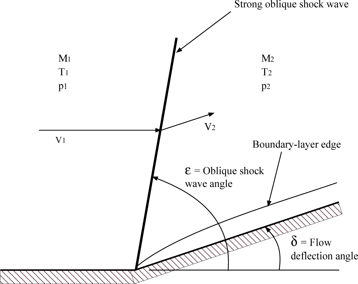
3] has suggested that the Richtmyer–Meshkov flow over a rippled surface may be represented as the flow produced by a strong oblique shock produced by a wedge-type flow deflection of an upstream supersonic flow environment. The gas dynamic analysis for this type of supersonic flow deflection, with a complete configuration of the flow environment, has been presented in [
6] (pp. 356–369). The flow environment that we consider, as shown in
Figure 1, for the computation of the entropy generation through deterministic boundary layer structures is assumed to be the supersonic flow of warm dense plasma over a two-dimensional wedge of deflection angle δ. The plasma is assumed to be a mixture of atomic hydrogen, H, ionic hydrogen, H
+, and electrons, e
−, in chemical equilibrium. The equilibrium composition and the thermodynamic properties are computed using the statistical thermodynamic methods outlined by Sonntag and Van Wylen [
7]. The statistical parameters required in these calculations are obtained from the NIST-JANAF Thermochemical Tables [
8]. The transport properties of the mixture are computed using the expressions given by Spitzer [
9].
The incoming Mach number is assumed to be 2.80, with an incoming flow temperature of 1.0 × 10
5 K and a static pressure of 4.6 × 10
9 N/m
2. For the upstream Mach number of 2.80, a wedge deflection angle of 18°, and a ratio of specific heats of 1.54, the equations of gas dynamics [
6] yield a strong oblique shock wave at a shock wave angle of approximately 81°. The subsonic, deflected flow downstream of this strong oblique shock wave is now considered as our warm dense plasma environment.
Table 1 presents the thermodynamic and transport properties used throughout the computational procedures.
3. Boundary-Layer Development
From the experimental results presented by Harding [
3], we assume that the Richtmyer–Meshkov flow downstream of the strong oblique shock wave forms a laminar boundary layer over the foam substrate surface. We also assume that additional asymmetric ripples on the substrate surface produce a weak spanwise cross-flow to the streamwise laminar boundary layer. The resulting three-dimensional boundary layer flow over the substrate surface is assumed to consist of a spatially developing Blasius boundary layer in the downstream x-y plane, and a weak spanwise Blasius boundary layer in the z-y plane. A schematic diagram of the assumed three-dimensional boundary layer configuration may be found in [
11]. Cebeci and Bradshaw [
5] present computer source codes for the numerical solutions for both laminar and turbulent boundary layers over the substrate surface. The equations required for the laminar boundary layer mean velocity gradients have been presented in [
12]. The mean boundary-layer velocity gradients serve as control parameters for the solution of the non-linear coupled Lorenz-type equations for the prediction of instabilities within the three-dimensional boundary layer environment.
The mathematical and computational procedures for the solution of the boundary layer flow equations have been presented in [
12]. However, it is our intention in this article to provide a consistent mathematical basis for the overall computational procedure used for the determination of the entropy generation by deterministic boundary layer structures. Therefore, we have included a summary of the essential equations used by Cebeci and Bradshaw [
4]. The momentum equation for the streamwise boundary-layer flow, including the contributions from both laminar and turbulent flows, may be written as:
The definitions of the terms in this equation are found in the Nomenclature. In
Equation (1), the term
represents the streamwise boundary layer stress produced by the correlation of the streamwise and the normal fluctuating velocity components. We have included this term in the development because we will use the computation of the turbulent boundary layer at the streamwise station of interest to compute the rate of entropy generation by the turbulent boundary layer at that station.
The Reynolds shear stress for the computation of turbulent boundary layers is modeled with the “eddy viscosity”,
εm, having the dimensions of (viscosity)/(density), by:
The computer program we have chosen to implement for the solution of the streamwise boundary layer equation (
Equation (1)) is based on the Keller–Cebeci box method presented by Cebeci and Bradshaw [
4] and Cebeci and Cousteix [
5]. One of the basic aspects of this method is to transform
Equation (1) into a system of first-order ordinary differential equations. The Falkner–Skan transformation, in the form:
is introduced into the transformation process. The dimensionless stream function, f(x, η), is defined by:
These definitions yield the results for the mean boundary layer velocities
u and
v as:
Differentiation with respect to η is indicated by the prime in these expressions. From Bernoulli’s equation, the pressure gradient term is given by
. To simplify the resulting equations, the parameter
m is defined as:
After a rather lengthy transformation process, (we refer the reader to Cebeci and Bradshaw [
4] for the details) the basic partial differential equation for the boundary layer (
Equation (1)) is replaced with three first-order partial nonlinear differential equations in the following form:
Cebeci and Bradshaw [
4] discuss in detail the numerical solution of the system of first-order differential equations,
Equations (9)–
(11). An arbitrary rectangular net using “centered-difference” derivatives and averages at the midpoints of net rectangles and net segments, as required, are used to get a resulting set of finite-difference equations. Newton’s method is then used to solve the resulting system of equations.
The computational procedure developed by Cebeci and Bradshaw [
4] has been used as the basis for our computations of the three-dimensional laminar boundary layer flow. The streamwise flow is of the Falkner–Skan type with an initial free stream velocity of unity, making the boundary layer edge velocity dimensionless. The main computer program in the computational procedure establishes various station numbers for the streamwise direction and assigns vertical grid numbers for the calculation of the vertical profiles at a given streamwise station. The computational domain in the streamwise direction uses stations separated by spaces of 0.02 dimensionless units beginning at the initial edge of the boundary layer development. The spanwise flow has a freestream velocity approximately ten percent of the streamwise velocity. The computational domain in the spanwise direction uses stations in increments of 0.00075 dimensionless units in the spanwise direction.
Hansen [
13] has shown that the laminar boundary layers along the starting planes for the x-y and z-y planes are similar in nature. This similarity allows the computation of the laminar mean velocity profiles in both the x-y and the z-y planes. The laminar velocity profiles in the z-y plane are computed at the fourth spanwise station, z = 0.003, and in the x-y plane at the fourth streamwise station, x = 0.08.
The gradients for the boundary layer mean velocity components are obtained from the computational results for both the streamwise boundary layer and the spanwise boundary layer. These gradients then serve as control parameters for the solution of the nonlinear time-dependent Townsend equations for the fluctuating velocity wave components in the boundary layer environment. The three-dimensional field of mean boundary layer velocity gradients serves as a computational container in which the fluctuating velocity field is placed. Thus, the three-dimensional field of boundary-layer mean velocity gradients provides the control parameters required for the solution of the Lorenz-type time-dependent coupled fluctuating velocity wave component equations. These non-linear time-series solutions indicate the presence of deterministic structures within the boundary layer flow.
4. Equations of Lorenz Form for the Spectral Velocity Wave Components
The primary hypothesis of this article is that a three-dimensional laminar boundary layer with a weak spanwise or cross-flow velocity will induce instabilities within the boundary layer leading to the development of deterministic structures within the boundary layer flow. These instabilities arise through the nonlinear interactions among the streamwise velocity fluctuations and the spanwise and normal velocity fluctuations within the laminar boundary layer flow. Separating the equations of motion into steady and unsteady equations, the equations for the velocity fluctuations may then be written as [
14–
16]:
In these equations,
ρ is the density and
v is the kinematic viscosity,
Ui represent the mean velocity components with
i = 1, 2, 3 indicating the x, y, and z components, and
xj, with
j = 1, 2, 3, designate the x, y and z directions. The pressure term is eliminated by taking the divergence of
Equation (13) and invoking incompressibility, yielding:
The equations for the velocity and pressure fluctuations represent the variables of interest in the physical plane. However, the computational procedures we employ require the equations to be in the spectral plane. The solution of the spectral equations yields the fluctuating wave vector components and the fluctuating velocity wave components. The statistical analysis of the nonlinear time series solution for the streamwise velocity wave component involves the product of these components. Through Parseval’s theorem, the spectral fluctuating velocity component products also represent the products of the streamwise fluctuating velocity components in the physical plane. These quadratic terms in the physical plane are then applied to the determination of the entropy generation rate in the thermodynamic analysis of the irreversible dissipation rate within the boundary layer deterministic structures.
The fluctuating velocity and pressure fields of
Equations (13) and
(14) are expanded in terms of the Fourier components [
28]:
and:
The pressure component in
Equation (13) is transformed into a function of fluctuating velocity wave components and boundary layer velocity gradients through
Equations (16) and
(14). Substituting the resulting equations and
Equation (15) into
Equation (13) yields an expression for the fluctuations of the velocity wave vector components with time. The resulting equations for the three spectral velocity wave components,
ai(k), are then given as:
The time-series solutions for the wave numbers,
ki are obtained from the general equations for the balance of transferable properties:
The set of equations for the time-dependent wave number components, including the gradients of the mean velocities in the x-y and z-y boundary layers, may be written:
The nonlinear products of the fluctuating velocity wave components in
Equations (17) are retained in our series of equations by characterizing the coefficients:
as a projection matrix (Mathieu and Scott [
28]). This coefficient represents the projection of a given velocity wave vector component,
ai, normal to the direction of the corresponding wave number component,
ki. A model equation for this expression in the form:
is introduced to retain the effect of the projection matrix on the nonlinear interactive terms in our equations.
K is an empirical weighting amplitude factor [
9] and
k(
t) is given by:
The weighting factor,
Equation (23), has been used by Manneville [
17] to obtain pattern formations for simple configurations. To simplify the form for
Equations (17), the feedback parameter,
F, is introduced as:
The value of
K used in the computational procedure is the empirical value that yields unstable solutions for the fluctuating spectral velocity wave components within the laminar boundary layer flow. We have found that a value of
K = 0.005 yields the prediction of boundary layer instabilities for the particular value of kinematic viscosity listed in
Table 1. The resulting “modified Townsend equations” are obtained by including the expressions for the mean boundary layer velocity gradients in
Equations (17), including the feedback parameter for the nonlinear coupling terms. Arranging these equations into Lorenz form yields a set of first-order nonlinear time-dependent coupled differential equations. The mean boundary-layer velocity gradients, the gas mixture kinematic viscosity and the feedback factor serve as control parameters for the solution of these equations.
The equations for the velocity wave components,
Equations (17), are written in Lorenz format as [
16]:
From
Equations (17), the coefficients of the velocity wave component terms have the following forms [
16]:
The coefficients represented by these equations are dependent on both the time-dependent wave number components and the steady boundary-layer velocity gradients. Since the control parameters for the wave number component equations are the steady boundary layer velocity gradients, an essential observation is that the solutions for the fluctuating velocity wave components are therefore dependent only on the imposed control parameter environment provided by the steady boundary layer velocity gradients. Note that the internal feedback parameter (1 – F) is applied to the nonlinear terms, and not to one of the individual variable terms.
The computational procedure involves the solution of six simultaneous first-order differential equations. The three equations for the wave number components,
Equations (19)–
(21) are solved first, given the necessary control parameters for the mean velocity gradients from the boundary layer solutions. The solutions for these equations are then stored to disc for input into the solution of the time-dependent velocity wave component equations,
Equations (26)–
(28).
The solutions of
Equations (26)–
(28) yield the fluctuating velocity wave components at the streamwise location of x = 0.08 and the spanwise location of z = 0.003. The outer edge of the boundary layer is assumed to be at the normalized distance
ηe = 8.00, with the boundary layer instability observed within the boundary layer at a normalized distance of
η = 3.00. The initial values for the wave number components are
kx[
1] = 0.04,
ky[
1] = 0.02 and
kz[
1] = 0.02, while the initial conditions for the velocity wave components are
ax[
1] = 0.20,
ay[
1] = 0.01 and
az[
1] = 0.001. For the thermodynamic and transport conditions given in
Table 1, the weighting factor that yields a flow instability has been found to be
K = 0.005.
Press
et al. [
29] (pp. 714–720) have presented computer source codes for the integration of the
Equations (26)–
(28) using a fifth-order Runge–Kutta technique. The time step is 0.0001 s using 12,288 time steps over the total time frame for the integration process. The time series solution for each velocity wave vector component is saved to disc for processing to extract various statistical properties of the deterministic structures represented in the time series solution.
The individual steady velocity gradients, obtained from the solution of the three-dimensional boundary layer equations, and the time series solutions for the wave number components provide the necessary control parameters for the solution of the set of three nonlinear deterministic equations,
Equations (26)–
(28).
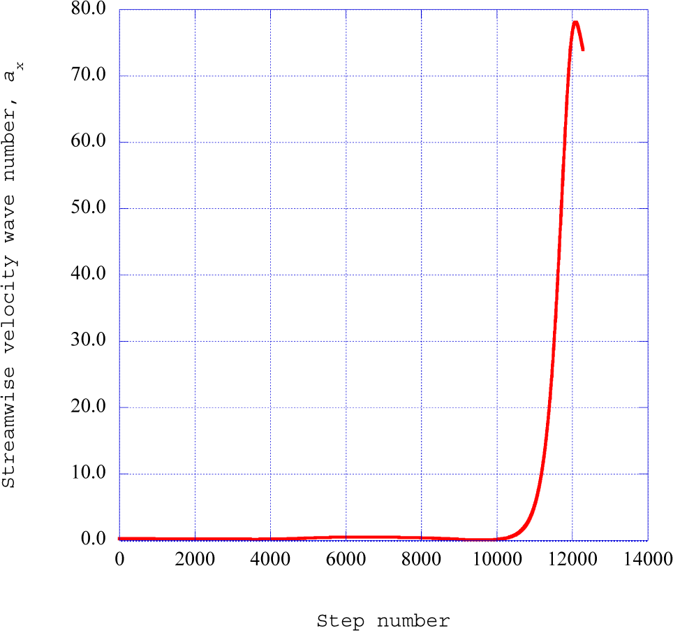
Figure 2 presents the fluctuating streamwise velocity wave components over the total time range of the integration process.
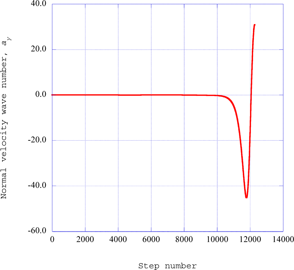
Figure 3 shows the corresponding normal velocity wave components over the same time frame.
Mathieu and Scott [
28] (pp. 239–282) have presented a thorough discussion of the method of spectral analysis applied to turbulent flow, involving both the spectral wave number components and the spectral velocity wave components. We should note that we have not restricted the solutions for the wave number components, but have simply transferred the resulting time series solutions to disk for retrieval in the solution of the time dependent velocity wave component equations,
Equations (26)–
(28). Also, an essential aspect of our computational procedure in the spectral plane is that the statistical analysis of the resulting time series solutions for the velocity wave components involves only the quadratic representations of these components to obtain the statistical properties of interest. Thomas [
30] presents an extensive discussion, including a number of definitions and propositions, regarding the use of Parseval’s theorem to show the identity between the quadratic form of the spectral velocity wave components and the quadratic form of the corresponding velocity fluctuations. We have therefore assigned the results of the statistical analysis of the quadratic spectral velocity wave components to the kinetic energy content of the corresponding physical fluctuating velocity components. This allows us to carry our computational procedure to the dissipation of kinetic energy into background thermal energy, representing the increase in thermal entropy.
5. Power Spectral Density Within the Deterministic Structure
The time series solutions for the spectral wave number components and the spectral velocity wave components indicate that after an induction period, a sharp instability occurs in the solutions. We classify this instability as a deterministic boundary layer structure. To obtain the entropy generation rate through this deterministic structure, it is necessary to extract the underlying structural characteristics of the nonlinear time series solutions. Chen [
18] has presented a series of studies of methods for the extraction of such structural information from time series information. A computer source code has been presented in [
20] that implements the maximum entropy method (Burg’s method) for spectral analysis of geophysical seismic time data records. This method considerably improves the spectral resolution of the power spectral density for short time series records.
Burg’s method has its theoretical roots in information theory (Cover and Thomas [
19]), where a discussion and a proof of Burg’s maximum entropy rate theorem are given. These authors also make reference to the work of Rissanen [
20,
21], where the maximum entropy method is related to the concept of Kolmogorov complexity [
22].
One of the significant advantages of Burg’s method is the enhancement of the spectral peaks in the power spectral density distribution. Our previous experience with Burg’s method and the existence of useful source codes for the analysis of the predicted time series led to our use of this method for the evaluation of the power spectral density of the streamwise velocity wave vector, ax, for each segment in the time series.
Press
et al. [
29] (pp. 572–575) present computer source codes for the prediction of the power spectral density using the maximum entropy method. The power spectral density for the streamwise velocity wave component time series is computed for 1024 time step data samples from time step of 11,264 to time step 12,288. The selected time series is divided into 32 segments with 32 data sets per segment. Burg’s method [
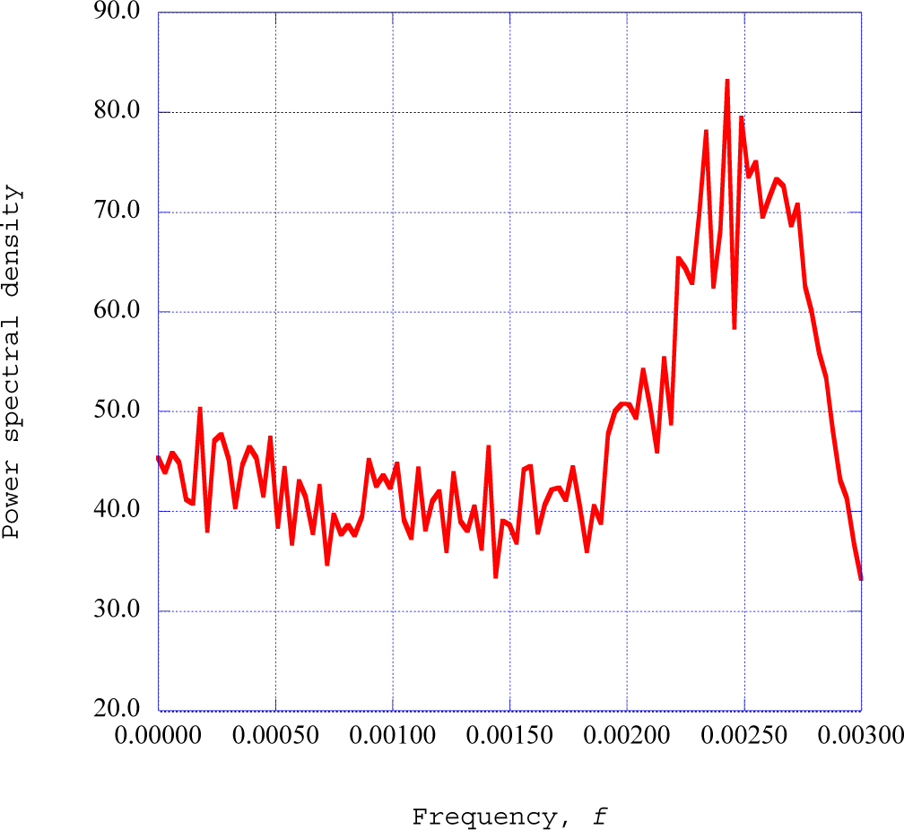
29] is then applied to each segment of the 32 data sets to obtain 16 spiked values of the power spectral density of the streamwise velocity wave component over the selected time series. The resulting power spectral density results for the deterministic structure for the conditions listed in
Table 1 are presented in
Figure 4.
The results shown in
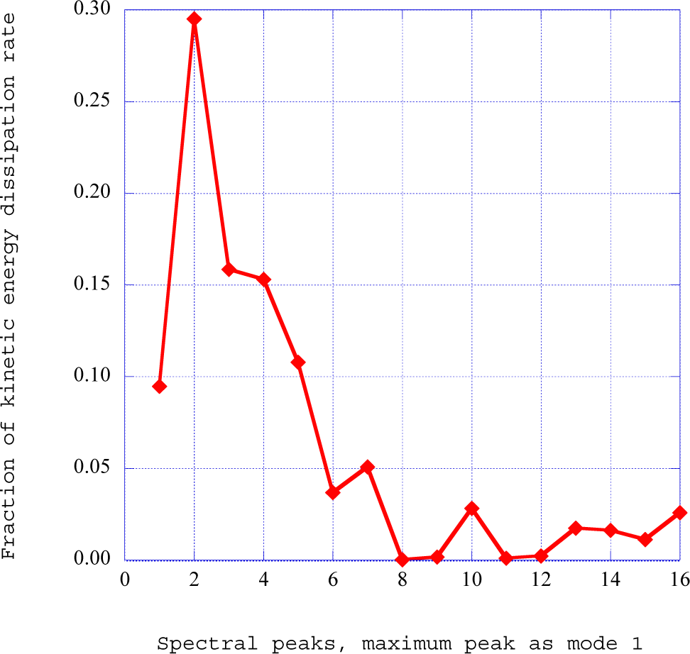
Figure 4 for the power spectral density indicate that the spectral energy is distributed in well-defined spectral peaks. We speculate at this point that the distribution of the kinetic energy available for dissipation is spread across these spectral peaks. We, therefore, number the “modes”, starting with the maximum peak as mode 1, numbering the peaks in decreasing amplitude to mode 16. We determine the kinetic energy dissipation rate [
28] for each mode with the relation:
The graphing program uses the trapezoidal rule to calculate the kinetic energy dissipation rate for each of the indicated peaks or modes. The total spectral energy dissipation rate is then obtained as the sum of the individual contributions across the modes.
Figure 5 shows the distribution of the fraction of total available kinetic energy dissipation rate across the sequence of peaks or modes in the power spectral density distribution shown in
Figure 4. The relatively low level indicated in mode 1 is apparently due to the narrow frequency range used in the integration process for the kinetic energy dissipation rate. In the development of a computational procedure for the determination of the entropy generation through the deterministic structure, we need to evaluate how much of the total kinetic energy dissipation rate in these modes actually contributes to the background thermal energy by dissipation within the deterministic structure. In the next section, we described the singular value decomposition process as a means to obtain a deeper definition of the underlying spectral characteristics of the time series solution found for the deterministic structure previously described.
6. Singular Value Decomposition and Empirical Entropy
Holmes
et al. [
23] have developed the method of proper orthogonal decomposition, or singular value decomposition, as a means of identifying additional characteristics of the nonlinear time series solutions for coupled, nonlinear flow equations. With the results from a direct numerical simulation of flow field structures serving as input data, these methods yield useful information concerning the distribution of fluctuating kinetic energy across coherent structures within the flow. We have incorporated into our numerical procedure singular value decomposition computer source codes presented by Press
et al. [
29] (pp. 59–65).
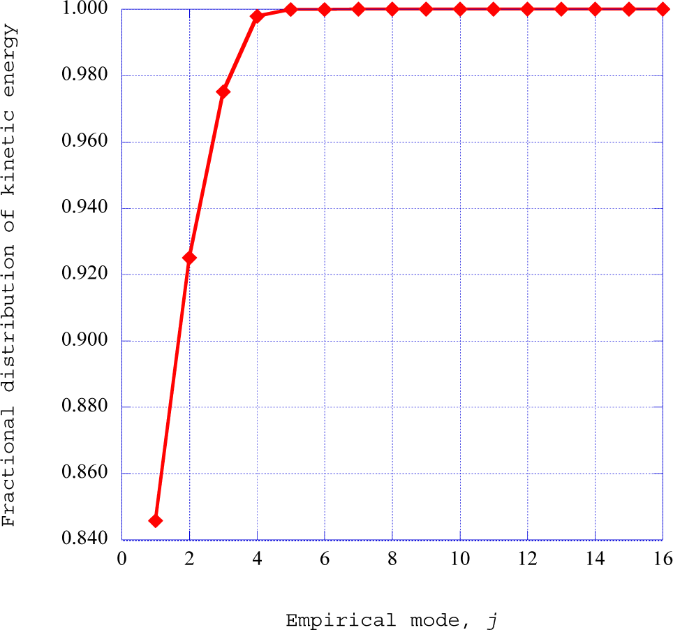
Figure 6 shows the fraction of kinetic energy in each of the empirical modes predicted by the application of the singular value decomposition to a selected time frame of the nonlinear time series for the streamwise velocity wave component.
The singular value decomposition computational procedure is made up of two parts, the computation of the autocorrelation matrix and the singular value decomposition of that matrix [
28]. The computation of the autocorrelation of the fluctuating streamwise velocity wave components is accomplished with the source code presented by Press
et al. [
29] (pp. 545–546). The source code presented by Press
et al. [
29] (pp. 66–70) for the computation of the singular value decomposition procedure, is also included in the computational process. This computational procedure yields the empirical eigenvalues for each of the empirical eigen functions for the given time series data segment.
The application of the singular value decomposition procedure to a specified segment of the nonlinear time-series solution for the streamwise velocity wave component yields the distribution of the component eigenvalues
λj across the empirical modes,
j, for the flow conditions listed in
Table 1. The empirical entropy,
Sempj, is defined from these eigenvalues by the expression (Rissanen [
20,
21]):
The singular value decomposition procedure for a specified segment of the nonlinear time-series solution yields the various eigenvalues
λj across the empirical modes,
j for the given segment [
9]. The particular empirical entropy of a particular mode
j provides an indication of the nature of the directed kinetic energy that exists within that particular mode.
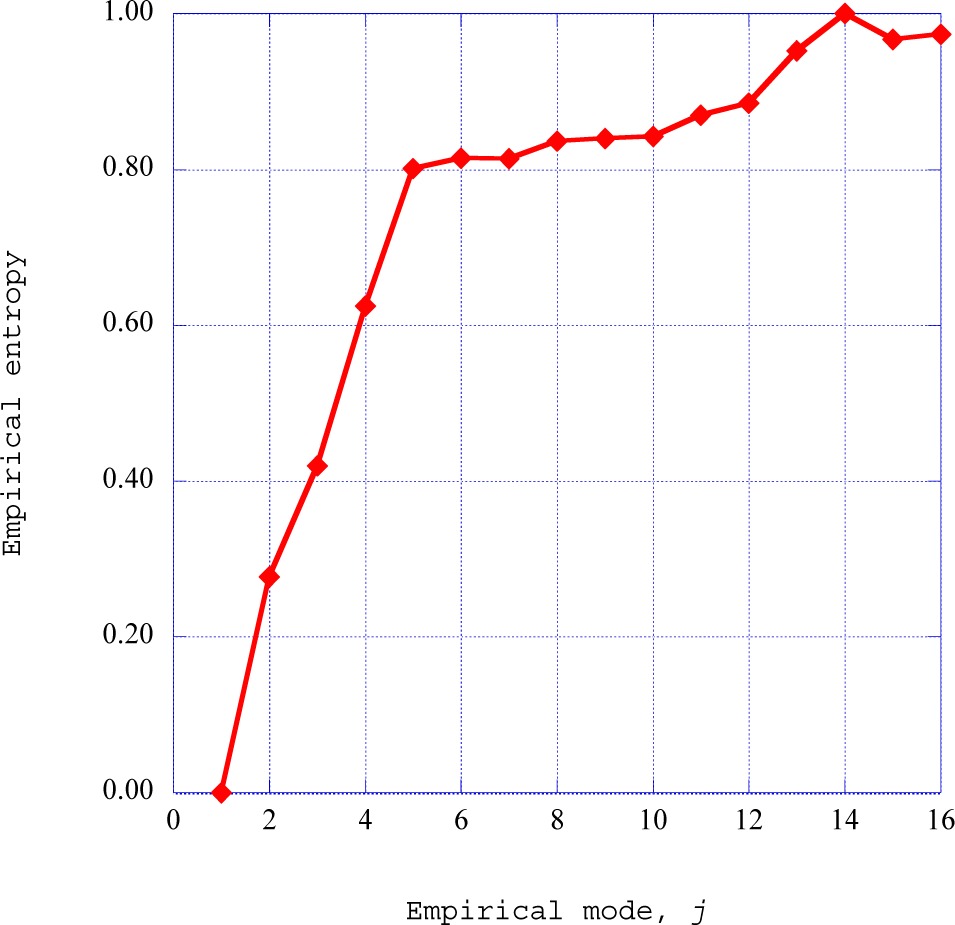
The empirical entropies for each of the empirical modes from one to sixteen for streamwise station x = 0.08 are shown in
Figure 7. The distribution of the empirical entropy over the empirical modes indicates three different characteristics for the nature of kinetic energy within the modes (Isaacson [
31]). The initial three eigenmodes contain relatively low levels of empirical entropy, indicating highly ordered directed kinetic energy. The following two modes indicate a steep increase in value, indicating a sharp increase in disorder within the kinetic energy environment. The following eleven modes indicate disordered kinetic energy, with the empirical entropy approaching the maximum of unity in value.
The interpretation we make for the eigenvalues
λj is that they represent twice the kinetic energy within each eigenmode distributed across
j values [
23]. These eigenmodes are obtained for the streamwise velocity wave components across a specified set of time series data, taken as a total ensemble of data values, and not as a
sequence of values. Thus, these empirical entropy values exist as a collection of values within the nonlinear time series, and not as a cascade from low entropy modes to high entropy modes. The computation of the empirical entropy has thus provided additional insight into the thermodynamic nature of our nonlinear time series solutions. We have, thus far, demonstrated the production of instabilities at a particular vertical station within a three-dimensional laminar boundary layer as a result of nonlinear interactions within the boundary layer. The empirical entropy further characterizes the nonlinear time series into regions of low empirical entropy, a transition region, and an extensive region of high empirical entropy, coexisting simultaneously within the time series solutions.
We wish to now explore some speculative thermodynamic concepts that allow us to extend our computational procedure through the deterministic structures produced by the instability process to a connection with the entropy generation rate produced in the final stage of the decay of the deterministic structure. These exploratory concepts are the empirical entropic index, the empirical intermittency exponent and the final entropy generation rate expression.
7. Empirical Entropic Index for Deterministic Structures
The empirical entropy for the fluctuating streamwise velocity wave component time series indicates different characteristics for the various deterministic regions within the time series. These results indicate that the majority of the kinetic energy in the deterministic structures is contained within the first three or four empirical modes of the singular value decompositions, with relatively low empirical entropy. These structures have been classified as coherent [
23] with well-defined structural boundaries. To characterize these structures, Tsallis [
24] postulated a generalized entropic form
In this expression, k is a positive constant, pi is the probability of the subsystem to be in the state i, and W is the total number of microscopic possibilities of the system. The Tsallis entropic index, q, would be found from this expression for an ensemble of accessible microscopic subsystems.
It is tempting to apply this expression for the ordered structures as calculated in the previous section on empirical entropy. However, the Tsallis entropic form is applicable to an ensemble of microscopic subsystems, while we are working with a set of individual macroscopic systems spread over a limited number of empirical modes,
j. In fact, the premise of the computation of the empirical entropy,
Sempj is that this is the entropy of an ordered region described by the empirical eigenvalue,
λj, for the singular value decomposition empirical mode,
j. Hence, we simply adopt, in an
ad hoc fashion, an expression from which we may extract an empirical index,
qj, from the empirical entropy. This expression may be written as:
We have to keep in mind that this expression does not have a mathematical basis in non-extensive thermo-statistics but is simply an artifact that allows us to include the effects of the nonlinear, non-equilibrium nature of the deterministic structures we are following. The expression has the format of entropic index; hence, we simply call it an empirical entropic index or simply an entropic index. We have used this expression to extract the empirical entropic index,
qj, from the empirical entropy for streamwise stations x = 0.08.
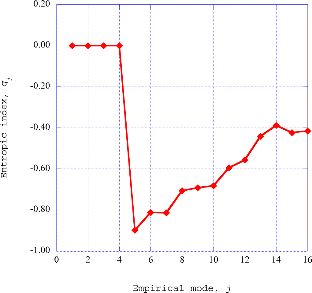
Figure 8 shows the empirical entropic indices for the streamwise velocity wave components at this station as a function of the empirical mode. The empirical entropic indices for empirical modes one through four indicate a zero value. Mariz [
25], indicates that for an entropic index of zero value,
dSempj/
dt = 0. These modes thus contain a high fraction of directed kinetic energy, flowing in the streamwise direction in a reversible and adiabatic process.
Glandsdorff and Prigogine [
26] find that for the general evolution criterion for non-equilibrium dissipative processes,
dSempj/
dt < 0. When the Tsallis entropic index is negative, Mariz [
25] found that the empirical entropy change is also negative,
dSempj/
dt < 0. The results presented in
Figure 8 indicate that significant deterministic structures exist within the specified time frame of the nonlinear time series solution. These regions may therefore be classified as ordered, dissipative structures. Therefore, the significant negative nature for the extracted empirical entropic indices from empirical modes five to sixteen at the streamwise station x = 0.08 is in agreement with both the Prigogine criterion and the Mariz results for the Tsallis entropic index. The
ad hoc introduction of an empirical entropy index may thus provide a representation of the nonlinear, non-equilibrium structures in a significant way.
8. Intermittency Exponents for Deterministic Structures
In this section, we introduce a speculative method to connect the deterministic results for the entropic indices with the turbulent dissipation processes occurring in the downstream fully developed turbulent flow. We explore this computational connection through the concept of turbulent intermittency.
The concept of intermittency arises in the observation that within a fully developed turbulent flow, regions of the dissipation of kinetic energy are interspersed with regions in which the dissipation rate is very low, with the regions separated by distinct boundary surfaces. This observation led to the characterization of the dissipation of turbulent kinetic energy in the inertial range as fractal in nature (Tsallis [
24]). Mathieu and Scott [
28] also present a thorough discussion of intermittency in the dissipation of turbulent kinetic energy within fully developed turbulent flows.
The deterministic structures discussed in previous sections are of a macroscopic nature embedded within the nonlinear time series solution of the nonlinear equations for the fluctuating velocity field. We have found, through the singular value decomposition method, that the four lowest empirical modes contain nearly 99 per cent of the kinetic energy. We have also found that the empirical modes obtained from the singular value decomposition indicate empirical entropic indices. We will therefore, heuristically, apply a relationship, found by Arimitsu and Arimitsu [
27], between the entropic index of Tsallis and the intermittency exponent required to account for the fractal nature of turbulent energy dissipation. We will substitute the absolute value of the empirical entropic index discussed in the previous section into the original derivation by Arimitsu and Arimitsu [
27]. This expression is written as:
Given the absolute value of the empirical entropic index,
qj, the intermittency exponent,
ζj for the mode,
j, is extracted from this expression by the use of Brent’s method [
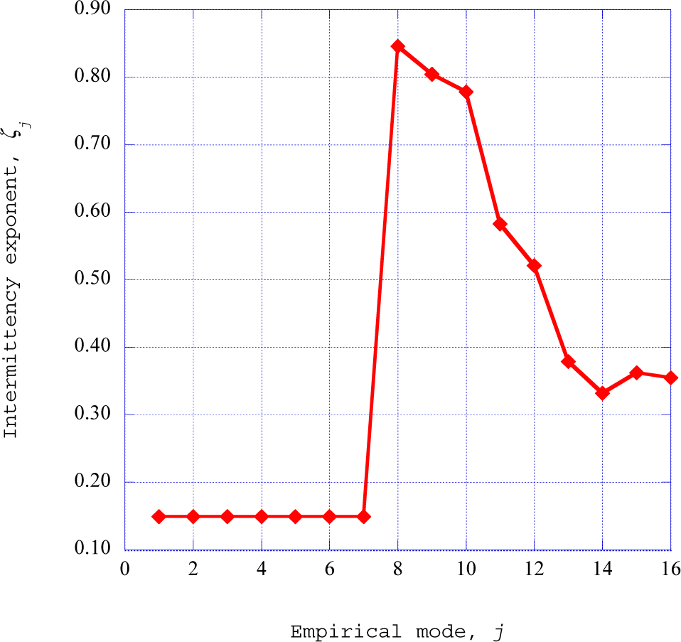
29] (pp. 397–405). The intermittency exponent is shown in
Figure 9 as a function of empirical mode,
j. Arimitsu and Arimitsu [
27] derive the intermittency exponents for turbulent eddies that dissipate turbulent kinetic energy into thermal energy within the flow.
9. Entropy Generation Rate through the Deterministic Boundary-Layer Structures
The fundamental need to improve the efficiency of thermal systems has sparked considerable effort to understand and reduce the generation of entropy in these systems. Recent studies (Ghasemi
et al. [
32,
33]) have computationally explored the entropy generation in transitional boundary layers subjected to various imposed free stream conditions. In Reference [
32], the effect of free-stream turbulence in the production of bypass transition was studied for the resulting generation of entropy within the boundary layer. Various computational methods were employed to gain a better understanding of the mechanisms involved in the generation of entropy within the boundary layer flows. Reference [
33] reports the results of the study of the effects of favorable and unfavorable pressure gradients imposed on the boundary layer in the generation of entropy within the boundary layer. Again, various computational methods were employed to obtain the extensive results.
An essential observation is presented in these studies. In Reference [
33], the imposition of external turbulence induces a “bypass” or early transition to turbulent flow. Experiments have indicated that transition is initiated by a primary instability mechanism in which a fundamental understanding is still lacking, thus hindering our understanding of entropy generation phenomena [
33]. The essential objective of the study reported here is to provide additional insight into possible mechanisms leading to the generation of deterministic structures within boundary-layer flows and the mechanisms by which entropy is generated through these structures.
At this point, we are ready to evaluate the entropy generation rate through the deterministic structures produced by the nonlinear interactions within the three-dimensional laminar boundary layer. To review what we have accomplished, we note that we have the local flow kinetic energy at the normalized vertical distance in the boundary layer that indicates the production of the initial instabilities. Through the power spectral density of the nonlinear fluctuating streamwise velocity wave component, we have the kinetic energy dissipation rate within each of the indicated peaks in the spectral distribution of the kinetic energy. The singular value decomposition procedure applied to the nonlinear time series solution for the streamwise velocity wave component yields a distribution of empirical entropic indices across a range of empirical mode numbers. Then, from these entropic indices, we have extracted corresponding empirical intermittency exponents for the range of empirical modes. Thus, we have calculated the input energy source for the deterministic structure, the distribution of the dissipation rates of the energy across the empirical modes of the spectral distribution within the deterministic structure, and the fraction of the energy in each of these empirical modes that dissipates into background thermal energy, thus increasing the entropy.
The entropy generation rate for an internal relaxation process from the Gibbs equation of thermodynamics may be written (de Groot and Mazur [
34])
In this expression,
s is the entropy per unit mass,
μ is the mechanical potential for the dissipation of the ordered structures into background thermal energy and
J(x) is the net source of the dissipation rates for the ordered kinetic energy available for dissipation. The kinetic energy initially applied to the deterministic structure is u
2/2 while the kinetic energy dissipation rate finally available is that found from the summation of the fraction of kinetic energy dissipation rate in each empirical mode,
ξj times the intermittency exponent for that mode,
ζj [
27]. We consider the dissipation of the ordered structures into background thermal energy as a relaxation process of the streamwise velocity in the initial state to the final equilibrium state of the streamwise velocity over the internal parameter x. The expression for the entropy generation rate may then be written as:
The boundary layer mean velocity may be written, from
Equation (7), as
u =
uef′ and the streamwise Mach number is given by:
At the final equilibrium state, the streamwise velocity of the dissipated structure vanishes. Substituting these expressions into
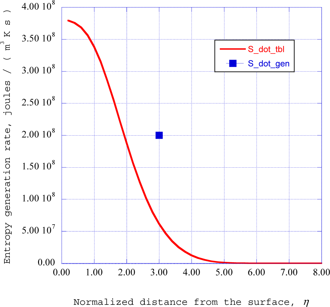
Equation (40), the entropy generation rate in energy per unit volume, temperature and time may be written as:
Substituting the results of the computational procedures as outline in the previous sections, the resulting value of the entropy generation rate is shown as a single point in
Figure 10.
For a comparison of this value of the entropy generation rate, we compute the entropy generation rate across a turbulent boundary layer for the given streamwise location. Following Truitt [
35] and Bejan [
36], the expression for the entropy generation rate in a turbulent boundary layer may be written, incorporating
Equation (4), as:
Applying the Falkner-Skan transformation,
Equation (5), in the differentiation with respect to y and the definition of the term:
the entropy generation rate across the turbulent boundary layer may be written as
The computation of the turbulent boundary layer begins at the initial streamwise station, at the initiation of the surface ripple, with transition enforced at that location. Hence, the turbulent boundary layer for our calculations at the streamwise location x = 0.08 is much smaller than a naturally occurring transition further along the streamwise direction. The distribution of the entropy generation rate across the turbulent boundary layer is shown in
Figure 10.
It is important to clarify why we have given only one data point in
Figure 10 for our computation of the rate of entropy generation through the deterministic structure within the instabilities in the laminar boundary layer. We emphasize that this is the value that is computed for the flow, thermodynamic, and transport properties given in
Table 1. We could change these values slightly and compute a new value for the entropy generation rate. We could then represent that value on
Figure 10. However, this becomes very misleading. Such a representation does not provide additional information concerning the validity of the procedure. The representation of additional data points could thus lead to a presumption of an inherent theoretical foundation that our exploratory computational procedure does not have. For example, a heuristic assumption is made in replacing the transfer matrix with a cosine function. Next, the empirical entropy function is heuristically constructed from the singular value decomposition results. Then, an entropic index form is extracted from these empirical entropy values with an artifact that simply yields reasonable computational values. The intermittency exponent for each of the empirical modes is obtained from an expression developed for fully consistent non-extensive entropic index values. Finally, the entropy generation rate is obtained from a non-equilibrium thermodynamic expression for the relaxation of an internal degree of freedom within an adiabatic system and is applied to the final dissipation of the ordered structure into background thermodynamic internal energy. Thus, the computational procedure has been constructed on a series of heuristic assumptions and some outright speculation. However, the computational results are encouraging and perhaps indicate some thread of truth in the computational procedure.
The thread we are seeking may possibly be found in the fabric of fractal-generated turbulent decay woven by the research group directed by Vassilicos [
37–
41]. In this research work, the decay of turbulence generated by low-blockage fractal square grids has been experimentally studied with a variety of fractal grids in several wind tunnel facilities. Of particular interest to us is the experimental result for the dissipation rate for fractal-generated turbulence [
38,
40], in which the turbulence dissipation rate has the same form as our
Equation (42). Thus, we have an independent experimental verification for our entropy generation rate results.
The flow through each of the square grids employed in the fractal-generated turbulence decay experiments has the same form as the flow through a short square duct. The developing boundary layers in the corners of a square duct develop secondary flows which appear as counter-rotating vortex structures [
4] (pp. 319–321). These developing boundary layers have the same three-dimensional nonlinear interactions that we have modeled in our computational procedure. For example, a Blasius boundary layer develops over the lower horizontal side of the square grid, with a velocity profile in the x-y plane. A similar Blasius boundary layer develops over the left-hand vertical side of the grid in the x-z plane. This boundary layer produces a velocity parallel to the lower horizontal side and in the positive z direction, acting normal to the x-y boundary layer profile. This three-dimensional nonlinear interaction produces deterministic structures in the boundary layer flow.
A corresponding effect occurs between the boundary layer produced in the x-z plane and a cross-flow velocity produced by the boundary layer flow in the x-y plane, thus producing a second deterministic structure in the corner three-dimensional boundary layer flow. The results for these nonlinear interactions are two, counter-rotating vortices, called secondary flow instabilities, occurring in each of the corners of the square fractal grids. Thus, our computational scenario should be applicable to this fractal flow environment, for the appropriate values of the thermodynamic and transport properties.
We have found in our research that dropping the pressure gradient contributions to the spectral equations for the velocity wave components,
Equations (17), yields a set of modified Burgers equations. The solution of these equations within the three-dimensional boundary-layer environment, with the steady boundary layer velocity gradients as control parameters, yields deterministic tightly wound spiral vortex structures. Application of this procedure to the corners of square ducts should then produce a pair of counter-rotating spiral vortices in each corner of the duct.
Our reference to the fractal-generated turbulence decay rate for validation of our entropy generation rate results has a direct relationship to our application of the computational scenario to the Richtmyer–Meshkov generated flow instabilities. The concept of the Tsallis entropic index [
24] is based in fractal concepts. We have introduced an empirical entropic index following these same concepts, but our index is simply an artifact that happens to yield numerical values for our given flow environment. Also, Arimitsu and Arimitsu [
27] developed the expression for the intermittency exponents that appear in our entropy generation rate expression through the consideration of turbulent dissipation of kinetic energy as a fractal process. Therefore, experimental results for the fractal-generated turbulence dissipation rate are of direct interest in the study reported here.
10. Discussion
The rippled surface of a foam substrate in a high power laser warm plasma experiment produces a strong oblique shock wave. It has been shown that such oblique shock waves produce a Richtmyer–Meshkov flow over the inclined substrate surface [
3]. We have developed a computational procedure to compute the development of boundary layer instabilities when a weak cross flow disturbance is applied to the boundary layer developed by the Richtmyer–Meshkov flow over the substrate surface [
3]. We have characterized these instabilities as a deterministic boundary layer structure. The computational procedure provides the power spectral density across a selected time frame within the deterministic structure [
11]. The rate of dissipation of kinetic energy within the narrow frequency range for each of the spectral peaks in the power spectrum has been computed [
28]. The kinetic energy at the given normalized vertical location in the boundary layer serves as the source of energy to the deterministic structure. The fraction of the dissipation rate of this total kinetic energy that is available in each of the modes within the deterministic structure is obtained from the power spectral density distribution across the selected time frame of the nonlinear time series. The method of singular value decomposition [
23] applied to a selected time frame of the time series solution yields values for the empirical entropy [
31] for a selected range of empirical modes. Empirical entropic indices [
31] are extracted from these empirical entropy values [
30]. Using results obtained from the fractal theory of turbulence dissipation [
27], the intermittency exponent is extracted for each of the empirical modes identified in the results of the singular value decomposition procedure. An essential aspect of the intermittency exponents is that these exponents represent the fraction of kinetic energy dissipation rate available in each empirical mode that is actually dissipated into background thermal energy of the flow [
26]. The product of the local boundary layer kinetic energy with the sum over the empirical modes of the fraction of the kinetic energy dissipation rate for each mode and the intermittency exponent for the corresponding mode represents the net dissipation rate for the kinetic energy within the deterministic structure that is actually transformed into background thermal energy.
From concepts of non-equilibrium thermodynamics [
31], we obtain an expression for the rate at which the flux of kinetic energy dissipation is converted into thermal energy. This rate turns out to be the global turnover rate as found in the experimental studies of fractal-generated turbulence decay [
38].
Thus, the entropy generation rate through a deterministic structure is found to be the product of the kinetic energy dissipation rate within the structure times the rate of relaxation along internal coordinates into background thermal energy divided by the local absolute temperature. Using the flow environmental parameters from
Table 1, the entropy generation rate is computed for warm dense plasma conditions. The resulting value is compared with entropy generation rates in a weak turbulent boundary layer [
33,
34] for these same input parameters and found to be comparable in value.


