Classification of Knee Joint Vibration Signals Using Bivariate Feature Distribution Estimation and Maximal Posterior Probability Decision Criterion

Abstract
:1. Introduction
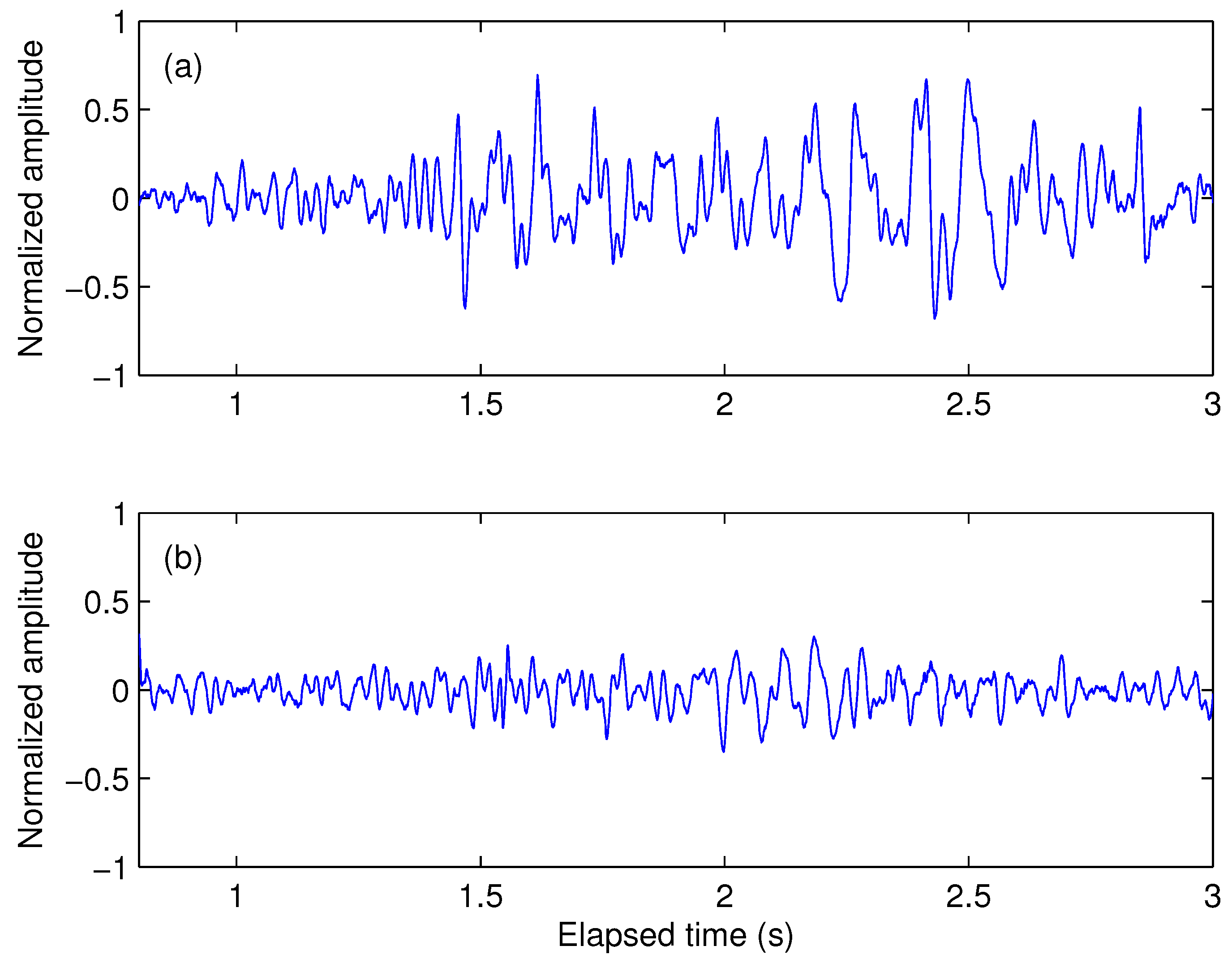
2. VAG Signal Acquisition and Feature Description
2.1. Dataset
2.2. Features Description
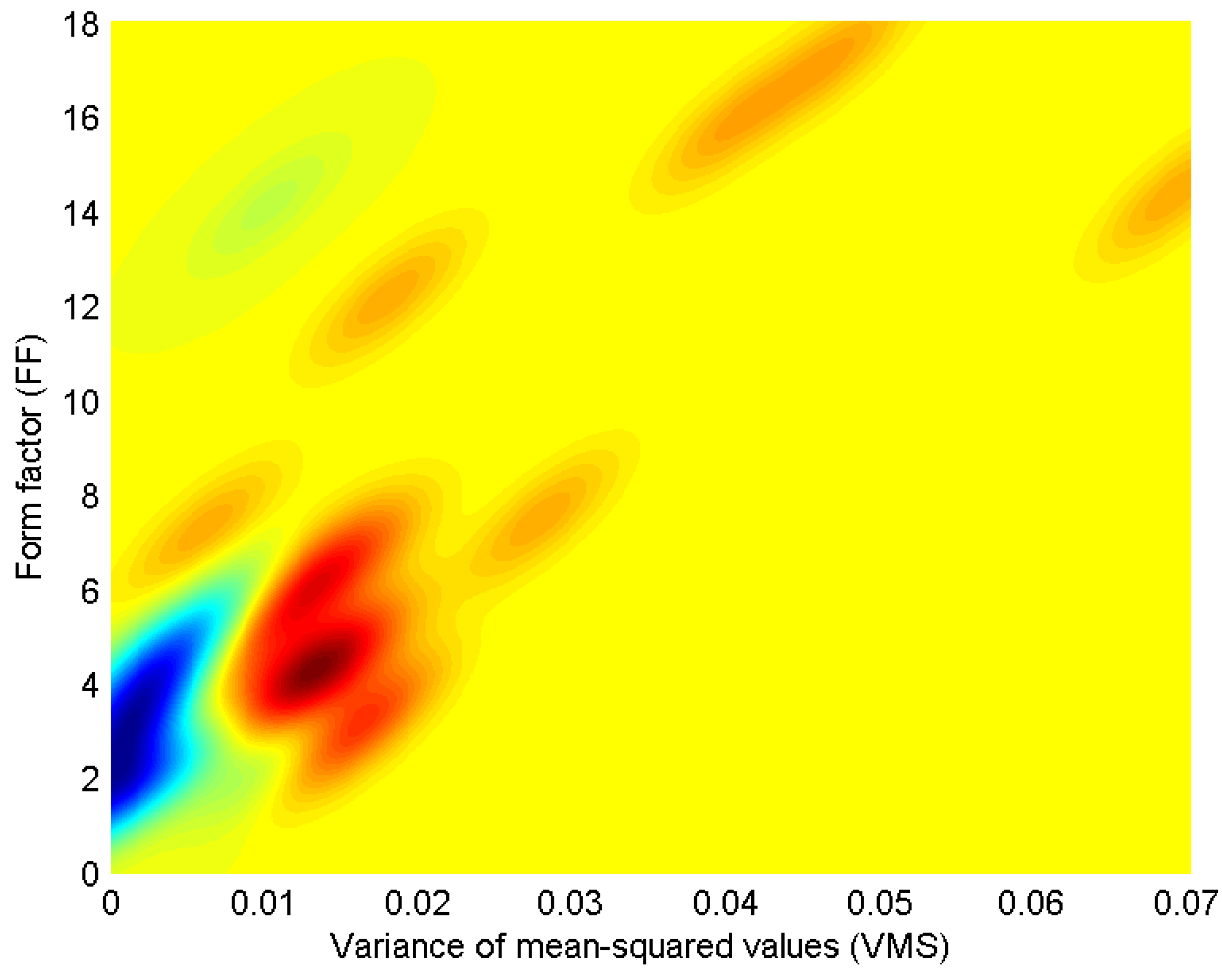
3. Bivariate Probability Distribution Modeling
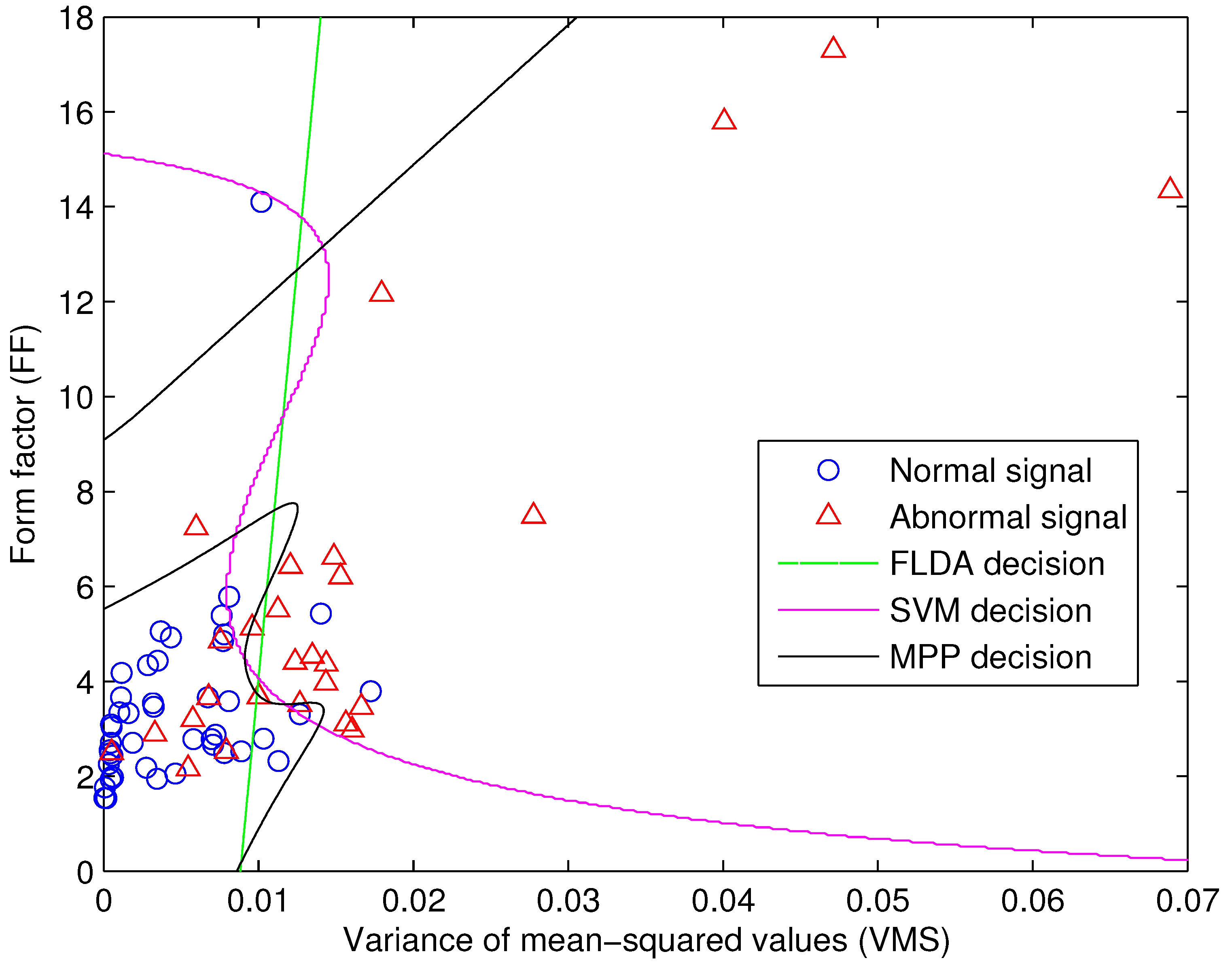
4. Signal Classification
4.1. Fisher’s Linear Discriminant Analysis
4.2. Maximal Posterior Probability Decision Criterion
4.3. Support Vector Machine
5. Results


| actual group | ||||
|---|---|---|---|---|
| Total number | positive | negative | ||
| 28 | 47 | |||
| classified group | positive | 24 | 19 | 5 |
| negative | 51 | 9 | 42 | |
| sensitivity | ||||
| specificity | ||||
| ± SE | ||||
| actual group | ||||
|---|---|---|---|---|
| Total number | positive | negative | ||
| 28 | 47 | |||
| classified group | positive | 25 | 18 | 7 |
| negative | 50 | 7 | 43 | |
| sensitivity | ||||
| specificity | ||||
| ± SE | ||||
| actual group | ||||
|---|---|---|---|---|
| Total number | positive | negative | ||
| 28 | 47 | |||
| classified group | positive | 27 | 21 | 6 |
| negative | 48 | 4 | 44 | |
| sensitivity | ||||
| specificity | ||||
| ± SE | ||||
6. Discussion and Conclusions
Acknowledgment
References
- Wu, Y.F.; Krishnan, S.; Rangayyan, R.M. Computer-aided diagnosis of knee-joint disorders via vibroarthrographic signal analysis: A review. Crit. Rev. Biomed. Eng. 2010, 38, 201–224. [Google Scholar] [PubMed]
- Vigorita, V.J. Orthopaedic Pathology; Lippincott Williams & Wilkins: Philadelphia, PA, USA, 1999. [Google Scholar]
- Frank, C.B.; Rangayyan, R.M.; Bell, G.D. Analysis of knee sound signals for non-invasive diagnosis of cartilage pathology. IEEE Eng. Med. Biol. Mag. 1990, 9, 65–68. [Google Scholar] [CrossRef] [PubMed]
- Manaster, B.J.; Crim, J.; Rosenberg, Z.S. Diagnostic and Surgical Imaging Anatomy: Knee, Ankle, Foot; Lippincott Williams & Wilkins: Philadelphia, PA, USA, 2007. [Google Scholar]
- Tanaka, N.; Hoshiyama, M. Vibroarthrography in patients with knee arthropathy. J. Back Musculoskelet. Rehabil. 2012, 25, 117–122. [Google Scholar] [PubMed]
- Jiang, C.C.; Lee, J.H.; Yuan, T.T. Vibration arthrometry in the patients with failed total knee replacement. IEEE Trans. Biomed. Eng. 2000, 47, 218–227. [Google Scholar]
- Reddy, N.P.; Rothschild, B.M.; Verrall, E.; Joshi, A. Noninvasive measurement of acceleration at the knee joint in patients with rheumatoid arthritis and spondyloarthropathy of the knee. Ann. Biomed. Eng. 2001, 29, 1106–1111. [Google Scholar] [CrossRef] [PubMed]
- Kim, K.S.; Seo, J.H.; Kang, J.U.; Song, C.G. An enhanced algorithm for knee joint sound classification using feature extraction based on time-frequency analysis. Comput. Methods Progr. Biomed. 2009, 94, 198–206. [Google Scholar] [CrossRef] [PubMed]
- Krishnan, S.; Rangayyan, R.M. Automatic de-noising of knee-joint vibration signals using adaptive time-frequency representations. Med. Biol. Eng. Comput. 2000, 38, 2–8. [Google Scholar] [CrossRef] [PubMed]
- Wu, Y.F.; Krishnan, S. Combining least-squares support vector machines for classification of biomedical signals: A case study with knee-joint vibroarthrographic signals. J. Exp. Theor. Artif. Intell. 2011, 23, 63–77. [Google Scholar] [CrossRef]
- Krishnan, S.; Rangayyan, R.M.; Bell, G.D.; Frank, C.B. Adaptive time-frequency analysis of knee joint vibroarthrographic signals for noninvasive screening of articular cartilage pathology. IEEE Trans. Biomed. Eng. 2000, 47, 773–783. [Google Scholar] [CrossRef] [PubMed]
- Rangayyan, R.M.; Wu, Y.F. Screening of knee-joint vibroarthrographic signals using statistical parameters and radial basis functions. Med. Biol. Eng. Comput. 2008, 46, 223–232. [Google Scholar] [CrossRef] [PubMed]
- Rangayyan, R.M.; Wu, Y.F. Analysis of vibroarthrographic signals with features related to signal variability and radial-basis functions. Ann. Biomed. Eng. 2009, 37, 156–163. [Google Scholar] [CrossRef] [PubMed]
- Rangayyan, R.M.; Oloumi, F.; Wu, Y.F.; Cai, S.X. Fractal analysis of knee-joint vibroarthrographic signals via power spectral analysis. Biomed. Signal Process. Control 2013, 8, 26–29. [Google Scholar] [CrossRef]
- Rangayyan, R.M.; Wu, Y.F. Screening of knee-joint vibroarthrographic signals using probability density functions estimated with Parzen windows. Biomed. Signal Process. Control 2010, 5, 53–58. [Google Scholar] [CrossRef]
- Rangayyan, R.M.; Krishman, S.; Bell, G.D.; Frank, C.B.; Ladly, K.O. Parametric representation and screening of knee joint vibroarthrographic signals. IEEE Trans. Biomed. Eng. 1997, 44, 1068–1074. [Google Scholar] [CrossRef] [PubMed]
- Umapathy, K.; Krishnan, S. Modified local discriminant bases algorithm and its application in analysis of human knee joint vibration signals. IEEE Trans. Biomed. Eng. 2006, 53, 517–523. [Google Scholar] [CrossRef] [PubMed]
- Cai, S.X.; Yang, S.S.; Zheng, F.; Lu, M.; Wu, Y.F.; Krishnan, S. Knee joint vibration signal analysis with matching pursuit decomposition and dynamic weighted classifier fusion. Comput. Math. Methods Med. 2013, 2013, 904267:1–904267:11. [Google Scholar] [CrossRef] [PubMed]
- Cai, S.X.; Wu, Y.F.; Xiang, N.; Zhong, Z.T.; He, J.; Shi, L.; Xu, F. Detrending Knee Joint Vibration Signals with a Cascade Moving Average Filter. In Proceedings of the 34th Annual International Conference of IEEE Engineering in Medicine and Biology Society (EMBC 2012), San Diego, CA, USA, 28 August–1 September 2012; pp. 4357–4360.
- Wu, Y.F.; Cai, S.X.; Lu, M.; Yang, S.S.; Zheng, F.; Xiang, N.; He, J.; Zhong, Z.T. Noise cancellation in knee joint vibration signals using a time-delay neural filter and signal power error minimization method. J. Converg. Inf. Technol. 2013, 8, 912–919. [Google Scholar]
- Rangayyan, R.M. Biomedical Signal Analysis: A Case-Study Approach; IEEE and Wiley: New York, NY, USA, 2002. [Google Scholar]
- Parzen, E. On estimation of a probability density function and mode. Ann. Math. Stat. 1962, 33, 1065–1076. [Google Scholar] [CrossRef]
- Xiang, N.; Cai, S.X.; Yang, S.S.; Zhong, Z.T.; Zheng, F.; He, J.; Wu, Y.F. Statistical analysis of gait maturation in children using nonparametric probability density function modeling. Entropy 2013, 15, 753–766. [Google Scholar] [CrossRef]
- Fisher, R.A. The use of multiple measurements in taxonomic problems. Ann. Eugen. 1936, 7, 179–188. [Google Scholar] [CrossRef]
- Jain, A.K.; Duin, R.P.W.; Mao, J.C. Statistical pattern recognition: A review. IEEE Trans. Pattern Anal. Mach. Intell. 2000, 22, 4–37. [Google Scholar] [CrossRef]
- Martinez, A.M.; Kak, A.C. PCA versus LDA. IEEE Trans. Pattern Anal. Mach. Intell. 2001, 23, 228–233. [Google Scholar] [CrossRef]
- Duda, R.O.; Hart, P.E.; Stork, D.G. Pattern Classification, 2nd ed.; Wiley: New York, NY, USA, 2001. [Google Scholar]
- Vapnik, V.N. Statistical Learning Theory; Wiley: New York, NY, USA, 1998. [Google Scholar]
- Cortes, C.; Vapnik, V.N. Support-vector networks. Mach. Learn. 1995, 20, 273–297. [Google Scholar] [CrossRef]
- Suykens, J.A.K.; van Gestel, T.; de Brabanter, J.; de Moor, B.; Vandewalle, J. Least Squares Support Vector Machines; World Scientific Publishing: Singapore, 2002. [Google Scholar]
© 2013 by the authors; licensee MDPI, Basel, Switzerland. This article is an open access article distributed under the terms and conditions of the Creative Commons Attribution license (http://creativecommons.org/licenses/by/3.0/).
Share and Cite
Wu, Y.; Cai, S.; Yang, S.; Zheng, F.; Xiang, N. Classification of Knee Joint Vibration Signals Using Bivariate Feature Distribution Estimation and Maximal Posterior Probability Decision Criterion. Entropy 2013, 15, 1375-1387. https://doi.org/10.3390/e15041375
Wu Y, Cai S, Yang S, Zheng F, Xiang N. Classification of Knee Joint Vibration Signals Using Bivariate Feature Distribution Estimation and Maximal Posterior Probability Decision Criterion. Entropy. 2013; 15(4):1375-1387. https://doi.org/10.3390/e15041375
Chicago/Turabian StyleWu, Yunfeng, Suxian Cai, Shanshan Yang, Fang Zheng, and Ning Xiang. 2013. "Classification of Knee Joint Vibration Signals Using Bivariate Feature Distribution Estimation and Maximal Posterior Probability Decision Criterion" Entropy 15, no. 4: 1375-1387. https://doi.org/10.3390/e15041375
APA StyleWu, Y., Cai, S., Yang, S., Zheng, F., & Xiang, N. (2013). Classification of Knee Joint Vibration Signals Using Bivariate Feature Distribution Estimation and Maximal Posterior Probability Decision Criterion. Entropy, 15(4), 1375-1387. https://doi.org/10.3390/e15041375