Article

Symmetry Properties of Bi-Normal and Bi-Gamma Receiver Operating Characteristic Curves are Described by Kullback-Leibler Divergences

by
Gareth Hughes
1,* and
Bhaskar Bhattacharya
2
1
Scotland's Rural College (SRUC), The King's Buildings, West Mains Road, Edinburgh EH9 3JG, UK
2
Department of Mathematics, Southern Illinois University, Carbondale, IL 62901-4408, USA
*
Author to whom correspondence should be addressed.
Entropy 2013, 15(4), 1342-1356; https://doi.org/10.3390/e15041342
Submission received: 26 February 2013 / Accepted: 2 April 2013 / Published: 10 April 2013

Abstract

:
Receiver operating characteristic (ROC) curves have application in analysis of the performance of diagnostic indicators used in the assessment of disease risk in clinical and veterinary medicine and in crop protection. For a binary indicator, an ROC curve summarizes the two distributions of risk scores obtained by retrospectively categorizing subjects as cases or controls using a gold standard. An ROC curve may be symmetric about the negative diagonal of the graphical plot, or skewed towards the left-hand axis or the upper axis of the plot. ROC curves with different symmetry properties may have the same area under the curve. Here, we characterize the symmetry properties of bi-Normal and bi-gamma ROC curves in terms of the Kullback-Leibler divergences (KLDs) between the case and control distributions of risk scores. The KLDs describe the known symmetry properties of bi-Normal ROC curves, and newly characterize the symmetry properties of constant-shape and constant-scale bi-gamma ROC curves. It is also of interest to note an application of KLDs where their asymmetry—often an inconvenience—has a useful interpretation.

1. Introduction

Receiver operating characteristic (ROC) curve analysis provides a basis for describing the performance of a diagnostic indicator when deployed in a binary diagnostic test. ROC curve analysis has found application in clinical medicine, veterinary medicine and crop protection (e.g., [1,2,3]). For a comprehensive overview of the methodology, see [4,5].
For the purpose of the present work, an outline description of the process by which an ROC curve may be derived allows us to introduce our terminology and notation. We refer generically to data provided by the diagnostic indicator as “risk scores”. During the process of characterizing a diagnostic indicator, a risk score is recorded for each of a number of experimental subjects. Each subject is also classified definitively as either a “case” (e.g., subject is diseased) or a “control” (e.g., subject is healthy) by a gold standard assessment (independent of the putative indicator). The ultimate goal of the experimental procedure as described is to provide a basis for decision-making in practice that does not require reference to the gold standard. When the decision in question is binary, an ROC curve is a useful summary of the performance of the diagnostic indicator [6].
We now have a number of subjects, and two values for each: a risk score provided by means of the diagnostic indicator and the true status (case or control) provided by the gold standard. We can present the results graphically as frequency distributions of risk scores plotted separately for cases and controls. It is normal practice to calibrate the output of the diagnostic indicator so that higher risk scores tend to be associated with case status, and lower risk scores tend to be associated with control status. Typically, then, the mean of the distribution of risk scores for cases is larger than the mean of the distribution of risk scores for controls.
An ROC curve is, in essence, a summary of the (normalized) frequency distributions of risk scores for cases and controls. In this article, we are concerned with the properties of ROC curves based on continuous parametric models for the distributions of risk scores (e.g., [5,7]). In practice, then, model parameters must be estimated from the experimental data; we do not describe this part of the analysis. For a continuous indicator variable X we refer to the resulting probability density functions (pdfs) as f1(x) (for cases) and f2(x) (for controls). The corresponding cumulative distribution functions (cdfs) are F1(x) and F2(x), respectively.
Now, consider the graphical plot of the pdfs of risk scores plotted separately for cases and controls. A diagnostic indicator and a threshold risk score together constitute a diagnostic test. In the process of developing a diagnostic test, our task is to characterize a threshold on the risk score scale such that subjects with risk scores above the threshold will be treated, and subjects with risk scores at or below the threshold will not be treated. The problem is that, typically, the distributions of risk scores for cases and controls overlap, so that there is no unequivocal “best” threshold risk score. Consider a particular choice of threshold risk score, and recall that we are working with the pdfs of risk scores for cases and controls. The proportion of cases correctly classified is the true positive proportion (TPP) and the proportion of controls correctly classified is the true negative proportion (TNP). The false negative proportion is FNP = 1 − TPP and the false positive proportion is FPP = 1 − TNP. The values of these proportions change with the choice of threshold risk score.
An ROC curve is a graphical plot of TPP [=1 − F1(x)] against FPP [=1 − F2(x)], with pairs of TPP and FPP values obtained by allowing a single threshold risk score to vary over the range of the indicator variable. Thus, points along the curve represent potential thresholds on the scale of the indicator variable, from each of which a binary test may be characterized. An ROC curve can therefore provide a useful summary of the characteristics of an indicator variable used as the basis for a binary test. Depending on the choice of model for risk scores for cases and controls, it may be possible to write down an analytical equation for the ROC curve, but this is immaterial in the present context. ROC curves that are monotone increasing above the main diagonal of the plot over the whole domain are sometimes referred to as “proper” ROC curves (see, e.g., Section 4.6 in [1]). Some continuous parametric ROC curves are proper, some are not; for example, it is well-known that the bi-Normal ROC curve is not in general proper, while the bi-gamma ROC curve is proper [8].
While on the one hand the ROC curve represents a summary of the distributions of risk scores for cases and controls, on the other there are methods by which a summary of the ROC curve itself is sought [7,9]. By far the most common single-figure ROC curve summary measure in use is the area under the curve (AUC) as an index of diagnostic accuracy (e.g., [10]). Briefly, the idea is that diagnostic indicators with ROC curves which pass close to the top left-hand corner of the graphical plot of TPP against FPP (high AUC) provide tests for which TPP and TNP are both high, offering good discrimination between cases and controls. Diagnostic indicators with ROC curves close to the main diagonal of the plot of TPP against FPP (low AUC) have little to offer in terms of discrimination between cases and controls. However, in the present context, the AUC is unsuitable for use in the description of the symmetry properties of ROC curves. It is not difficult to see that ROC curves with the same AUC may have different symmetry properties (e.g., Figure 2A in [11]; Figure 2 in [12]).
This article describes the symmetry properties of some parametric ROC curves based on continuous distributions. The article is set out as follows. The generic symmetry properties of ROC curves are described graphically. The application of the Kullback-Leibler divergence is outlined within the context of the present work. Some useful properties of the Pareto distribution are illustrated. The symmetry properties of bi-Normal, bi-exponential and bi-gamma ROC curves are analyzed. A general discussion is provided.

2. Analytical Background

2.1. Geometric Symmetry of ROC Curves

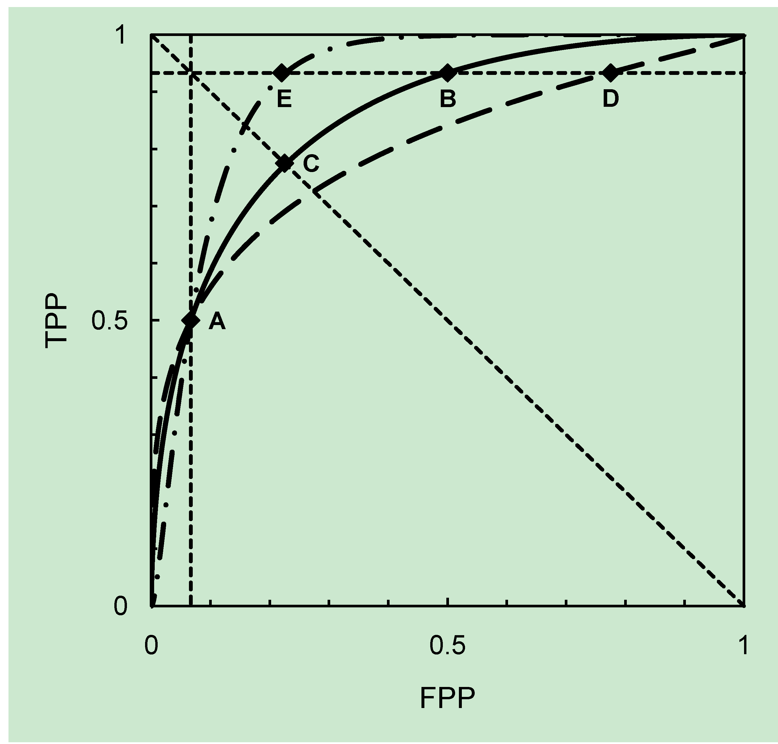
Geometric symmetry of ROC curves refers to an axis of symmetry that is the negative diagonal of the ROC plot (i.e., the line TPP = TNP). Green and Swets [13], Killeen and Taylor [14] and Hughes [15] have discussed the conditions for symmetry of ROC curves. However, ROC curves may be asymmetrical (skewed)—for example, the curve may “cling to the left edge of the ROC space longer than it does to the top” [16]. We refer to this kind of skew as TPP-asymmetry, and to the kind of skew where the curve clings to the top edge of the ROC space longer than it does to the left as TNP-asymmetry [17]. Figure 1 provides graphical definitions of these symmetry and asymmetry properties.
Figure 1. Graphical description of symmetric and asymmetric ROC curves. The dotted lines show, for reference, TPP = 1 − FPP (the negative diagonal) and the lines FPP = a (vertical) and TPP = 1 − a (horizontal). The FPP coordinate of point A = a, and the FPP coordinate of point C = a*, such that a < a*. The solid line is a symmetric ROC curve passing through the points A (a, b) and B (a1, b1) (such that a1 = 1 − b, b1 = 1 − a). Point C (a*, 1 − a*) also lies on the symmetric ROC curve. Asymmetries are defined by reference to the symmetric curve passing through point A, as follows. The dashed line is a TPP-asymmetric ROC curve passing through the points A (a, b) and D (a2, b2) (such that a2 > 1 − b, b2 = 1 − a). The dot-dashed line is a TNP-asymmetric ROC curve passing through the points A (a, b) and E (a3, b3) (such that a3 < 1 − b, b3 = 1 − a).
Entropy 15 01342 g001

2.2. Kullback-Leibler Divergences

For a continuous indicator variable X we denote pdfs f1(x) (for cases) and f2(x) (for controls). Then the Kullback-Leibler divergences (KLDs) [18] are I(f1,f2) (with cases as the comparison distribution and controls as the reference distribution):
I ( f 1 , f 2 ) = D f 1 ( x ) ln [ f 1 ( x ) f 2 ( x ) ] d x
and I(f2,f1) (with controls as the comparison distribution and cases as the reference distribution):
I ( f 2 , f 1 ) = D f 2 ( x ) ln [ f 2 ( x ) f 1 ( x ) ] d x
where D is the common support of f1 and f2.
From Cover and Thomas [19] (who refer to continuous KLDs as differential relative entropies) we note that I(f1,f2) and I(f2,f1) ≥ 0, with equality only if f1(x) and f2(x) are identical. Typically, I(f1,f2) ≠ I(f2,f1) [10] although for an ROC curve based on f1(x) (for cases) and f2(x) (for controls) that is symmetric about the negative diagonal, I(f1,f2) = I(f2,f1) [17]. A KLD can be interpreted as a kind of distance between probability distributions [19], although the asymmetry in its arguments (apart from some special cases) clearly indicates it is not a distance in the Euclidian sense. We will work in natural logarithms, so the KLDs are denominated in nits [20]. For a discussion of measures of distance between distributions as used in summarizing ROC curves, see Section 4.3.4 in [1].

2.3. The Pareto Distribution

Now, without for the moment invoking any ROC-related context, consider the Pareto densities:
f 1 ( x ) = 1 λ 1 ( x + 1 ) ( ( 1 / λ 1 ) + 1 )
f 2 ( x ) = 1 λ 2 ( x + 1 ) ( ( 1 / λ 2 ) + 1 )
x > 0 ; λ i > 0 , i = 1 , 2 . Following Ullah (Equation (3) in [21]) we obtain KLDs for two Pareto distributions, as follows:
I ( f 1 , f 2 ) = λ 1 λ 2 1 ln ( λ 1 λ 2 )
I ( f 2 , f 1 ) = λ 2 λ 1 1 ln ( λ 2 λ 1 ) .
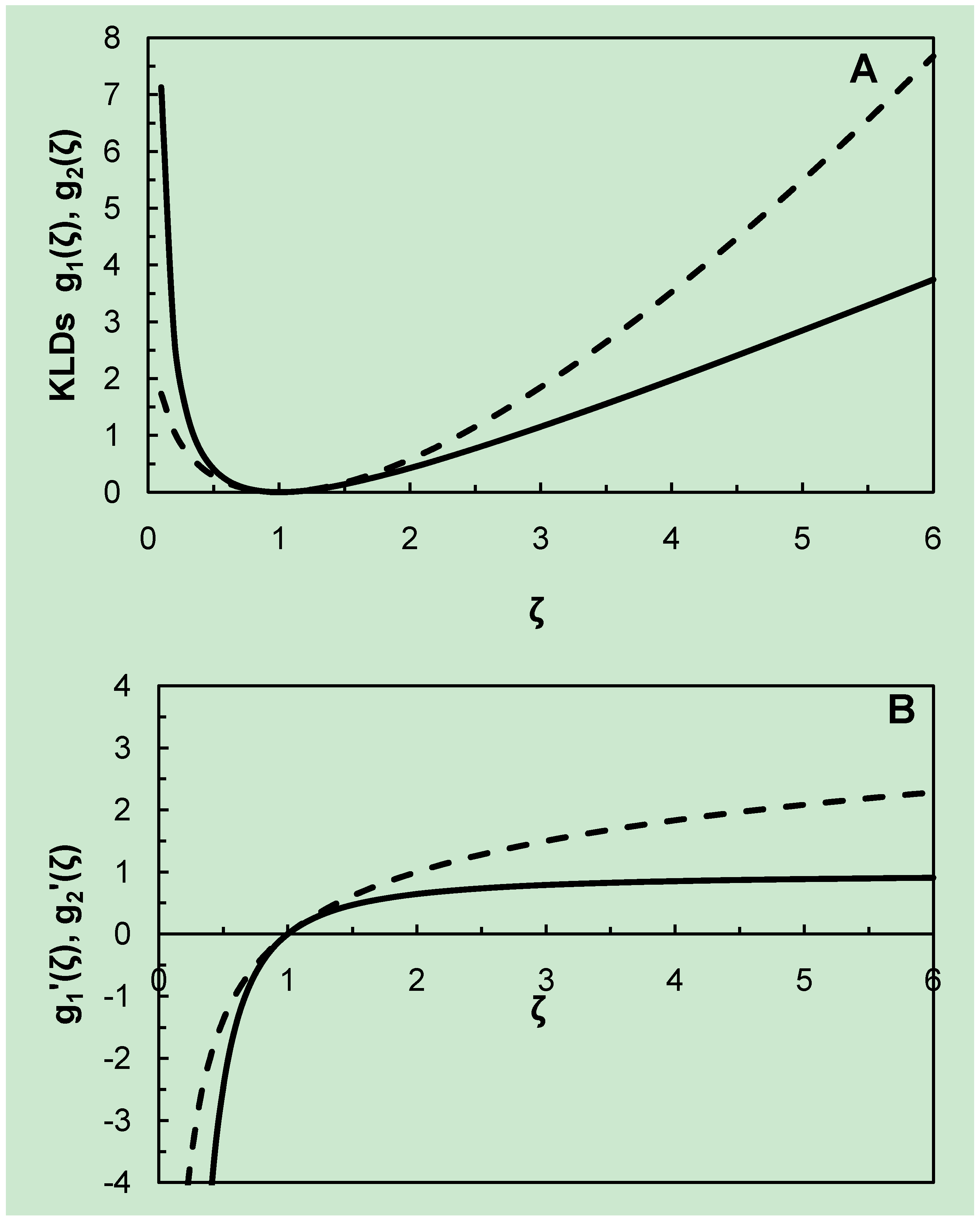
Let z = λ 2 / λ 1 ; since z 1 ln ( z ) with equality only if z = 1 (lemma 6.1 in [21]) we have both I(f1,f2) and I(f2,f1) ≥ 0, with equality only if f1(x) and f2(x) are identical (i.e., if λ 1 = λ 2 ), as required. Figure 2A shows the graphical plots of the two Pareto KLDs I ( f 1 , f 2 ) = g 1 ( z ) = 1 z 1 ln ( 1 z ) and I ( f 2 , f 1 ) = g 2 ( z ) = z 1 ln ( z ) , from which it appears that (for z > 0):
  • I ( f 1 , f 2 ) > I ( f 2 , f 1 ) when z < 1,
  • I ( f 1 , f 2 ) = I ( f 2 , f 1 ) when z = 1,
  • I ( f 1 , f 2 ) < I ( f 2 , f 1 ) when z > 1.
It turns out to be easier to characterize the inequality portrayed in Figure 2A if we calculate the derivatives g 1 / ( z ) = z 1 z 2 , g 2 / ( z ) = z 1 z . Now it is not difficult to see that for z > 0, g 2 / ( z ) g 1 / ( z ) with equality only if z = 1 (see also Figure 2B), and that this inequality describes the relationship between I(f1,f2) and I(f2,f1) shown in Figure 2. We will use these results on the Pareto distribution in the following sections.
Figure 2. (A). The figure shows graphical plots of Kullback-Leibler divergences for two Pareto densities: g 1 ( z ) = I ( f 1 , f 2 ) = ( 1 / z ) 1 ln ( 1 / z ) (the solid line), and g 2 ( z ) = I ( f 2 , f 1 ) = z 1 ln ( z ) (the dashed line), with z = λ 2 / λ 1 . (B). The derivatives g 1 / ( z ) = ( z 1 ) / z 2 (the solid line) and g 2 / ( z ) = ( z 1 ) / z (the dashed line).
Entropy 15 01342 g002

3. The Bi-Normal ROC Curve

For a continuous indicator variable X we have X ~ N ( μ 1 , σ 1 2 ) for cases and X ~ N ( μ 2 , σ 2 2 ) for controls, in which μ 1 and σ 1 2 denote the mean and variance, respectively, of f1(x); and μ 2 and σ 2 2 denote the mean and variance, respectively, of f2(x). The indicator variable is calibrated so that μ1 > μ2.
First we consider the symmetric bi-Normal ROC curve. For such curves, the standard deviations of the case and control distributions are equal, σ 1 = σ 2 [1]. Also, for symmetric ROC curves in general, the KLDs are equal I ( f 1 , f 2 ) = I ( f 2 , f 1 ) [17], and for the symmetric bi-Normal ROC curve in particular, I ( f 1 , f 2 ) = I ( f 2 , f 1 ) = ( μ 1 μ 2 ) 2 2 σ 2 ( > 0 ) ; σ 2 = σ 1 2 = σ 2 2 [23]. For a numerical example, consider Killeen and Taylor’s Figure 1 (top) in [14]. In this example, the distribution of risk scores for cases f1(x) is Normal with mean μ1 = 3.4 and standard deviation σ1 = 1 and the distribution of risk scores for controls f2(x) is Normal with mean μ2 = 2 and standard deviation σ2 = 1. The resulting ROC curve is geometrically symmetric [14] and I(f1,f2) = I(f2,f1) = 0.980 nits.
Asymmetric bi-Normal ROC curves are discussed by Green and Swets [13], Pepe [1] and Marzban [24]. In the terminology of the present article, bi-Normal ROC curves are TPP-asymmetric when σ 2 / σ 1 < 1 and TNP-asymmetric when σ 2 / σ 1 > 1 . Writing in the context of applications of bi-Normal indicators in clinical epidemiology, Pepe [1] notes that the distribution of risk scores for controls is typically less dispersed than the distribution of risk scores for cases, in which case a typical bi-Normal ROC curve would be TPP-asymmetric (e.g., Figure 4.1 in [1], where σ 2 / σ 1 = 0.85 ).
The KLDs are now (e.g., [15]):
I ( f 1 , f 2 ) = 1 2 [ σ 1 2 σ 2 2 1 ln ( σ 1 2 σ 2 2 ) + ( μ 1 μ 2 ) 2 σ 2 2 ]
I ( f 2 , f 1 ) = 1 2 [ σ 2 2 σ 1 2 1 ln ( σ 2 2 σ 1 2 ) + ( μ 1 μ 2 ) 2 σ 1 2 ] .
Let z = σ 2 2 σ 1 2 , and we can write these as:
I ( f 1 , f 2 ) = ( μ 1 μ 2 ) 2 2 σ 2 2 + 1 2 [ 1 z 1 ln ( 1 z ) ]
I ( f 2 , f 1 ) = ( μ 1 μ 2 ) 2 2 σ 1 2 + 1 2 [ z 1 ln ( z ) ] .
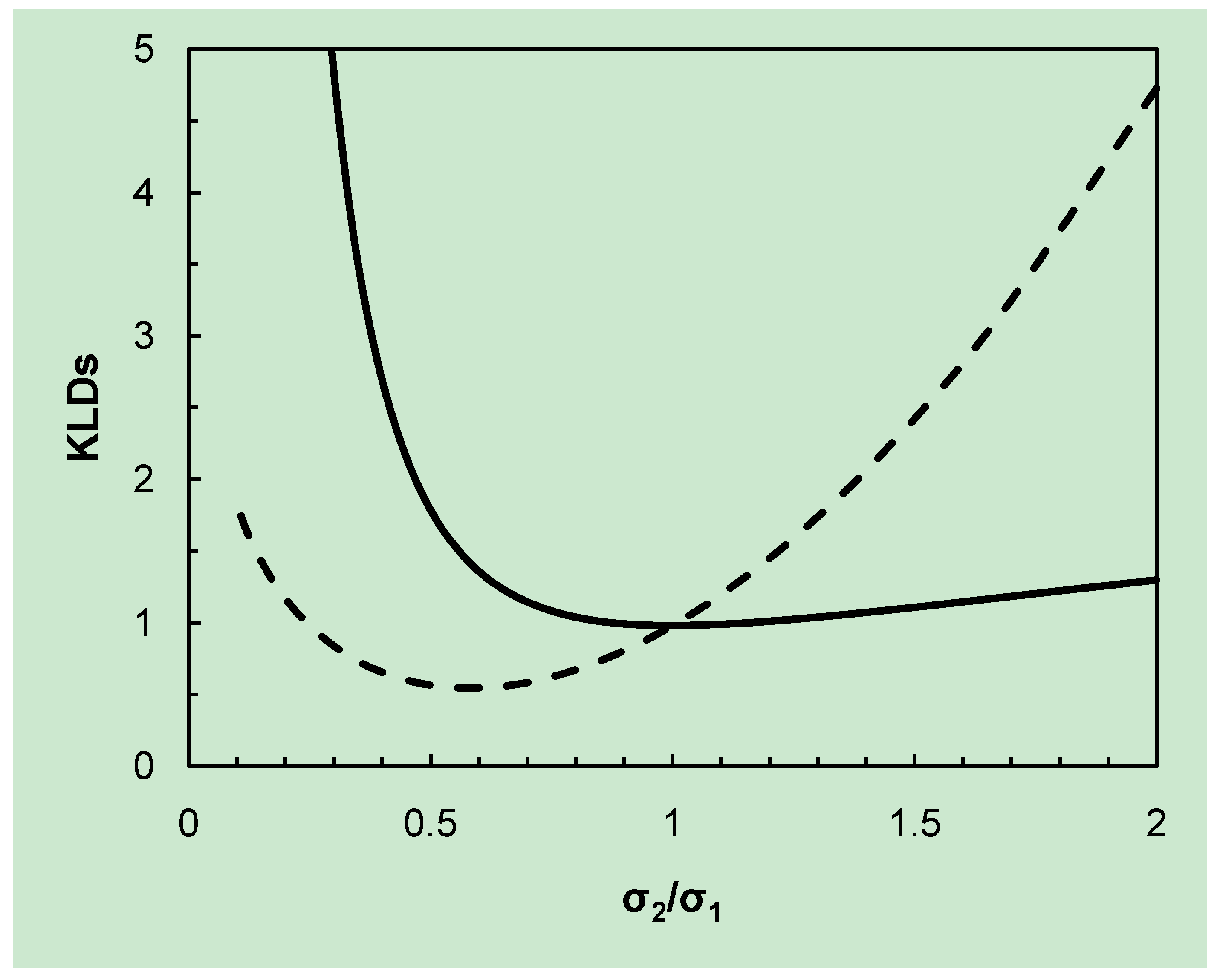
We compare this with the situation when σ 1 = σ 2 , I ( f 1 , f 2 ) = I ( f 2 , f 1 ) , and the ROC curve is symmetric. For TPP-asymmetry, we have σ 2 / σ 1 < 1 ; then ( μ 1 μ 2 ) 2 2 σ 2 2 > ( μ 1 μ 2 ) 2 2 σ 1 2 and (referring to Figure 2A) we can see that 1 2 [ 1 z 1 ln ( 1 z ) ] > 1 2 [ z 1 ln ( z ) ] . For TNP-asymmetry σ 2 / σ 1 > 1 ; then ( μ 1 μ 2 ) 2 2 σ 2 2 < ( μ 1 μ 2 ) 2 2 σ 1 2 and (referring again to Figure 2A) 1 2 [ 1 z 1 ln ( 1 z ) ] < 1 2 [ z 1 ln ( z ) ] . The inclusion of the factor ½ does not affect the inequality portrayed. Thus, for TPP-asymmetry, we have I ( f 1 , f 2 ) > I ( f 2 , f 1 ) and for TNP-asymmetry, we have I ( f 1 , f 2 ) < I ( f 2 , f 1 ) . This is illustrated in Figure 3, using values of μ1 and μ2 from Killeen and Taylor (Figure 1 in [14]). We note also from Figure 3 that the point where the two curves intersect characterizes the symmetric ROC curve with I(f1,f2) = I(f2,f1) = 0.980 nits.
Figure 3. Analysis of a bi-Normal ROC curve. The graph shows the Kullback-Leibler divergences I(f1,f2) (the solid line) and I(f2,f1) (the dashed line) for two Normal densities; f1(x) for cases has μ1 = 3.4 and σ1 is varied over a range that includes σ1 = 1, and f2(x) for controls has μ2 = 2.0 and σ2 = 1. When σ2/σ1 = 1, I(f1,f2) = I(f2,f1) and the corresponding ROC curve is symmetric about the negative diagonal. When σ2/σ1 < 1, I(f1,f2) > I(f2,f1) and the corresponding ROC curve is TPP-asymmetric; when σ2/σ1 > 1, I(f2,f1) > I(f1,f2) and the corresponding ROC curve is TNP-asymmetric.
Entropy 15 01342 g003

4. The Bi-Exponential ROC Curve

We deal with the bi-exponential ROC curve in passing, since it turns out to be a special case of the constant-shape bi-gamma ROC curve, below. Here, we have exponential densities for cases and controls (e.g., [25]), respectively:
f 1 ( x ) = 1 λ 1 exp ( x λ 1 )
f 2 ( x ) = 1 λ 2 exp ( x λ 2 )
x > 0 ; λ i > 0 , i = 1 , 2 . The indicator variable is calibrated so that the mean of the case distribution is larger than the mean of the control distribution, which requires λ 1 > λ 2 . A graphical plot of 1−F1(x) against 1−F2(x) then provides the ROC curve. Such ROC curves are TPP-asymmetric (as described in Figure 1) (see, e.g., Figure 1 in [25]).
Asadi et al. (Table 13.1 in [26]) provide a table of distributions related to the Pareto distribution by fixed transformation. Note that in the notation of Asadi et al. [26], our Pareto parameterization 1 λ i = β i , i = 1 , 2 . Then, following Asadi et al. [26], we obtain KLDs for two exponential distributions as follows:
I ( f 1 , f 2 ) = λ 1 λ 2 1 ln ( λ 1 λ 2 )
I ( f 2 , f 1 ) = λ 2 λ 1 1 ln ( λ 2 λ 1 ) .
Let z = λ 2 / λ 1 and refer to Figure 2A. For a useful ROC curve we require λ 1 > λ 2 , so we are only interested in the part of Figure 2A where z <1, and here we have I ( f 1 , f 2 ) > I ( f 2 , f 1 ) . For λ 1 = λ 2 , the case and control distributions are identical, I ( f 1 , f 2 ) = I ( f 2 , f 1 ) = 0 , and the corresponding ROC curve follows the main diagonal of the plot; such diagnostic indicators offer no discrimination between cases and controls.

5. The Bi-Gamma ROC Curve

We start by writing a general gamma density:
f ( x ) = x r 1 λ r Γ ( r ) exp ( x λ )
x > 0 ; r , λ > 0 . We refer to r as a shape parameter and λ as a scale parameter. Mathiassen et al. [27], Faraggi and Reiser [28], Faraggi et al. [29], and Hussain [30] use the same format. For two such gamma densities, respectively f1(x) and f2(x), we have X~gamma(x, r1, λ1) and X~gamma(x, r2, λ2) and the corresponding KLDs (e.g., [27]) are:
I ( f 1 , f 2 ) = ln ( Γ ( r 2 ) λ 2 r 2 Γ ( r 1 ) λ 1 r 1 ) + ( r 1 r 2 ) ( Ψ ( r 1 ) + ln ( λ 1 ) ) + r 1 ( λ 1 λ 2 1 )
I ( f 2 , f 1 ) = ln ( Γ ( r 1 ) λ 1 r 1 Γ ( r 2 ) λ 2 r 2 ) + ( r 2 r 1 ) ( Ψ ( r 2 ) + ln ( λ 2 ) ) + r 2 ( λ 2 λ 1 1 )
in which Γ(∙) is the gamma function and Ψ(∙) is the digamma function (the derivative of the logarithm of the gamma function, [31]). Here, we describe separately a constant-shape ROC curve and a constant-scale ROC curve.

5.1. The Constant-Shape Bi-Gamma ROC Curve

Here, r 1 = r 2 = r , 0 < r < ; λ 1 λ 2 > 0 . For f1(x) and f2(x) respectively, X~gamma(x, r, λ1) and X~gamma(x, r, λ2). The indicator variable is calibrated so that the mean of the case distribution is larger than the mean of the control distribution, which requires r λ 1 > r λ 2 . A graphical plot of 1−F1(x) against 1−F2(x) then provides the ROC curve. Such curves are TPP-asymmetric (as described in Figure 1). For example, see Dorfman et al. [8]. If r = 1, f1(x) and f2(x) are the same as for the bi-exponential ROC curve (above), and the symmetry properties then follow. Otherwise, the general gamma KLDs above simplify to:
I ( f 1 , f 2 ) = r [ λ 1 λ 2 1 ln ( λ 1 λ 2 ) ]
I ( f 2 , f 1 ) = r [ λ 2 λ 1 1 ln ( λ 2 λ 1 ) ]
and again, we can refer to Figure 2A (the inclusion of the (constant) factor r does not affect the inequality portrayed). For a useful ROC curve we require λ 1 > λ 2 , so we are only interested in the part of Figure 2A where z <1, and here we have I ( f 1 , f 2 ) > I ( f 2 , f 1 ) . For λ 1 = λ 2 , the case and control distributions are identical, I ( f 1 , f 2 ) = I ( f 2 , f 1 ) = 0 , and the corresponding ROC curve follows the main diagonal of the plot; such diagnostic indicators offer no discrimination between cases and controls.

5.2. The Constant-Scale Bi-Gamma ROC Curve

Here, r 1 r 2 > 0 ; λ 1 = λ 2 = λ > 0 . For simplicity, we follow Hanley [32] and Tang et al. [33] who have λ = 1. For f1(x) and f2(x) respectively, X~gamma(x, r1, λ) and X~gamma(x, r2, λ). The indicator variable is calibrated so that the mean of the case distribution is larger than the mean of the control distribution, which requires r 1 λ > r 2 λ . A graphical plot of 1−F1(x) against 1−F2(x) then provides the ROC curve. Such curves are TNP-asymmetric (as described in Figure 1). The general gamma KLDs above simplify to:
I ( f 1 , f 2 ) = ln ( Γ ( r 2 ) Γ ( r 1 ) ) + ( r 1 r 2 ) ( Ψ ( r 1 ) )
I ( f 2 , f 1 ) = ln ( Γ ( r 1 ) Γ ( r 2 ) ) + ( r 2 r 1 ) ( Ψ ( r 2 ) )
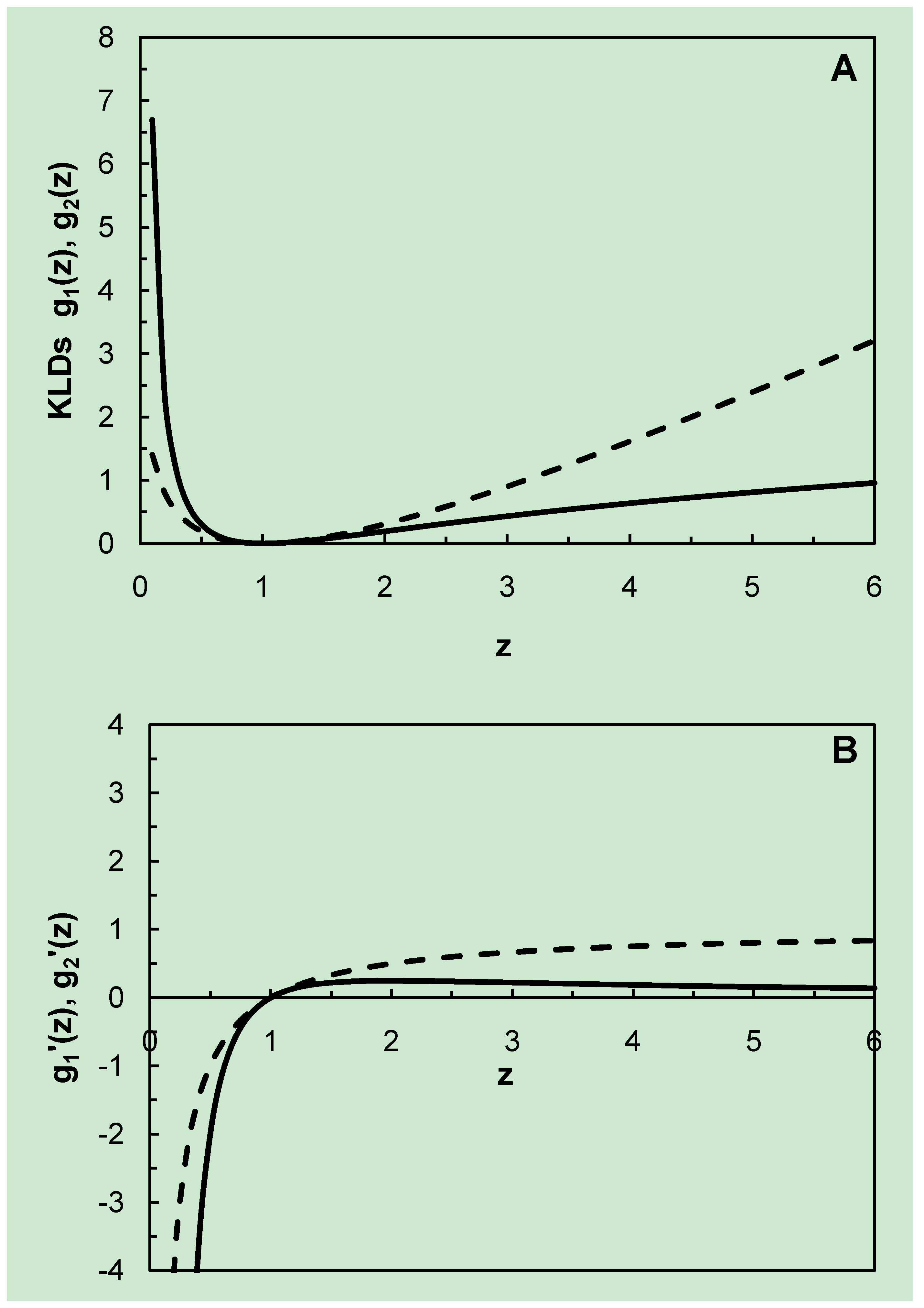
Now, we set r2 = 1 and r1 = ζ, ζ > 0. Figure 4A shows the graphical plots of:
  • I ( f 1 , f 2 ) = g 1 ( ζ ) = ln ( Γ ( ζ ) ) + ( ζ 1 ) Ψ ( ζ )
  • I ( f 2 , f 1 ) = g 2 ( ζ ) = ln ( Γ ( ζ ) ) + ( 1 ζ ) Ψ ( 1 )
from which it appears that (for ζ > 0):
  • I ( f 1 , f 2 ) > I ( f 2 , f 1 ) when ζ < 1,
  • I ( f 1 , f 2 ) = I ( f 2 , f 1 ) when ζ = 1,
  • I ( f 1 , f 2 ) < I ( f 2 , f 1 ) when ζ > 1.
On calculating the derivatives, g 1 / ( ζ ) = ( ζ 1 ) Ψ ( 1 ) ( ζ ) in which Ψ ( 1 ) ( ) is the trigamma function (the first derivative of the digamma function, [31]) and g 2 / ( ζ ) = Ψ ( ζ ) + γ in which γ is Euler’s constant (= 0.5772…) (see also Figure 4B). Recall that Ψ ( 1 ) = γ , then we have g 1 / ( 1 ) = g 2 / ( 1 ) = 0 , and the inequality portrayed in Figure 4 appears to have the same characteristics as that shown in Figure 2. Let g 3 ( ζ ) = g 2 / ( ζ ) g 1 / ( ζ ) = Ψ ( ζ ) + γ ( ζ 1 ) Ψ ( 1 ) ( ζ ) . Then the derivative g 3 / ( ζ ) = ( ζ 1 ) Ψ ( 2 ) ( ζ ) in which Ψ ( 2 ) ( ) is the tetragamma function (the second derivative of the digamma function, [31]). For ζ > 0 , Ψ ( 2 ) ( ζ ) is negative [31], so (for ζ > 0):
  • when ζ < 1, g 3 / ( ζ ) is negative and g 3 ( ζ ) = g 2 / ( ζ ) g 1 / ( ζ ) is decreasing,
  • when ζ = 1, g 3 / ( 1 ) is zero and g 3 ( ζ ) is stationary,
  • when ζ > 1, g 3 / ( ζ ) is positive and g 3 ( ζ ) is increasing,
which shows that for ζ > 0 , g 3 ( ζ ) 0 ; i.e., g 2 / ( ζ ) g 1 / ( ζ ) with equality only if ζ = 1. This inequality describes the relationship between I(f1,f2) and I(f2,f1) shown in Figure 4.
Figure 4. Analysis of a constant scale bi-gamma ROC curve. (A). Graphical plots of Kullback-Leibler divergences: g 1 ( ζ ) = I ( f 1 , f 2 ) = ln ( Γ ( ζ ) ) + ( ζ 1 ) Ψ ( ζ ) (the solid line), and g 2 ( ζ ) = I ( f 2 , f 1 ) = ln ( Γ ( ζ ) ) + ( 1 ζ ) Ψ ( 1 ) (the dashed line), with r2 = 1 and r1 = ζ, ζ > 0. (B). The derivatives g 1 / ( ζ ) = ( ζ 1 ) Ψ ( 1 ) ( ζ ) (the solid line) and g 2 / ( ζ ) = Ψ ( ζ ) + γ (the dashed line).
Entropy 15 01342 g004
For a useful ROC curve we require r 1 > r 2 , so we are only interested in the part of Figure 4A where ζ > 1, and here we have I ( f 1 , f 2 ) < I ( f 2 , f 1 ) . For r 1 = r 2 , the case and control distributions are identical, I ( f 1 , f 2 ) = I ( f 2 , f 1 ) = 0 , and the corresponding ROC curve follows the main diagonal of the plot; such diagnostic indicators offer no discrimination between cases and controls.

6. Discussion

For continuous parametric ROC curves, we can define symmetry conditions. Notwithstanding, it is sometimes rather difficult to tell from a graphical plot whether an empirical ROC curve is actually symmetrical or only approximately so (e.g., Figure 2 in [24]). It is harder to define asymmetry conditions for continuous parametric ROC curves, although often relatively easy to tell from a graphical plot when an empirical ROC curve is asymmetric (e.g., Figure 2 in [10]). Marzban [24] asks if asymmetry can be explained in terms of the underlying case and control distributions, and concludes that asymmetry in an ROC curve “can be attributed to unequal widths of the underlying distributions”. What is lacking is an independent assessment of asymmetry for comparison with the statistical assessment based on the relative dispersion of the case and control distributions. Here, we bring together a graphical definition of asymmetry (Figure 1) with an analysis of the KLDs for the case and control distributions for some examples of continuous parametric ROC curves.
The main findings are as follows. Bi-Normal ROC curves may be symmetric, TPP-asymmetric or TNP-asymmetric. For symmetric bi-Normal curves, we have I ( f 1 , f 2 ) = I ( f 2 , f 1 ) ; for TPP-asymmetric curves, I ( f 1 , f 2 ) > I ( f 2 , f 1 ) ; and for TNP-asymmetric curves, I ( f 1 , f 2 ) < I ( f 2 , f 1 ) . Of particular interest is the point of intersection of the two curves in Figure 3. The fact that at this point we have I ( f 1 , f 2 ) = I ( f 2 , f 1 ) > 0 indicates the existence of symmetric curves that lie above the main diagonal of the bi-Normal ROC plot. This in itself is not surprising, of course, but it is noted here for reference below.
Bi-exponential ROC curves may only be TPP-asymmetric. For these TPP-asymmetric curves, I ( f 1 , f 2 ) > I ( f 2 , f 1 ) . In this case the KLDs are equal only when I ( f 1 , f 2 ) = I ( f 2 , f 1 ) = 0 (referring to Figure 2), indicating that (unlike the bi-Normal case) there is no symmetric curve that lies above the main diagonal of the bi-exponential ROC plot.
Bi-gamma ROC curves may be TPP-asymmetric or TNP-asymmetric. A constant-shape bi-gamma ROC curve is always TPP-asymmetric and I ( f 1 , f 2 ) > I ( f 2 , f 1 ) . For the constant-scale bi-gamma ROC curve we considered the case of λ = 1. This is always TNP-asymmetric and I ( f 1 , f 2 ) < I ( f 2 , f 1 ) . In both cases (i.e., constant-shape and constant-scale) the KLDs are equal only when I ( f 1 , f 2 ) = I ( f 2 , f 1 ) = 0 (referring to Figure 2A and Figure 4A), indicating that (unlike the bi-Normal case) there is no symmetric curve that lies above the main diagonal of the bi-gamma ROC plot.
The choice of operational threshold on an ROC curve amounts to specification of the error rates (FPP and FNP=1 − TPP) of the resulting diagnostic test. Recalling Figure 1 (for example), we can see that the symmetry properties of an ROC curve influence the trade-off between these error rates that is of interest in the process of choosing a threshold. ROC curve symmetry and both kinds of asymmetry are observed empirically in the study of disease diagnostics. This is beyond the scope of summaries based on area under curve calculations. As noted by Marzban [24], the ROC curve is a two-dimensional representation of a diagnostic indicator, so a single-figure summary measure cannot characterize all its properties. Further difficulties with the area under the ROC curve as a summary measure of performance of a diagnostic indicator are discussed in [34]. Our work so far, relating to continuous parametric ROC curves, indicates the following. First, although the KLD is usually not a symmetric quantity [35], it is noteworthy that for an ROC curve based on f1(x) (for cases) and f2(x) (for controls) that is symmetric about the negative diagonal, I(f1,f2) = I(f2,f1) [17]. Second, although the lack of symmetry of the KLD has been referred to as a nuisance in applications [36], in this particular study we find that the asymmetry of the KLD usefully characterizes the asymmetry of bi-Normal and bi-gamma ROC curves.
Acknowledgments

GH thanks Adri Olde Daalhuis for a discussion relating to Figure 4. SRUC receives grant-in-aid from the Scottish Government.

References

  1. Pepe, M.S. The Statistical Evaluation of Medical Tests for Classification and Prediction; Oxford University Press: Oxford, UK, 2003. [Google Scholar]
  2. Thrusfield, M. Veterinary Epidemiology, 3rd ed.; Blackwell Science Ltd.: Oxford, UK, 2007. [Google Scholar]
  3. Madden, L.V.; Hughes, G.; van den Bosch, F. The Study of Plant Disease Epidemics; APS Press: St Paul, MN, USA, 2007. [Google Scholar]
  4. Egan, J.P. Signal Detection Theory and ROC Analysis; Academic Press Inc.: New York, NY, USA, 1975. [Google Scholar]
  5. Krzanowski, W.J.; Hand, D.J. ROC Curves for Continuous Data; Chapman & Hall/CRC: Boca Raton, FL, USA, 2009. [Google Scholar]
  6. Swets, J.A.; Dawes, R.M.; Monahan, J. Better decisions through science. Sci. Am. 2000, 283, 70–75. [Google Scholar] [CrossRef]
  7. Zweig, M.H.; Campbell, G. Receiver-operating characteristic (ROC) plots: a fundamental evaluation tool in clinical medicine. Clin. Chem. 1993, 39, 561–577. [Google Scholar] [PubMed]
  8. Dorfman, D.D.; Berbaum, K.S.; Metz, C.E.; Lenth, R.V.; Hanley, J.A.; Dagga, H.A. Proper receiver operating characteristic analysis: the bigamma model. Acad. Radiol. 1996, 4, 138–149. [Google Scholar] [CrossRef]
  9. Hanley, J.A.; McNeil, B.J. The meaning and use of the area under a receiver operating characteristic (ROC) curve. Radiology 1982, 143, 29–36. [Google Scholar] [CrossRef] [PubMed]
  10. Broemeling, L.D. Bayesian methods for medical test accuracy. Diagnostics 2011, 1, 1–35. [Google Scholar] [CrossRef]
  11. Obuchowski, N.A. ROC analysis. Am. J. Roentgenol. 2005, 184, 364–372. [Google Scholar] [CrossRef] [PubMed]
  12. Olatinwo, R.O.; Paz, J.O.; Brown, S.L.; Kemerait, R.C., Jr.; Culbreath, A.K.; Hoogenboom, G. Impact of early spring weather factors on the risk of tomato spotted wilt in peanut. Plant. Dis. 2009, 93, 783–788. [Google Scholar] [CrossRef]
  13. Green, D.M.; Swets, J.A. Signal Detection Theory and Psychophysics; John Wiley and Sons Inc.: New York, NY, USA, 1966. [Google Scholar]
  14. Killeen, P.R.; Taylor, T.J. Symmetric receiver operating characteristics. J. Math. Psychol. 2004, 48, 432–434. [Google Scholar] [CrossRef]
  15. Hughes, G. Applications of Information Theory to Epidemiology; APS Press: St Paul, MN, USA, 2012. [Google Scholar]
  16. Taylor, M.M. Detectability theory and the interpretation of vigilance data. Acta Psychol. 1967, 27, 390–399. [Google Scholar] [CrossRef]
  17. Bhattacharya, B.; Hughes, G. Symmetry of receiver operating characteristic curves and Kullback-Leibler divergences between the signal and noise populations. J. Math. Psychol. 2011, 5, 365–367. [Google Scholar] [CrossRef]
  18. Kullback, S. Information Theory and Statistics, 2nd ed.; Dover Publications: New York, NY, USA, 1968. [Google Scholar]
  19. Cover, T.M.; Thomas, J.A. Elements of Information Theory, 2nd ed.; Wiley-Interscience: Hoboken, NJ, USA, 2006. [Google Scholar]
  20. MacDonald, D.K.C. Information theory and its application to taxonomy. J. Appl. Phys. 1952, 23, 529–531. [Google Scholar] [CrossRef]
  21. Ullah, A. Uses of entropy and divergence measures for evaluating econometric approximations and inference. J. Econometrics 2002, 107, 313–326. [Google Scholar] [CrossRef]
  22. Applebaum, D. Probability and Information—an Integrated Approach; Cambridge University Press: Cambridge, UK, 1996. [Google Scholar]
  23. Belov, D.I.; Armstrong, R.D. Distributions of the Kullback-Leibler divergence with applications. Brit. J. Math. Stat. Psy. 2011, 64, 291–309. [Google Scholar] [CrossRef] [PubMed]
  24. Marzban, C. The ROC curve and the area under it as performance measures. Weather Forecast. 2004, 19, 1106–1114. [Google Scholar] [CrossRef]
  25. Betinec, M. Testing the difference of the ROC curves in biexponential model. Tatra Mt. Math. Publ. 2008, 39, 215–223. [Google Scholar]
  26. Asadi, M.; Ebrahimi, N.; Hamedani, G.G.; Soofi, E.S. Information measures for Pareto distributions and order statistics. In Statistics for Industry and Technology: Advances in Distribution Theory, Order Statistics, and Inference; Balakrishnan, N., Sarabia, J.M., Castillo, E., Eds.; Birkhäuser: Boston, MA, USA, 2006; pp. 207–223. [Google Scholar]
  27. Mathiassen, J.R.; Skavhaug, A.; Bø, K. Texture similarity measure using Kullback-Leibler divergence between gamma distributions. Lect. Notes Comput. Sc. 2002, 2352, 133–147. [Google Scholar]
  28. Faraggi, D.; Reiser, B. Estimation of the area under the ROC curve. Stat. Med. 2002, 21, 3093–3106. [Google Scholar] [CrossRef] [PubMed]
  29. Faraggi, D.; Reiser, B.; Schisterman, E.F. ROC curve analysis for biomarkers based on pooled assessments. Stat. Med. 2003, 22, 2515–2527. [Google Scholar] [CrossRef] [PubMed]
  30. Hussain, E. The bi-gamma ROC curve in a straightforward manner. J. Basic Appl. Sci. 2012, 8, 309–314. [Google Scholar] [CrossRef]
  31. Oldham, K.B.; Myland, J.; Spanier, J. An Atlas of Functions: with Equator, the Atlas Function Calculator, 2nd ed.; Springer: New York, NY, USA, 2009. [Google Scholar]
  32. Hanley, J.A. The robustness of the “binormal” assumptions used in fitting ROC curves. Med. Decis. Making 1988, 8, 197–203. [Google Scholar] [CrossRef] [PubMed]
  33. Tang, L.; Du, P.; Wu, C. Compare diagnostic tests using transformation-invariant smoothed ROC curves. J. Stat. Plan. Infer. 2010, 140, 3540–3551. [Google Scholar] [CrossRef] [PubMed]
  34. Hand, D.J.; Anagnostopoulos, C. When is the area under the receiver operating characteristic curve an appropriate measure of classifier performance? Pattern Recogn. Lett. 2013, 34, 492–495. [Google Scholar] [CrossRef]
  35. Johnson, D.H.; Gruner, C.M.; Baggerly, K.; Seshagiri, C. Information-theoretic analysis of neural coding. J. Comput. Neurosci. 2001, 10, 47–69. [Google Scholar] [CrossRef] [PubMed]
  36. Sinanović, S.; Johnson, D.H. Toward a theory of information processing. Signal Process. 2007, 87, 1326–1344. [Google Scholar] [CrossRef]