Article

HydroZIP: How Hydrological Knowledge can Be Used to Improve Compression of Hydrological Data

by
Steven V. Weijs
1,*,
Nick Van de Giesen
2 and
Marc B. Parlange
1
1
School of Architecture, Civil and Environmental Engineering, EPFL, Station 2, Lausanne 1015,Switzerland
2
Water Resources Management, TU Delft, Stevinweg 1, Delft 2628 CN, The Netherlands
*
Author to whom correspondence should be addressed.
Entropy 2013, 15(4), 1289-1310; https://doi.org/10.3390/e15041289
Submission received: 31 January 2013 / Revised: 27 March 2013 / Accepted: 1 April 2013 / Published: 10 April 2013
(This article belongs to the Special Issue Applications of Information Theory in the Geosciences)

Abstract

:
From algorithmic information theory, which connects the information content of a data set to the shortest computer program that can produce it, it is known that there are strong analogies between compression, knowledge, inference and prediction. The more we know about a data generating process, the better we can predict and compress the data. A model that is inferred from data should ideally be a compact description of those data. In theory, this means that hydrological knowledge could be incorporated into compression algorithms to more efficiently compress hydrological data and to outperform general purpose compression algorithms. In this study, we develop such a hydrological data compressor, named HydroZIP, and test in practice whether it can outperform general purpose compression algorithms on hydrological data from 431 river basins from the Model Parameter Estimation Experiment (MOPEX) data set. HydroZIP compresses using temporal dependencies and parametric distributions. Resulting file sizes are interpreted as measures of information content, complexity and model adequacy. These results are discussed to illustrate points related to learning from data, overfitting and model complexity.

1. Introduction

Compression of hydrological data is not only important to efficiently store the increasing volumes of data [1], but it also can be used as a tool for learning about the internal dependence structure or patterns from those data [2,3,4] or to determine its information content [5]. Important topics in current hydrological literature are the information content of data and inference of models from data, while simultaneously taking uncertainties and prior knowledge on physical processes into account [6,7,8,9]. There is a large body of hydrological literature on statistical approaches and uncertainty estimation, see [10,11,12] for references. Recently, also information-theoretical approaches have been used to address these questions [9].
It is important to recognize the effect of prior knowledge on information content of data. This effect can be intuitively understood and analyzed from the theoretical perspective of algorithmic information theory (AIT) and a related practical data compression framework.
In this work, we will introduce the AIT perspective to hydrology. We do this by using the related data compression framework for a practical experiment in which we develop a compressor for hydrological data and test if incorporating prior knowledge of features of hydrological data enhances compression. This should be seen as a first step towards the application of learning by compression in hydrology. The main objective of this paper is to illustrate the data compression view on inference with a practical example, and to generate ideas for follow-up applications in hydrology.
The remainder of this introduction gives some background on algorithmic information theory and its relation to compression and model inference. We also elaborate the objective of this paper and the potential for the compression framework in hydrology (Section 1.2) and relate it to previous work on information theory in the geosciences. In Section 2, we shortly describe the data set and the compression algorithms used in a previous study, which will serve as a benchmark for the hydrology-specific compressor developed in this paper, HydroZIP (Hydro: hydrological data, to zip: to compress data [13]) which is described in Section 3. The resulting file sizes are presented in Section 4 and their interpretations discussed in Section 5, where also the caveats of the present study are discussed and future research directions are discussed.

1.1. Background

In principle, finding a good compressor for data, i.e., a compact way to describe it, is a very similar process to finding a model of those data, i.e., model inference. The compressed data could for example take the form of parametrized model and its parameters, plus a description of the part of the data that the model cannot explain, i.e., the residuals. If the model has a high explanatory power, it leaves little uncertainty and the small part of missing information after knowing the model output (the residuals) can be stored far more compactly than the original data.
When the model of the data is not known a priori, it needs to be stored with the data to have a full description that can be decoded to yield the original data. This extra description length reduces compression and acts as a natural penalization for model complexity. This penalization is reflected in many principles of algorithmic information theory (AIT), such as Kolmogorov complexity, algorithmic probability, and the minimum description length principle; see [14,15,16,17,18,19]. These principles are consistent with, and complementary to, the Bayesian framework for reasoning about models, data and predictions, or more generally the logic of science [15,20,21,22]. If there is a priori knowledge of model principles or predictive data are available, information content and compression become related to conditional complexity. This complexity is the additional description length necessary to reproduce the data, when some other data (cf. input files) or algorithms (cf. software libraries) are already available, leading to notions of conditional Kolmogorov complexity and information distances and compression based clustering [17,23,24]. The conditional complexity is always smaller than or equal to the unconditional complexity, with equality when the prior knowledge is unrelated to the data to describe. For a more elaborate and formal introduction and references on the link between data compression and algorithmic information theory, the reader is referred to [25] in this same issue, or [5] for a hydrologist’s perspective.
In practical implementations of data compression, it also should hold that for an algorithm that is generally applicable for many types of data, the compression rates will be worse than those of compressors geared toward one specific type of data. For data-specific compressors, prior knowledge is coded in the compression and decompression algorithms. The size of the compressed file can then be regarded as the conditional complexity of the data, given the prior knowledge coded in the decompressor. Depending on whether the prior knowledge is regarded as already established or as a hypothesis that should be corroborated by the data, the description length of interest as measure for model adequacy either is only the compressed file size or should include the size of the decompressor.

1.2. Research Objective

In this paper we aim to introduce and practically demonstrate a data compression oriented information theoretical framework for learning from data, well-known in theoretical computer science, to the field of hydrology or more generally to the geosciences. In these sciences, we often deal with processes in complex systems that can only be partly observed but whose behavior can, on some scales, be relatively easy to predict with simple models calibrated to the data. Prior knowledge from the laws of physics, such as balances of mass, energy and momentum, is often difficult to include at the scales of interest. The data-driven and physically-based modeling approaches are therefore both useful for making predictions and understanding the systems on different scales, but combining the strengths of both approaches remains difficult. Although in theory knowledge of physical processes should result in better predictions, there are many problems plaguing distributed physically based hydrological modeling [26,27,28]. Eventually, an information theoretical framework, using the notions of model complexity, description length and compression, may help to unite the two approaches to modeling. The framework may increase intuitive understanding about why and when one approach works better than the other, and how prior knowledge and data can be optimally combined across scales.
The objective of this paper, however, is more modest. We mainly aim to demonstrate in a context of hydrological practice how knowledge helps compression, and how compression relates to model inference. We do this by developing a compressor that looks for predetermined structures often found in hydrological precipitation and streamflow data and codes them efficiently. We then test if the compressor can outperform general purpose compressors by using the results found in an experiment described in [5] as benchmark.

1.3. Related Work

In hydrology and atmospheric science, information theory has been used to quantify predictability [29,30,31,32], in forecast verification [33,34,35,36,37,38], for monitoring network design [39,40,41]. See [42] for a review of applications in hydrology. Information theory has also been used in ecology for analysis of time series complexity [43,44]. The information content of hydrological time series is also interesting in the context of what can be learned from them [7,45,46,47,48]
Price [49] used information theory to determine the information content in satellite images, but did not specifically look at compression to account for dependencies. Horvath et al. [50] compared compression ratios for different algorithms on biometrical data. Compression-based approaches are also used in bioinformatics [51].

2. Data and Methods

2.1. The MOPEX Hydrological Data Set and Preprocessing

For the experiments described in this paper, the same preprocessed data set was used as described in [5]. The starting point of this data set is the time series of precipitation (P) and streamflow (Q) for the 438 river basins in the data set of the model parameter estimation experiment (MOPEX), see also [52]. These time series contain daily average values of streamflow at gauging stations and daily precipitation averaged over the corresponding catchments. For our study, days with missing values in either Q or P were deleted from the series. Subsequently, the series of streamflow were log-transformed, firstly to reflect the heteroscedastic precision of the measurements, and secondly to get a more relevant quantization, since often the importance of absolute differences in streamflow increases with diminishing streamflow [53]. See also [5] for more discussions on the subjectivity of information content of hydrological time series. A small number ( 10 4 ) was added to the streamflow before log-transforming to avoid problems with ephemeral streams that contain values with zero streamflow.
Both time series of P and Q are subsequently linearly mapped to a range between 0 and 255 and rounded to integers, so the values can be stored with 8 bits (1 byte) per time step, or 8 bits per symbol (8 bps). The river basins with less than 500 days of data for both P and Q were left out, leaving 431 river basins for our analysis.

2.2. Benchmark Test Using General Compressors

As benchmarks for the hydrological data compression algorithm we develop in this paper, we use results from a previous experiment [5] using a selection of widely available compression algorithms. Most of them are incorporated in dedicated compression programs, but we also used compression algorithms that are used in some picture file formats, by saving the hydrological data as pictures.
The compression algorithms used were: WAVPACK, JPG (lossless), GIF, PPMD, LZMA, BZIP2, PNG, PNG-365 and SFX (a self extracting archive). For PPMD, LZMA and BZIP2, we used the implementation in the program 7zip by Igor Pavlov. For more details on the algorithms we used, see the descriptions in [5] and the papers referenced there [54,55,56,57,58].

3. Development of the Specific Compressor: HydroZIP

3.1. Entropy Coding Methods
Discrete signals, such as the ones considered here, can be compressed by choosing short bit strings (codewords) for frequently occurring values and longer codewords for rarer values. If the frequency distribution p is known, the shortest total code can be achieved by assigning each value i a unique, prefix free codeword (no codeword is the first part of another) of length l i = log 2 1 / p i bits, where p i is the frequency with which the value i occurs [59]. This results in an optimal code length of
H p = E p l = i = 1 n p i log 2 1 p i
bits per symbol, where H p defines the entropy of probability distribution p . Because the symbol codeword lengths are limited to integers, it is not always possible to achieve this optimal total code length, known as the entropy bound. Huffman coding [54] is an algorithm that finds an optimal set of codewords (a dictionary) that approaches the entropy bound as closely as possible with a one codeword per value scheme. Arithmetic coding [57] codes the whole stream of values at once and can get even closer to the entropy bound. Both Huffman and arithmetic coding approaches result in a uniquely decodable sequence that can be decoded with knowledge of the dictionary or of the probability distribution that was used to generate the dictionary. For a more detailed introduction in entropy coding and a connection to hydrological forecast evaluation, see [5].
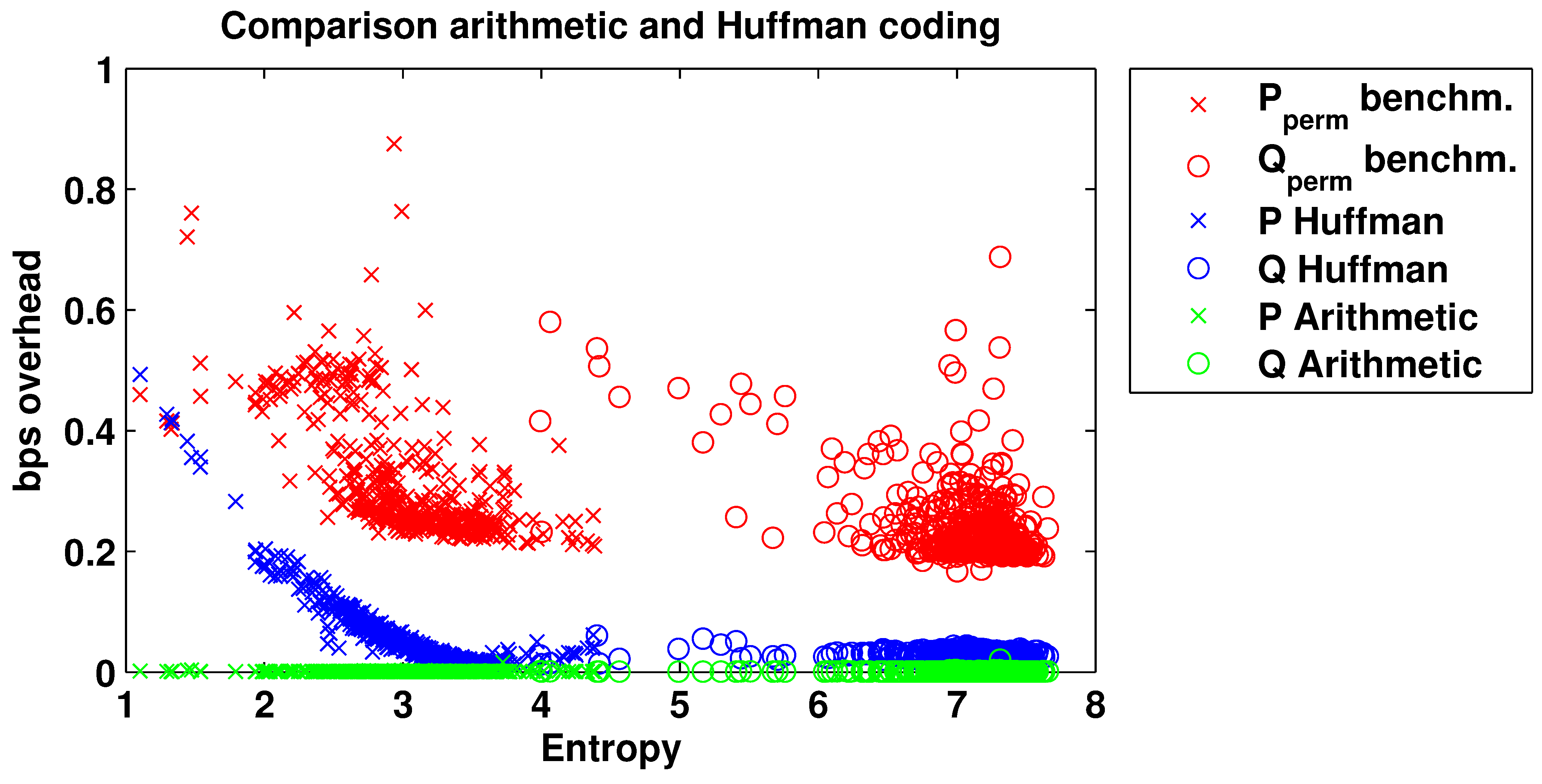
Figure 1. Overhead above the entropy limit of the best benchmark algorithm, Huffman coding, and arithmetic coding. The latter two exclude the dictionary.
Entropy 15 01289 g001

3.2. Reducing the Overhead

In order to explore the limits and overhead of distribution-based coding approaches, we tested the performance of Huffman coding and arithmetic coding when the distribution is known a priori. In other words, we looked at the resulting file size excluding the storage of the dictionary. As Figure 1 shows, the description length for the best benchmark compression of P is larger than the arithmetic code but incidentally smaller than the Huffman code. One basin had an overhead of 2.7 bits for P perm (not shown because out of scale). This is probably because that time series was relatively short compared with the others time series. The arithmetic code comes indistinguishably close to the entropy-bound. This indicates that a way forward for better compression is to find a description for the distribution that is shorter than the overhead of the existing algorithms over the arithmetic code. We will use both Huffman and arithmetic coding as back-ends for HydroZIP, which first tries to find improved probabilistic descriptions of the hydrological data that can be used to generate the dictionaries from a compact description.

3.3. The Structure in Hydrological Data

In this paper, we focus on time series of daily average Q and P, which are available for a large set of catchments. The types of structure found in these data, however, are also common at other time scales. An important part of the structure in rainfall–runoff data originates from the rainfall–runoff process. The fact that this structure exists makes streamflow prediction possible. It also allows efficient descriptions of rainfall and runoff time series when compressed together in one file. Such a file should then contain a form of a hydrological model, since that is hopefully an effective description of the rainfall–runoff process. We leave the exploration of rainfall–runoff models as compressors for future work, and in this paper we only consider single time series of either P or Q and focus on finding good time series models of them.
The structures we can exploit in the individual time series are the following:
  • Frequency distributions are generally smooth, allowing them to be parametrized instead of stored in a table.
  • Often longer dry periods occur, leading to series of zeros in rainfall and smooth recessions in streamflow.
  • Autocorrelation is often strong for streamflow, making entropy rate H ( X t | X t 1 ) significantly lower than the entropy H ( X t ) . Also, distribution of differences from one time step to the next will have a lower entropy: H ( X t X t 1 ) < H ( X t ) .
In this paper these forms of structure are used in HydroZIP to compactly describe hydrological data.
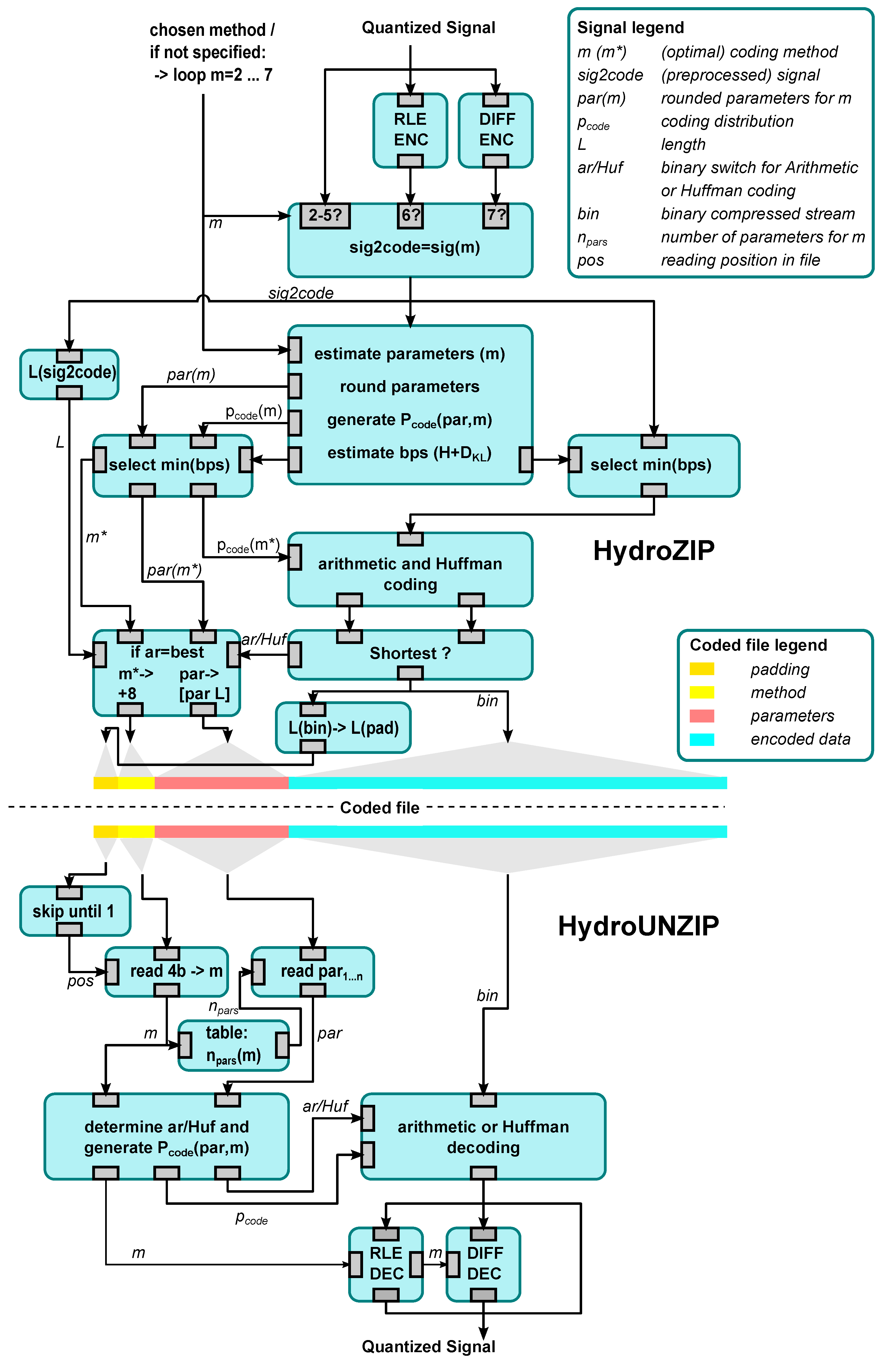
Figure 2. Flowchart of the HydroZIP and HydroUNZIP algorithms. For the coding, different parametric distributions are tried and their expected file sizes (bps) estimated using Equation (2). The most efficient parametric distribution description is then used to perform arithmetic coding and Huffman coding. The shortest bit stream of these two is then chosen and stored with the appropriate header information to decode. The decoding deciphers the header and then performs all reverse operations to yield the original signal.
Entropy 15 01289 g002

3.4. General Design of the Compressor and Compressed File

To achieve the shortest description of data, HydroZIP tries out compressing them by different approaches and afterward chooses the most effective (see Figure 2). For the description length, this flexibility in methods only comes at the cost of a few bits in the compressed file that specify which method was used to compress it, hence how to decompress it. Since for both Huffmann and arithmetic coding, the dictionary uniquely follows from the probabilities of the symbols to code, it is possible to decode the stream when the probabilities used to code the stream are known, which obviates the need to store the dictionary. Although probabilities that are equal to the frequencies result in an optimal dictionary, also approximate probabilities can be used for generating the dictionary and subsequent coding and decoding. When the approximation is good and can be described compactly, the compressor could outperform the ones that store the full dictionary in the compressed file.

3.5. Encoding the Distribution

The first step of the compressor is to try different parametric distributions as approximations for the marginal frequency distribution of the data. The file size can be estimated by
L = N D K L ( f | | g ) + H ( f ) + 8 M
in which L is the total number of bits to describe the data, N is the number of data points, D K L ( f | | g ) is the Kullback–Leibler divergence from frequency distribution vector f and approximated distribution vector g ( p code in Figure 2). M is the number of parameters needed to describe the distribution, which are coded with 8 bits each. L could also be written as
L = i = 1 N log ( g j i ) + 8 M
where g j i is the estimated probability assigned to the observed value j i at position i in the time series. Note the similarity with a maximum likelihood approach that includes a penalization for the number of parameters, such as the Akaike Information Criterion (AIC); [60,61].
The parametric distribution approximations that are tested are the Gaussian, exponential, P ( 0 ) + exponential for nonzero, P ( 0 ) + two parameter gamma for nonzero; see Figure 3 for examples. Furthermore, the skew-Laplace distribution is tested for the lag-1 differences of the data. Taking the differences is one of the pre-processing approaches described in the next subsection.
For all distributions, the parameters are first estimated from the data, and then mapped to a 0 to 255 range integer, which can be stored in one byte. The distribution is then regenerated from this rounded value and used for coding with one of the back-end coding mechanisms. This ensures that the distribution used for coding is exactly equal to the one that can be regenerated from the parameters stored in the compressed file.
Figure 3. Some examples of coding the data frequency distributions (in blue), approximating them (in red) with normal (left) and a two-parameter gamma distribution (right), where the probability of zeros occurring is coded as a separate parameter. The top row shows the data for Q, the bottom row for P, both from the basin of gauge nr. 1,321,000. Choosing the algorithm that leads to the smallest description length in bits per symbol (bps) is analogous to the inference of the most reasonable distribution: Gaussian for log(Q) and for P a probability of no rain plus a two parameter gamma for the rainy days. The entropy (H) and vector of 8 bit parameters are also shown.
Entropy 15 01289 g003

3.6. Efficient Description of Temporal Dependencies
To exploit the temporal dependencies in hydrological time series, two approaches were tried. Firstly, run length encoding (RLE [62]) of zeros is tried, which can make use of runs of zeros for rainfall series in dry climates or discharge in ephemeral streams. If three or more subsequent zeros are encountered, a special marker symbol ζ R L E is inserted (the number 256), followed by the number of zeros minus three. If a run of more than 258 zeros is encountered, it is stored as multiple separate runs to avoid confusion of the count with the marker symbol. The resulting RLE series, now consisting of 257 unique symbols, is coded using one of the parametric distributions mentioned in the previous subsection and subsequent arithmetic or Huffman coding.
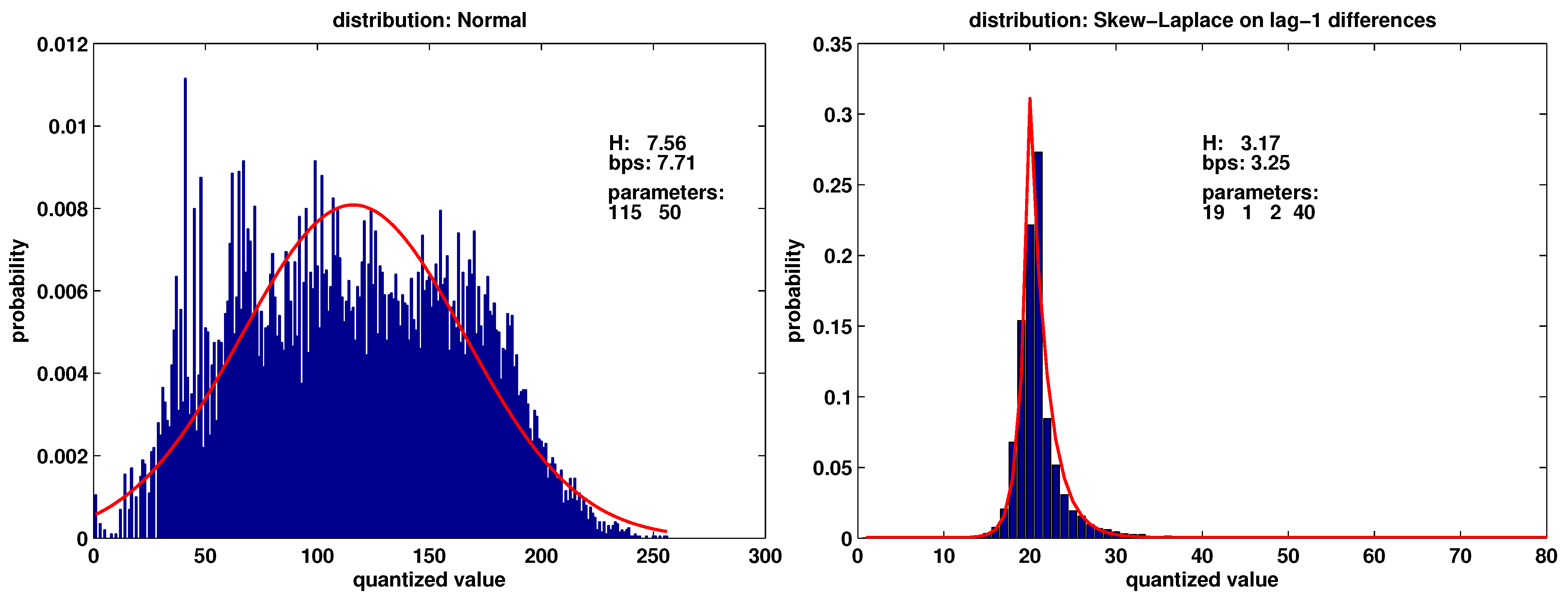
The second method takes the differences of each value with its preceding value. To avoid negative numbers in the transformed time series, the negative minimum δ is subtracted from the entire series and supplied as the first value of the series for decoding purposes. The frequency distribution of the resulting series of differences is approximated using skew-Laplace distribution, see Equation (4) and Figure 4 in the results section.
f ( x ; μ , α , β ) = α β α + β exp α μ x for x μ α β α + β exp β μ x for x > μ
Figure 4. Example of distributions of (left) streamflow coded with a normal distribution, and (right) of its lag-1 differences, coded as a skew-Laplace distribution. The entropy of the empirical distribution on the right is less than half of the original entropy, and can be quite well approximated with the skew-Laplace distribution (3.25 − 3.17 = 0.08 bps overhead).
Entropy 15 01289 g004

3.7. The Coded File

The coded file should be uniquely decodable and contain all information necessary to regenerate the original time series. The auxiliary information to decode the coded stream is stored in the header; see Figure 5. First, the padding serves to obtain a total file with an integer number of bytes, and consist of 1 to 8 bits that end after the first 1 is found. The following four bits tell the decompressor which of the 16 predefined methods was used to describe the distribution (currently, 12 are used, see Table 1). The number of parameters used by each method is predefined in the decompressor algorithm. Each parameter is stored in one byte, but if higher precision or a wider range is required, the methods could use e.g., two parameters to code and decode one high precision parameter.

3.8. HydroUNZIP

To check whether the information in the file is really an unambiguous, complete description of the data, a decoding algorithm, HydroUNZIP, was also developed. The HydroUNZIP algorithm (bottom part of Figure 2) first reads the header of the coded file to determine which of the predefined methods was used for compression and how many parameters have to be read. Subsequently, the appropriate distribution is reproduced and used for decoding the data part; depending on the method, this is done either with Huffman decoding or arithmetic decoding. Depending on the method specified in the header, these decoded data are then further decoded if necessary, using run length decoding or decoding the differences. The final output of HydroUNZIP should be exactly equal to the original time series that was coded using HydroZIP.
Figure 5. Schematic picture of the structure of the compressed file (colors correspond to Figure 2). The header describes the distribution, parameters and coding method of the data sequence. The padding ensures that the file can be written as an integer number of bytes.
Entropy 15 01289 g005
Table 1. The definition of the 12 current methods and corresponding parameters and ranges, which are mapped to an 8-bits unsigned integer. The method number is coded with 4 bits.
Parametric distributionnr.(Huf)nr.(ar)precodingparameters [range]
N ( μ , σ ) 210 μ , σ [0-255]
exp ( μ ) 311 μ[0-255]
exp ( μ x 0 ) + P ( 0 ) 412 μ x 0 [0-255]; P ( 0 ) [0-1]
Γ α , β + P ( 0 ) 513 α x 0 [0-5.1]; β x 0 [0-51]; P ( 0 ) [0-1]
Γ α , β + P ( 0 ) + P ( ζ R L E ) 614RLE α x 0 [0-5.1]; β x 0 [0-51]; P ( 0 ) , P ( ζ R L E ) [0-1]
skew-Laplace ( μ , α , β ) + K715Diff m u , α β [0-255], K[0-512]
The coded files were indeed confirmed to be lossless descriptions of the original data, reproducing them without errors. This means we can interpret the sizes of the compressed files as measures of information content, and the compressed files themselves as efficient descriptions or models of the data. The file sizes will be presented in the results.

4. Results

Resulting file sizes of the different compression algorithms can be interpreted as estimations of the information content of the data that were compressed. The description methods used to achieve efficient compression can be interpreted as models for those data. The comparison of HydroZIP results with the benchmark can serve to test whether hydrological knowledge leads to better models for hydrological data, when model adequacy is measured by compression efficiency. Furthermore the spatial patterns of compression results and most efficient methods are presented.

4.1. Results of the Benchmark Algorithms

Figure 6 gives an overview of the best compression rates achieved by existing algorithms on P and Q , as a function of location of the data. The results generally show a better compression for P, due to its lower entropy, but Q can often be compressed well below its entropy, due to the strong autocorrelation. Furthermore, it is visible that western climate, with more long dry spells, generally yields more compressible time series of P and Q. Note, however, that results should be interpreted with caution due to the influence of the scaling and quantization procedure used before compressing. For more elaborate discussion on the results of benchmark algorithms and spatial patterns, and a discussion on subjectivity of information content, see [5].
Figure 6. Spatial distribution of the compression results with the best benchmark algorithms for each time series of rainfall (left) and streamflow (right).
Entropy 15 01289 g006

4.2. Results for Compression with HydroZIP
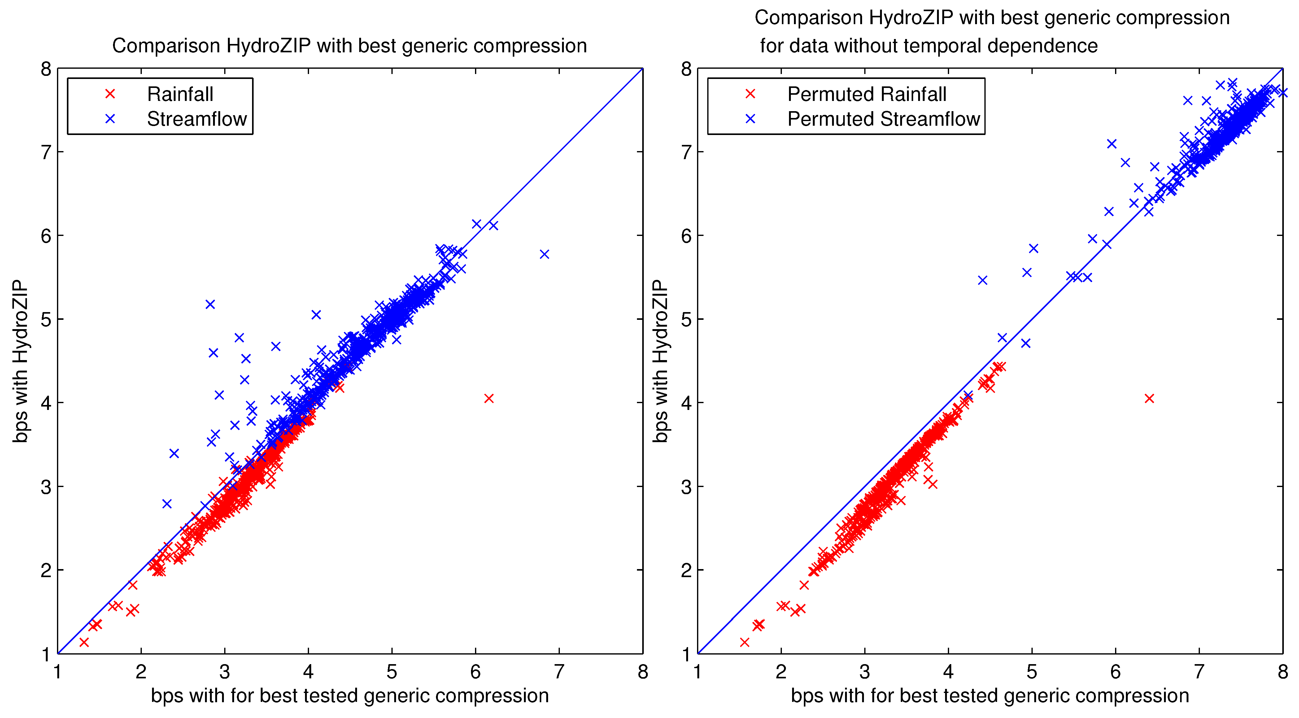
We can see from Figure 7 that HydroZIP outperformed the benchmark algorithms on all rainfall series and a good part of the streamflow series, with 90% of the compressed file size reductions falling between 1.4% and 11.8% for compression of P; see Table 2 for more statistics. For the permuted series on the right, where temporal dependencies cannot be exploited for compression, the results are even more pronounced. This result indicates that the main gain of HydroZIP is due to the efficient characterization of the distribution, and the fact that these parametric distributions are good fits to the hydrological data. The less pronounced difference in the original time series may indicate that there is still room for improvement for the coding of temporal dependencies, which apparently works well for some of the benchmark algorithms.
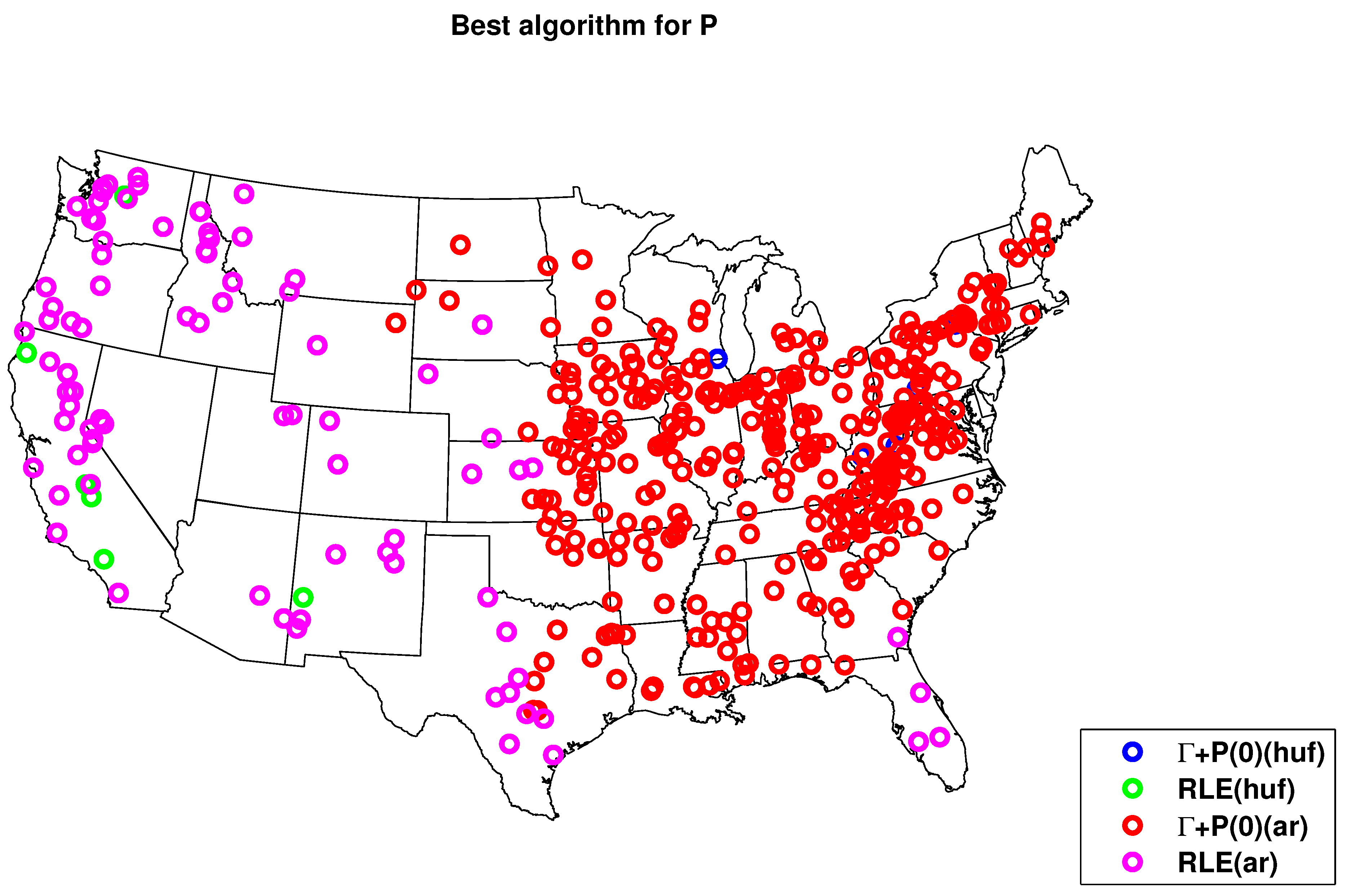
As can be seen from Figure 8, HydroZIP can outperform all benchmark algorithms in all basins by using an efficient description of a two parameter gamma distribution for wet days, and the probability of dry days as a separate parameter, either after run length encoding of the dry spells (legend: RLE) or directly (legend: Γ + P ( 0 ) ). Analogously, we can say that the compression experiment yielded the inference that daily precipitation is best modeled as a mixture of an occurrence process and a intensity process. This model is in line with [63,64], who also used AIC for model selection, which can be interpreted as analogous to our present approach of finding the shortest description for the data. Also the fact that we found the gamma distribution to be a powerful description for compression of the data is in line with the widespread use of the gamma distribution to describe daily rainfall amounts [65,66,67], although other distributions are sometimes found to behave better, especially in the tail [68]. In general, finding good compressors for environmental time series is completely analogous to modeling those series, such as done in, e.g., [69,70,71].
Figure 7. Comparison of file size after compression between HydroZIP and the best compression of the benchmark algorithms. Each point represents the data for one catchment. Points below the line indicate that HydroZIP outperforms the benchmark. The left figure shows results for the time series of rainfall and runoff. For the right figure, these time series are randomly permuted to exclude the effect of temporal dependencies.
Entropy 15 01289 g007
Table 2. Quantiles over the set of 431 basins of percentage file size reduction of HydroZIP over benchmark. Negative values indicate a larger file size for HydroZIP.
quantilefile size reduction (%)
PQPpermQperm
Min−2.5−83.23.515.0
5%1.4−9.64.748.4
50%5.5−0.36.857.7
95%11.82.817.070.5
Max34.215.436.783.5
Figure 8. Geographical spread of best performance compression methods for P.
Entropy 15 01289 g008
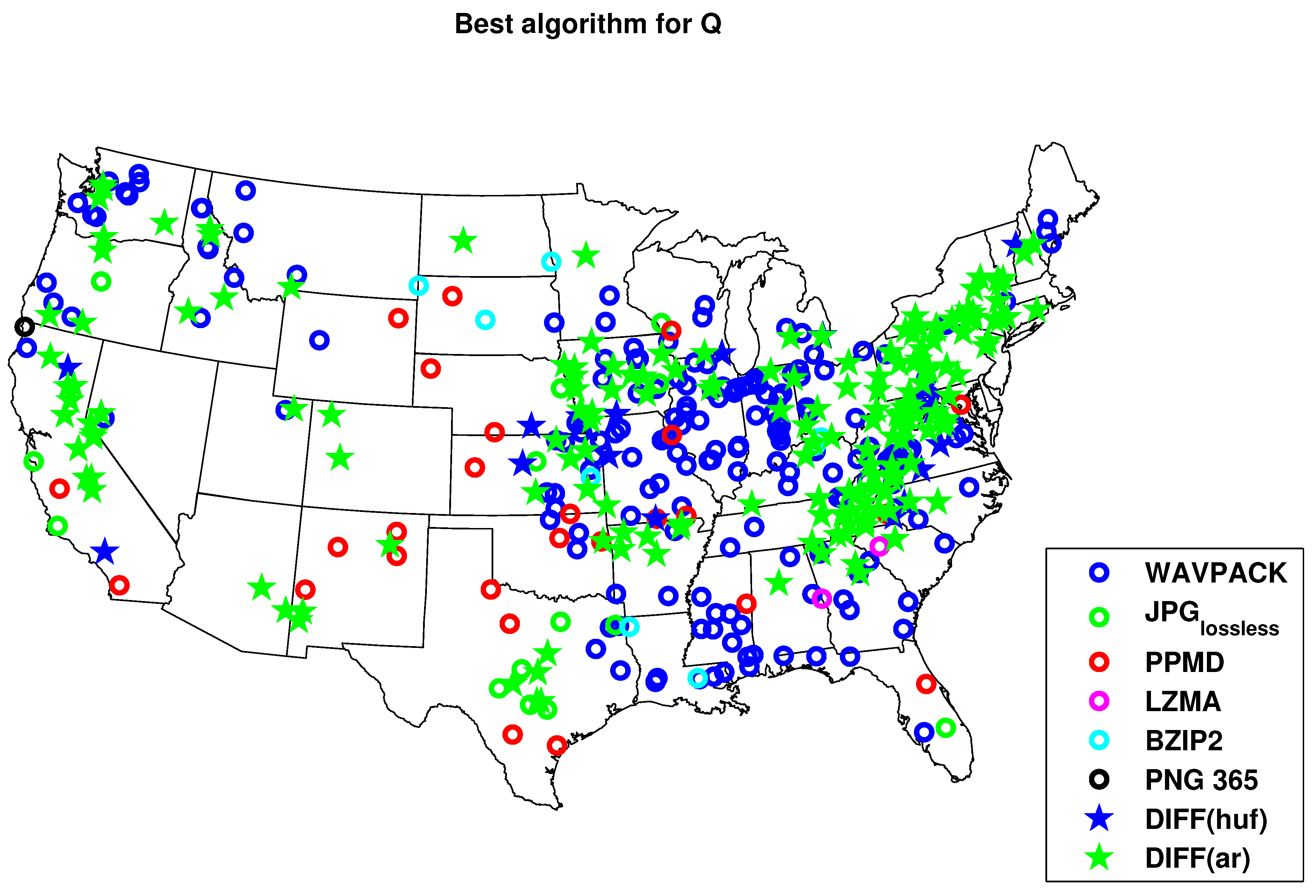
Figure 9. Geographical spread of best performance compression methods for Q. For the locations with circles, one of the benchmark algorithms performed best. The stars indicate the HydroZIP algorithm using coding of the differences.
Entropy 15 01289 g009
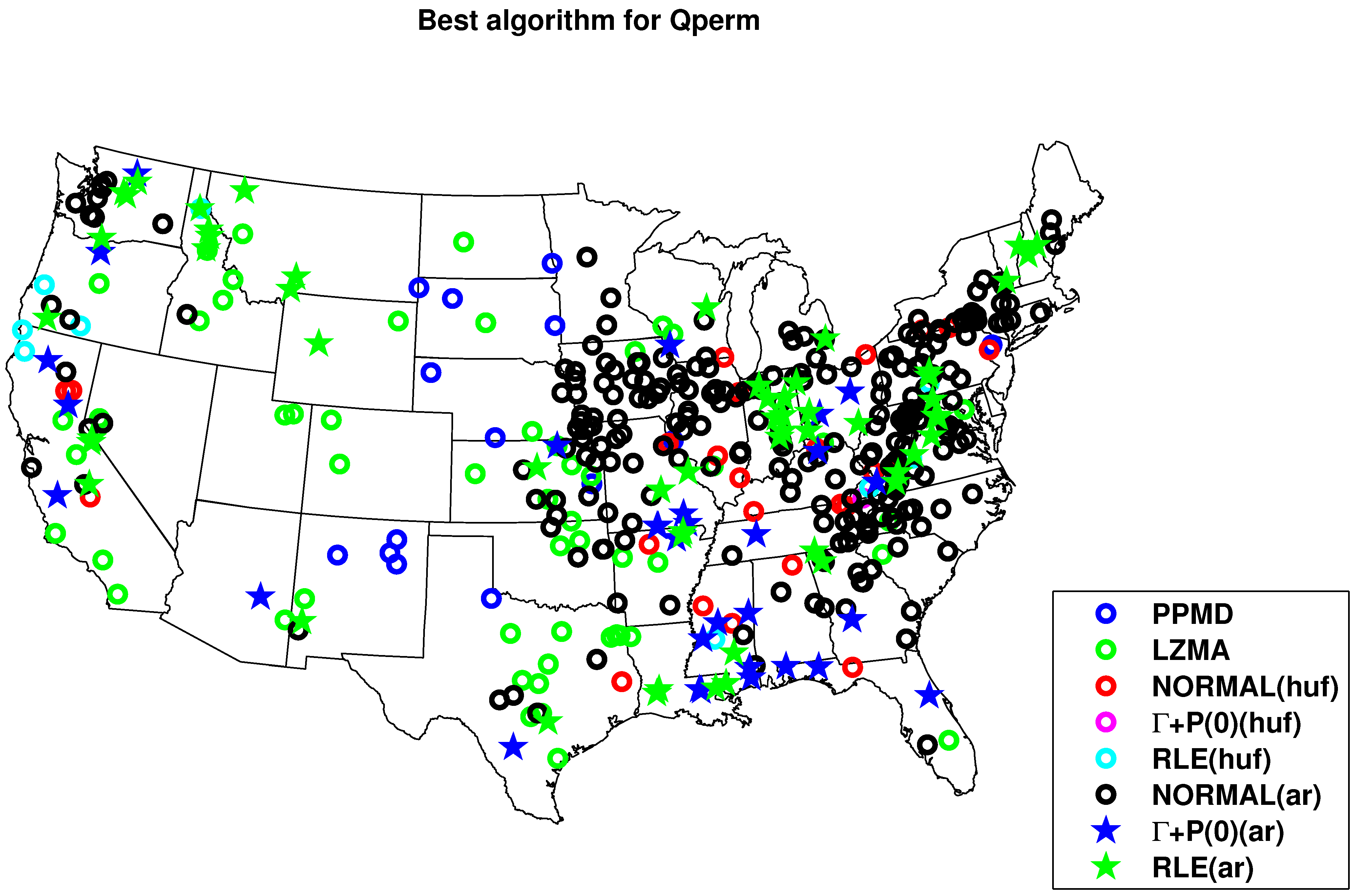
The best compression algorithms for streamflow show a more diverse geographical picture (Figure 9). Only in 199 out of 431 basins was HydroZIP able to outperform the best benchmark algorithm, using the method of coding the lag-1 differences with a skew-Laplace distribution (the stars in Figure 9); see Figure 4 for an example of the efficiency of this method. From Figure 10 it becomes clear that the better performance of the benchmark algorithms is mainly due to the efficient use of temporal dependencies in those algorithms, since for the randomly permuted series HydroZIP outperforms the benchmark in 364 out of 431 basins.
Figure 10. Geographical spread of best performance compression methods for the randomly permuted Q series. HydroZIP outperforms the benchmark everywhere except at the green and dark blue circles.
Entropy 15 01289 g010

5. Discussion and Conclusion

5.1. Discussion

Although the percentage gains in compression of HydroZIP over the benchmark are generally small and of limited use for practical compression use, they are significant from an inference-perspective. This significance stems from the fact the file sizes approach an unknown limit (the uncomputable Kolmogorov complexity of the data) from above. This means the percentage gain in terms of reduced redundancy above the limit is larger than the percentage file size decrease.
The results for compressing hydrological time series with our hydrology-specific compressor, HydroZIP, showed that indeed we were able to improve compression ratios of the best generic compression algorithms in our benchmark set. This improvement confirms the theoretical notion that prior knowledge about data structure should lead to better compression, or equivalently to better predictions of the data points. For rainfall, the prior knowledge allowed us to outperform all benchmark algorithms over all tested river basins. The prior knowledge that improved the compression for rainfall includes:
  • rainfall amounts can be described by a smooth, parametric distribution
  • dry days may be modeled separately
  • dry spells have the tendency to persist for multiple days, or even months
  • several candidate distributions from hydrological literature
In contrast, the prior knowledge in most benchmark compression algorithms does not assume any smoothness in the distributions; rather, they store a full dictionary optimized for the occurrence frequencies of the data. Furthermore the benchmark algorithms look for reoccurring sequences that are common in, e.g., text files, but in complex hydrological systems, nature rarely repeats its own behaviour exactly.
From a model complexity perspective, we can say that the full dictionary is a description that is too long compared with the amount of data coded with it or, analogously, that the 256 bin histogram is a model too complex for the data. If seen in a Bayesian framework, the dictionary is a model with a long description, hence a small prior probability [15,21]. Even though the coded data will be shorter because the codes correspond better to the frequency distribution of the data (analogous to a higher likelihood), this gain is offset by the description of the dictionary (the lower prior). In HydroZIP, the data are less efficiently coded, but the file header is very short compared with the full dictionary. This coding can be interpreted as a model with lower likelihood, but higher prior probability. The shorter total description indicates that the posterior probability of the parametric model is higher than that of the histogram, because model complexity and amount of data are balanced better. Furthermore, it is likely that if new data from the same source were compressed using the same codewords, the simpler model used in HydroZIP would yield a similar performance as on the old data, while the more complex model would perform worse, because the histogram will now be not optimally tuned to the frequencies, therefore losing the likelihood advantage but still keeping the prior disadvantage. Stated differently, over-fitted models perform worse in prediction.
In our consideration of description length, we did not include the size of the decompression algorithm executable file. This size should be included to apply the algorithmic information theory framework correctly. At the present stage, it is difficult to determine the algorithm size, since it consists of a set of MATLAB functions that also use existing toolboxes, but we hope to address this in future work. It should be noted that our decompression algorithm is universal for the whole MOPEX data set, and any time-series-specific information is stored in the compressed file and counted toward the description length. Consequently, the size of the decompression algorithms can be divided over the number of data points of the entire data set when considering this additional complexity penalization. It is therefore expected that this will not have a large influence on the results presented in bits per symbol.

5.2. Caveats and Future Work

In this work, we considered individual time series of P and Q and looked for ways to describe their internal dependencies efficiently by using hydrological knowledge. However, a more central problem in hydrology is the prediction of various components of the hydrological cycle, based on knowledge of other components and properties of the system. The most classical example is the prediction of streamflow from precipitation. These rainfall–runoff models should theoretically help to compress combined data sets of rainfall and streamflow. Conversely, finding the best compression algorithm should result in something that looks like a rainfall–runoff model, combined with an efficient description of internal dependencies of rainfall. This combined compression is the subject of an ongoing investigation where hydrological models are incorporated into the compression procedure. The compression framework also offers new ways to interpret a decomposition of Kullback–Leibler divergence in the context of forecast verification of probabilistic forecasts [37].
Another point that is worth further investigation is the pre-treatment and quantization of the data. In the present study, the starting points were pre-processed series that were scaled and quantized to a integers over an 8 bit range. These integers were subsequently coded with lossless compression algorithms. Nevertheless, a loss of information already occurs in the quantization step, hence it would be an interesting next step to consider the combined preprocessing, scaling, quantization and coding as one process of lossy compression. This will allow considering optimal quantization schemes and information loss versus description efficiency. This trade-off can be related to measurement accuracy and true information content of measured data, especially in the context of structural measurement errors [72,73].
Furthermore, the scaling could be considered as an integral part of the description process. It would be more natural not to assume the minimum and maximum values of the time series as known a priori. In reality, these values are important pieces of information that are learned from a time series. In our present study, this aspect is somewhat clouded by the scaling, which makes the data seem more regular and less surprising than is usually the case in nature. On the other hand, when a high peak occurs, the scaling will compress the rest of the series in a smaller range. This causes a reverse effect by making the data seem less informative. Hence, in the present study the mapping of the original information content in the time series to that of the quantized time series should be interpreted with caution. The subjectivity of this mapping is a general problem when determining information content of time series that becomes explicit when using information-theoretical methods.
In future research, we also plan to include more alternative distributions in HydroZIP so that it becomes a more complete inference framework and can achieve better compression.

5.3. Conclusion

As a first attempt of including hydrological knowledge in the compression of hydrological data, we were able to show that indeed compression rates could be enhanced in many cases. This opens up an interesting line of research in which inferences are used for better compression, but this compression is also used as a natural framework to view the way we learn from hydrological data. This puts information in a central role for model inference and prediction across scales, which are the core tasks but also the main challenges of hydrology.

Acknowledgments

Steven Weijs is a beneficiary of a postdoctoral fellowship from the AXA research fund, which is gratefully acknowledged. Funding from the Swiss Science Foundation, the NCCR-MICS and CCES are also gratefully acknowledged. We thank both anonymous reviewers for their constructive comments, which helped improve the presentation of this manuscript.

References

  1. Lehning, M.; Dawes, N.; Bavay, M.; Parlange, M.; Nath, S.; Zhao, F. Instrumenting the Earth: Next-generation Sensor Networks and Environmental Science. In The Fourth Paradigm: Data-Intensive Scientific Discovery; Microsoft Research: Redmond, WA, USA, 2009. [Google Scholar]
  2. Ryabko, B.; Astola, J. Application of Data Compression Methods to Hypothesis Testing for Ergodic and Stationary Processes. In Proceedings of the International Conference on Analysis of Algorithms DMTCS Proceedings AD, Barcelona, Spain, 6–10 June, 2005; Volume 399, p. 408.
  3. Ryabko, B.; Astola, J.; Gammerman, A. Application of Kolmogorov complexity and universal codes to identity testing and nonparametric testing of serial independence for time series. Theor. Comput. Sci. 2006, 359, 440–448. [Google Scholar] [CrossRef]
  4. Cilibrasi, R. Statistical inference through data compression. Ph.D. Thesis, Universiteit van Amsterdam, Amsterdam, The Netherlands, 2007. [Google Scholar]
  5. Weijs, S.V.; van de Giesen, N.; Parlange, M.B. Data compression to define information content of hydrological time series. Hydrol. Earth Syst. Sci. Discuss. 2013, 10, 2029–2065. [Google Scholar] [CrossRef]
  6. Kavetski, D.; Kuczera, G.; Franks, S.W. Bayesian analysis of input uncertainty in hydrological modeling: 1. Theory. Water Resour. Res. 2006, 42. [Google Scholar] [CrossRef]
  7. Beven, K.; Smith, P.; Wood, A. On the colour and spin of epistemic error (and what we might do about it). Hydrol. Earth Syst. Sci. 2011, 15, 3123–3133. [Google Scholar] [CrossRef]
  8. Singh, S.K.; Bárdossy, A. Calibration of hydrological models on hydrologically unusual events. Adv. Water Resour. 2012, 38, 81–91. [Google Scholar] [CrossRef]
  9. Gong, W.; Gupta, H.V.; Yang, D.; Sricharan, K.; Hero, A.O. Estimating epistemic & aleatory uncertainties during hydrologic modeling: An information theoretic approach. Water Resour. Res. 2013, in press. [Google Scholar]
  10. Stedinger, J.R.; Vogel, R.M.; Lee, S.U.; Batchelder, R. Appraisal of the generalized likelihood uncertainty estimation (GLUE) method. Water Resour. Res. 2008, 44. [Google Scholar] [CrossRef]
  11. Montanari, A.; Shoemaker, C.A.; van de Giesen, N. Introduction to special section on Uncertainty Assessment in Surface and Subsurface Hydrology: An overview of issues and challenges. Water Resour. Res. 2009, 45. [Google Scholar] [CrossRef]
  12. Montanari, A.; Koutsoyiannis, D. A blueprint for process-based modeling of uncertain hydrological systems. Water Resour. Res. 2012, 48. [Google Scholar] [CrossRef]
  13. Collins English Dictionary-Complete & Unabridged 10th Edition. Available online: http://www.collinsdictionary.com/dictionary/english/zip (accessed on 14 March 2013).
  14. Chaitin, G.J. On the length of programs for computing finite binary sequences. J. ACM 1966, 13, 547–569. [Google Scholar] [CrossRef]
  15. Solomonoff, R.J. A formal theory of inductive inference. Part I. Inform. Control 1964, 7, 1–22. [Google Scholar] [CrossRef]
  16. Kolmogorov, A.N. Three approaches to the quantitative definition of information. Int. J. Comput. Math. 1968, 2, 157–168. [Google Scholar] [CrossRef]
  17. Chaitin, G.J. A theory of program size formally identical to information theory. J. ACM 1975, 22, 329–340. [Google Scholar] [CrossRef]
  18. Rissanen, J. Information and Complexity in Statistical Modeling; Springer Verlag: New York, NY, USA, 2007. [Google Scholar]
  19. Schoups, G.; van de Giesen, N.C.; Savenije, H.H.G. Model complexity control for hydrologic prediction. Water Resour. Res. 2008, 44. [Google Scholar] [CrossRef]
  20. Jaynes, E.T. Probability Theory: The Logic of Science; Cambridge University Press: Cambridge, UK, 2003. [Google Scholar]
  21. Hutter, M. On universal prediction and Bayesian confirmation. Theor. Comput. Sci. 2007, 384, 33–48. [Google Scholar] [CrossRef]
  22. Rathmanner, S.; Hutter, M. A philosophical treatise of universal induction. Entropy 2011, 13, 1076–1136. [Google Scholar] [CrossRef]
  23. Cilibrasi, R.; Vitányi, P. Clustering by compression. IEEE Trans. Inform. Theory 2005, 51, 1523–1545. [Google Scholar] [CrossRef]
  24. Vitányi, P.; Balbach, F.; Cilibrasi, R.; Li, M. Normalized Information Distance. In Information Theory and Statistical Learning; Emmert-Streib, F., Dehmer, M., Eds.; Springer: New York, NY, USA, 2009; pp. 45–82. [Google Scholar]
  25. Cerra, D.; Datcu, M. Expanding the algorithmic information theory frame for applications to earth observation. Entropy 2013, 15, 407–415. [Google Scholar] [CrossRef]
  26. Szilagyi, J.; Parlange, M. A geomorphology-based semi-distributed watershed model. Adv. Water Resour. 1999, 23, 177–187. [Google Scholar] [CrossRef]
  27. Beven, K.J. How far can we go in distributed hydrological modelling? Hydrol. Earth Syst. Sci. 2001, 5, 1–12. [Google Scholar] [CrossRef]
  28. Simoni, S.; Padoan, S.; Nadeau, D.; Diebold, M.; Porporato, A.; Barrenetxea, G.; Ingelrest, F.; Vetterli, M.; Parlange, M. Hydrologic response of an alpine watershed: Application of a meteorological wireless sensor network to understand streamflow generation. Water Resour. Res. 2011, 47. [Google Scholar] [CrossRef]
  29. Leung, L.Y.; North, G.R. Information theory and climate prediction. J. Clim. 1990, 3, 5–14. [Google Scholar] [CrossRef]
  30. Kleeman, R. Measuring dynamical prediction utility using relative entropy. J. Atmos. Sci. 2002, 59, 2057–2072. [Google Scholar] [CrossRef]
  31. DelSole, T. Predictability and information theory. Part I: Measures of predictability. J. Atmos. Sci. 2004, 61, 2425–2440. [Google Scholar] [CrossRef]
  32. DelSole, T.; Tippett, M.K. Predictability: Recent insights from information theory. Rev. Geophys. 2007, 45. [Google Scholar] [CrossRef]
  33. Roulston, M.S.; Smith, L.A. Evaluating probabilistic forecasts using information theory. Mon. Weather Rev. 2002, 130, 1653–1660. [Google Scholar] [CrossRef]
  34. Benedetti, R. Scoring rules for forecast verification. Mon. Weather Rev. 2010, 138, 203–211. [Google Scholar]
  35. Ahrens, B.; Walser, A. Information-based skill scores for probabilistic forecasts. Mon. Weather Rev. 2008, 136, 352–363. [Google Scholar] [CrossRef]
  36. Tödter, J.; Ahrens, B. Generalization of the ignorance score: Continuous ranked version and its decomposition. Mon. Weather Rev. 2012, 140, 2005–2017. [Google Scholar]
  37. Weijs, S.V.; van Nooijen, R.; van de Giesen, N. Kullback–Leibler divergence as a forecast skill score with classic reliability–resolution–uncertainty decomposition. Mon. Weather Rev. 2010, 138, 3387–3399. [Google Scholar] [CrossRef]
  38. Weijs, S.V.; Schoups, G.; van de Giesen, N. Why hydrological predictions should be evaluated using information theory. Hydrol. Earth Syst. Sci. 2010, 14, 2545–2558. [Google Scholar] [CrossRef]
  39. Harmancioglu, N.B.; Alpaslan, N.; Singh, V.P. Application of the Entropy Concept in Design of Water Quality Monitoring Networks. In Entropy and Energy Dissipation in Water Resources; Singh, V., Fiorentino, M., Eds.; Kluwer Academic Publishers: Dordrecht, The Netherlands, 1992; pp. 283–302. [Google Scholar]
  40. Alfonso, L.; Lobbrecht, A.; Price, R. Information theory-based approach for location of monitoring water level gauges in polders. Water Resour. Res. 2010, 46. [Google Scholar] [CrossRef]
  41. Li, C.; Singh, V.; Mishra, A. Entropy theory-based criterion for hydrometric network evaluation and design: Maximum information minimum redundancy. Water Resour. Res. 2012, 48. [Google Scholar] [CrossRef]
  42. Singh, V.P. The use of entropy in hydrology and water resources. Hydrol. Process. 1997, 11, 587–626. [Google Scholar] [CrossRef]
  43. Lange, H. Are ecosystems dynamical systems. Int. J. Comput. Anticip. Syst. 1998, 3, 169–186. [Google Scholar]
  44. Lange, H. Time series analysis of ecosystem variables with complexity measures. Int. J. Complex Syst. 1999, 250, 1–9. [Google Scholar]
  45. Gupta, H.V.; Sorooshian, S.; Yapo, P.O. Toward improved calibration of hydrologic models: Multiple and noncommensurable measures of information. Water Resour. Res. 1998, 34, 751–763. [Google Scholar] [CrossRef]
  46. Vrugt, J.; Bouten, W.; Weerts, A. Information content of data for identifying soil hydraulic parameters from outflow experiments. Soil Sci. Soc. Am. J. 2001, 65, 19–27. [Google Scholar] [CrossRef]
  47. Vrugt, J.A.; Bouten, W.; Gupta, H.V.; Sorooshian, S. Toward improved identifiability of hydrologic model parameters: The information content of experimental data. Water Resour. Res. 2002, 38. [Google Scholar] [CrossRef]
  48. Laio, F.; Allamano, P.; Claps, P. Exploiting the information content of hydrological “outliers” for goodness-of-fit testing. Hydrol. Earth Syst. Sci. 2010, 14, 1909–1917. [Google Scholar] [CrossRef]
  49. Price, J. Comparison of the information content of data from the Landsat-4 Thematic Mapper and the Multispectral Scanner. Geosci. Remote Sens. IEEE Trans. 1984, 3, 272–281. [Google Scholar] [CrossRef]
  50. Horvath, K.; Stogner, H.; Weinhandel, G.; Uhl, A. Experimental Study on Lossless Compression of Biometric Iris Data. In Proceedings of the 7th International Symposium on Image and Signal Processing and Analysis (ISPA), Dubrovnik, Croatia, 4–6 September 2011; pp. 379–384.
  51. Nalbantoglu, O.U.; Russell, D.J.; Sayood, K. Data compression concepts and algorithms and their applications to bioinformatics. Entropy 2009, 12, 34–52. [Google Scholar] [CrossRef] [PubMed]
  52. Voepel, H.; Ruddell, B.; Schumer, R.; Troch, P.; Brooks, P.; Neal, A.; Durcik, M.; Sivapalan, M. Quantifying the role of climate and landscape characteristics on hydrologic partitioning and vegetation response. Water Resour. Res. 2011, 47. [Google Scholar] [CrossRef]
  53. Weijs, S.V.; Mutzner, R.; Parlange, M.B. Could electrical conductivity replace water level in rating curves for alpine streams? Water Resour. Res. 2013, 49, 343–351. [Google Scholar] [CrossRef]
  54. Huffman, D.A. A method for the construction of minimum-redundancy codes. Proc. IRE 1952, 40, 1098–1101. [Google Scholar] [CrossRef]
  55. Ziv, J.; Lempel, A. A universal algorithm for sequential data compression. IEEE Trans. Inform. Theory 1977, 23, 337–343. [Google Scholar] [CrossRef]
  56. Martin, G.N.N. Range Encoding: An Algorithm for Removing Redundancy from a Digitised Message. In Proceedings of the Video & Data Recording Conference, Southampton, UK, 24–27 July 1979.
  57. Rissanen, J.; Langdon, G.G. Arithmetic coding. IBM J. Res. Dev. 1979, 23, 149–162. [Google Scholar] [CrossRef]
  58. Burrows, M.; Wheeler, D.J. A Block-sorting Lossless Data Compression Algorithm, Technical report; Systems Research Center: Palo Alto, CA, USA, 1994. [Google Scholar]
  59. Shannon, C.E. A mathematical theory of communication. Bell Syst. Tech. J. 1948, 27, 379–423. [Google Scholar] [CrossRef]
  60. Akaike, H. Information Theory and an Extension of the Maximum Likelihood Principle. In Proceedings of the 2nd International Symposium on Information Theory, Tsahkadsor, Armenia SSR, 2–8 September 1973; pp. 267–281.
  61. Akaike, H. A new look at the statistical model identification. IEEE Trans. Autom. Control 1974, 19, 716–723. [Google Scholar] [CrossRef]
  62. Michel, W.S. Statistical encoding for text and picture communication. Am. Inst. Electr. Eng. Part I Commun. Electron. Trans. 1958, 77, 33–36. [Google Scholar] [CrossRef]
  63. Katz, R.; Parlange, M. Effects of an index of atmospheric circulation on stochastic properties of precipitation. Water Resour. Res. 1993, 29, 2335–2344. [Google Scholar] [CrossRef]
  64. Parlange, M.B.; Katz, R.W. An extended version of the Richardson model for simulating daily weather variables. J. Appl. Meteorol. 2000, 39, 610–622. [Google Scholar] [CrossRef]
  65. Katz, R.W. Extreme value theory for precipitation: Sensitivity analysis for climate change. Adv. Water Resour. 1999, 23, 133–139. [Google Scholar] [CrossRef]
  66. Groisman, P.Y.; Karl, T.R.; Easterling, D.R.; Knight, R.W.; Jamason, P.F.; Hennessy, K.J.; Suppiah, R.; Page, C.M.; Wibig, J.; Fortuniak, K.; et al. Changes in the probability of heavy precipitation: Important indicators of climatic change. Clim. Chang. 1999, 42, 243–283. [Google Scholar] [CrossRef]
  67. Semenov, V.; Bengtsson, L. Secular trends in daily precipitation characteristics: Greenhouse gas simulation with a coupled AOGCM. Clim. Dyn. 2002, 19, 123–140. [Google Scholar]
  68. Papalexiou, S.; Koutsoyiannis, D. Entropy based derivation of probability distributions: A case study to daily rainfall. Adv. Water Resour. 2011, 45, 51–57. [Google Scholar] [CrossRef]
  69. Szilagyi, J.; Katul, G.G.; Parlange, M.B. Evapotranspiration intensifies over the conterminous United States. J. Water Resour. Plan. Manag. 2001, 127, 354–362. [Google Scholar] [CrossRef]
  70. Katz, R.W.; Parlange, M.B.; Tebaldi, C. Stochastic modeling of the effects of large-scale circulation on daily weather in the southeastern US. Clim. Chang. 2003, 60, 189–216. [Google Scholar] [CrossRef]
  71. Katz, R.W.; Brush, G.S.; Parlange, M.B. Statistics of extremes: Modeling ecological disturbances. Ecology 2005, 86, 1124–1134. [Google Scholar] [CrossRef]
  72. Beven, K.; Westerberg, I. On red herrings and real herrings: Disinformation and information in hydrological inference. Hydrol. Process. 2011, 25, 1676–1680. [Google Scholar] [CrossRef]
  73. Weijs, S.V.; van de Giesen, N. Accounting for observational uncertainty in forecast verification: An information–theoretical view on forecasts, observations and truth. Mon. Weather Rev. 2011, 139, 2156–2162. [Google Scholar] [CrossRef]