Generalized Statistical Mechanics at the Onset of Chaos

Abstract

Transitions to chaos in archetypal low-dimensional nonlinear maps offer real and precise model systems in which to assess proposed generalizations of statistical mechanics. The known association of chaotic dynamics with the structure of Boltzmann–Gibbs (BG) statistical mechanics has suggested the potential verification of these generalizations at the onset of chaos, when the only Lyapunov exponent vanishes and ergodic and mixing properties cease to hold. There are three well-known routes to chaos in these deterministic dissipative systems, period-doubling, quasi-periodicity and intermittency, which provide the setting in which to explore the limit of validity of the standard BG structure. It has been shown that there is a rich and intricate behavior for both the dynamics within and towards the attractors at the onset of chaos and that these two kinds of properties are linked via generalized statistical-mechanical expressions. Amongst the topics presented are: (i) permanently growing sensitivity fluctuations and their infinite family of generalized Pesin identities; (ii) the emergence of statistical-mechanical structures in the dynamics along the routes to chaos; (iii) dynamical hierarchies with modular organization; and (iv) limit distributions of sums of deterministic variables. The occurrence of generalized entropy properties in condensed-matter physical systems is illustrated by considering critical fluctuations, localization transition and glass formation. We complete our presentation with the description of the manifestations of the dynamics at the transitions to chaos in various kinds of complex systems, such as, frequency and size rank distributions and complex network images of time series. We discuss the results.

1. Introduction

Chaotic dynamical systems, such as chaotic attractors in one-dimensional nonlinear iterated maps, accept a statistical-mechanical description with an entropy expression of the Boltzmann–Gibbs (BG) type [1]. The chaotic attractors generated by these maps have ergodic and mixing properties, and not surprisingly, they can be described by a thermodynamic formalism compatible with BG statistics [1]. However, at the transition to chaos, such as the period-doubling accumulation point, the so-called Feigenbaum attractor, these two properties are lost, and this suggests the possibility of exploring the limit of validity of the BG structure in a precise, but simple enough, setting.

The attractors at the transitions to chaos in one-dimensional nonlinear maps (that we shall refer to as critical attractors) have a vanishing ordinary Lyapunov coefficient, ${\lambda }_1$, and the sensitivity to initial conditions, ${\xi }_t$, for large iteration time t ceases to obey exponential behavior, exhibiting, instead, power-law or faster than exponential growth behavior [2,3,4,5,6,7]. As it is generally suggested, the standard exponential divergence of trajectories in chaotic attractors provides a mechanism to justify the assumption of irreversibility in the BG statistical mechanics [1]. In contrast, the onset of chaos in (necessarily dissipative) one-dimensional maps imprints memory preserving phase-space properties to its trajectories [2], and we consider them here with a view to assess if generalized entropy expressions replace the usual BG expression. A simple type of attractor with ${\lambda }_1=0$ occurs at the transitions between periodic orbits, the so-called pitchfork bifurcations along the period-doubling cascades [8,9]. Another type, a critical attractor-repellor pair, occurs at the tangent bifurcation [8,9], a central feature for the intermittency route to chaos. Perhaps the most interesting types of critical attractors are geometrically involved (multifractal) sets of positions for which trajectories within them display an ever fluctuating non-exponential sensitivity, ${\xi }_t$ [2]. Important examples are the onset of chaos via period doubling and via quasiperiodicity, two other universal routes to chaos exhibited, respectively, by the prototypical logistic and circle maps [8,9].

There are two sets of properties associated with the attractors involved: those of the dynamics inside the attractors and those of the dynamics towards the attractors. These properties have been characterized in detail for the Feigenbaum attractor; both the organization of trajectories and the sensitivity to initial conditions are described in [4], while the features of the rate of approach of an ensemble of trajectories to this attractor appears, explained in [5]. The dynamics inside quasiperiodic critical attractors has also been determined by considering the so-called golden route to chaos in the circle map [6]. The patterns formed by trajectories and the sensitivity, ${\xi }_t$, in this different case were found to share the general scheme displayed by these quantities for the Feigenbaum point, but with somewhat more involved features [6]. On the contrary, the critical attractor-repellor set at the tangent bifurcation is a simpler finite set of positions with periodic dynamics that can be reduced to a single period-one attractor-repellor fixed point via functional composition, and the interesting properties of trajectories and sensitivity, ${\xi }_t$, correspond to the dynamics towards the attractor or away from the repellor [3]. The search for generalized entropy properties in the dynamics of critical attractors has been two-fold. One focal point has been the determination of Pesin-like identities associated with the sensitivity, ${\xi }_t$, within multifractal critical attractors for which the entropy expression involved is different from the BG expression. The second focal point is the determination of the relationship between the dynamics towards and the dynamics within multifractal critical attractors for which it has been found that the expression linking the two types of dynamics is statistical-mechanical in nature, one in which the configurational weights and the thermodynamical potential expressions differ from the BG ordinary exponential and logarithmic expressions. The simpler case of the tangent bifurcation also involves generalized entropy expressions linked to the trajectories and the sensitivity of the dynamics towards or away from the attractor-repellor fixed point.

The generalized entropy expressions were found to be of the Tsallis or q -statistical type [10,11], involving the “q-deformed” logarithmic function ${ln}_{q}y\equiv (y^{1-q}-1)/(1-q)$, the functional inverse of the “q-deformed” exponential function ${exp}_q(x)\equiv {[1-(q-1)x]}^{-1/(q-1)}$. For the pitchfork and tangent bifurcations, the trajectories and the sensitivity, ${\xi }_t$ (of their functional-composition renormalization-group (RG) fixed-point maps), are exactly expressible by q-exponentials, and this leads to generalized q-Lyapunov exponents ${\lambda }_q$ that are dependent on initial conditions [3]. For multifractal critical attractors, the sensitivity, ${\xi }_t$, was found to be expressible in terms of an infinite set of q-exponential functions, and from such ${\xi }_t$, one or several spectra of q-generalized Lyapunov coefficients ${\lambda }_q$ were determined. The ${\lambda }_q$ are dependent on the initial position, $x_0$, and each spectrum can be examined by varying this position. The ${\lambda }_q$ satisfy a q-generalized identity ${\lambda }_q=K_q$ of the Pesin type [9], where $K_q$ is an entropy production rate based on q-statistical-type entropy expressions $S_q$ [4,6]. In all cases, the presence of dual q-indexes, q and $2-q$, or q and $1/q$, or a combination of them, have all well-defined dynamical meanings. If there is an entropy, $S_q$, or a coefficient, ${\lambda }_q$, in the description of a critical attractor, the quantities, $S_{2-q}$ and ${\lambda }_{2-q}$, complement that description [4,6] . The partition function that describes the approach of trajectories to the Feigenbaum attractor contains an infinite set of q-exponential weights (stemming from the infinite set of universal constants associated with the attractor), and the resulting thermodynamic potential involves another q-index, which is the complicated outcome of all q-indexes involved in the configurational terms [5]. The generalized entropy in this case differs from the scheme contained in [10,11].

The manifestation of q-statistics in complex condensed-matter systems can be explored via connections that have been established between the dynamics of critical attractors and the dynamics taking place in, for example, thermal systems under conditions when mixing and ergodic properties are not easily fulfilled. A relationship between intermittency and critical fluctuations suggested [12,13] that the dynamics in the proximity of a tangent bifurcation is analogous to the dynamics of fluctuations of an equilibrium state with well-known scaling properties [14,15]. 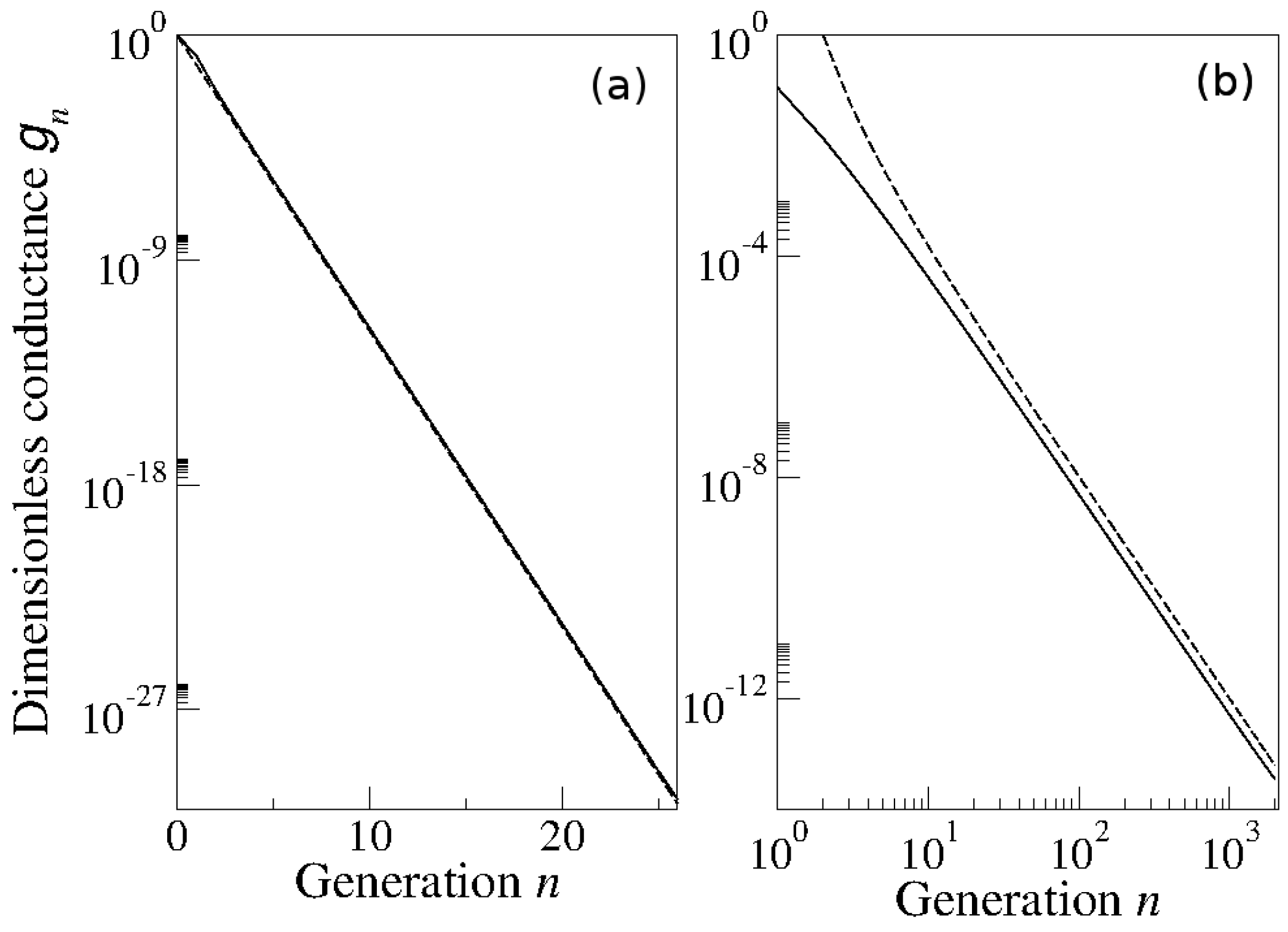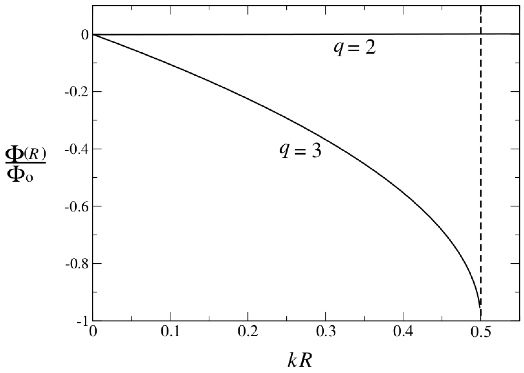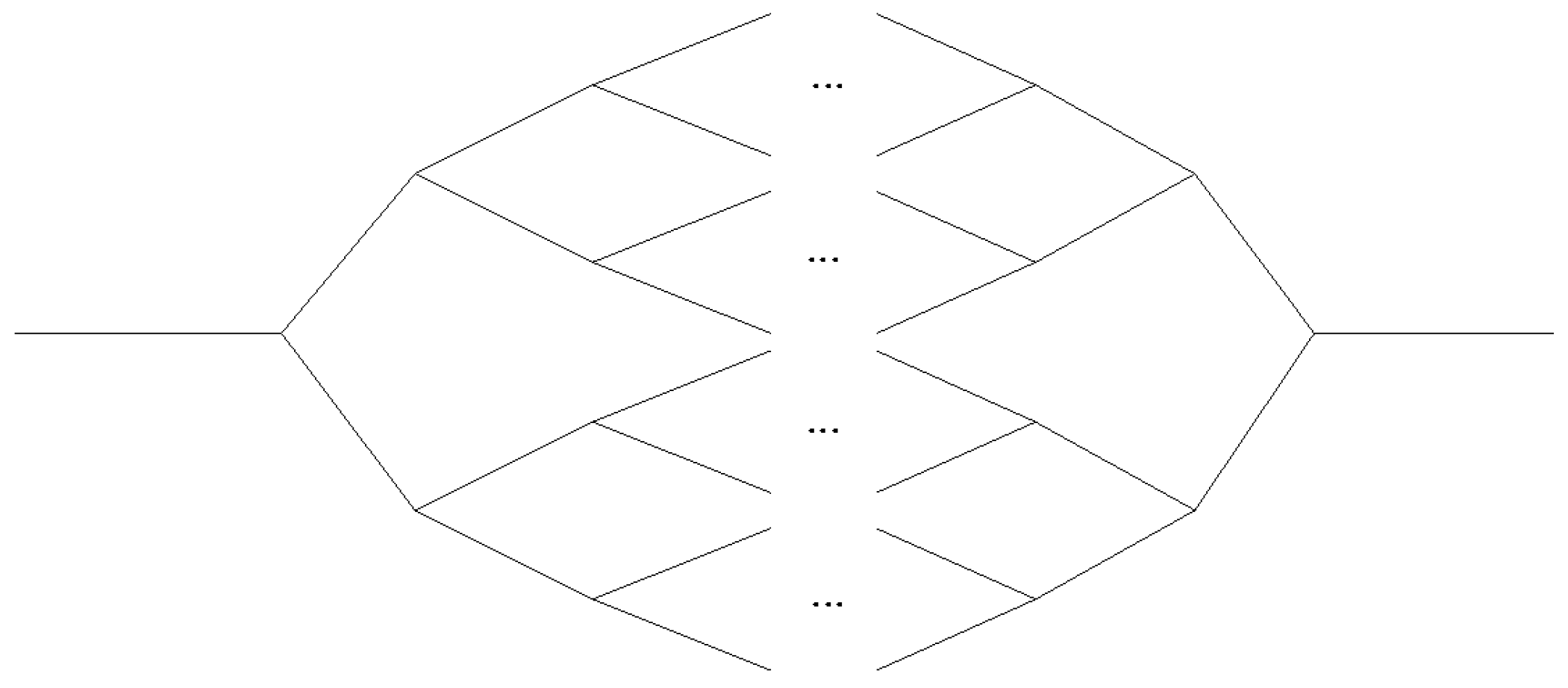We examine this connection with special attention to several unorthodox properties, such as, the extensivity of the q-entropy $S_q$ of fractal clusters of the order parameter and the anomalous (faster than exponential) sensitivity to initial conditions. A second example is that of the localization transition in electron transport in networks of scatterers. The use of a double Cayley tree model leads to an exact analogy with a nonlinear map that features two tangent bifurcations. 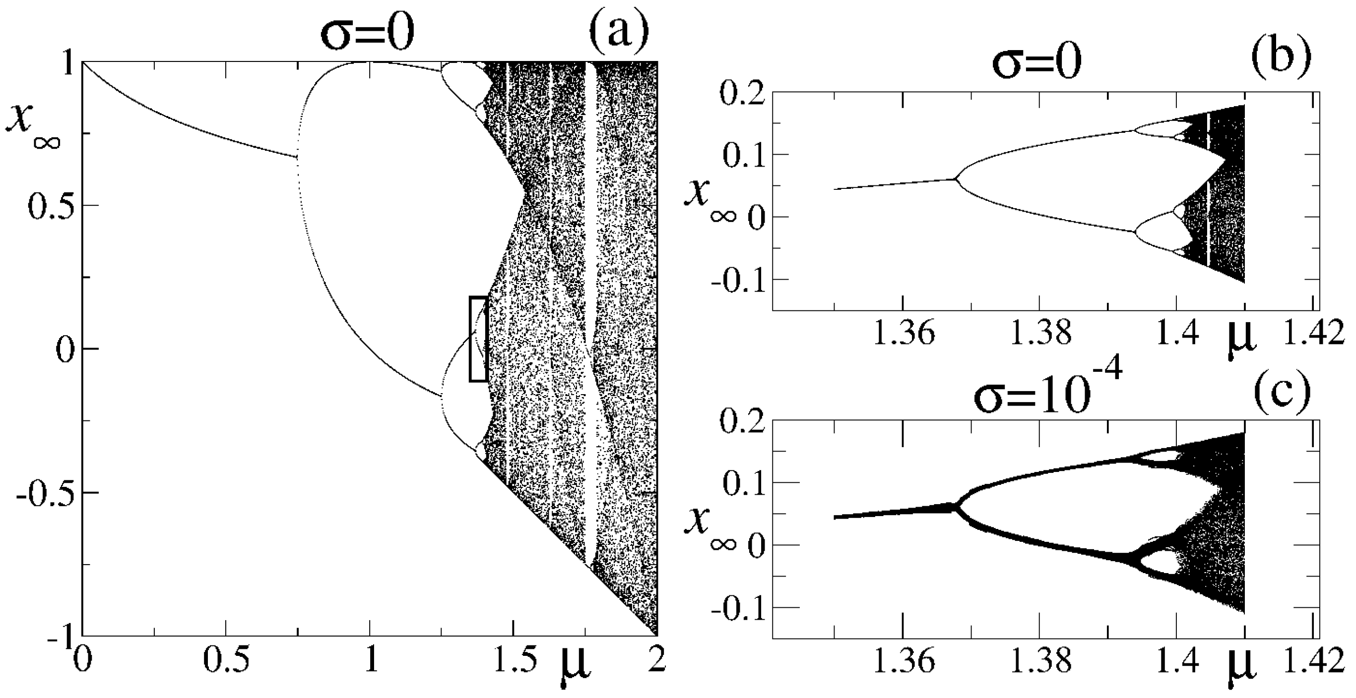The localization length is the inverse of the Lyapunov exponent, ${\lambda }_1$, and when this vanishes, we obtain a precise description of the mobility edge between insulating and conducting phases in terms of the q-generalized exponent, ${\lambda }_q$ [16]. 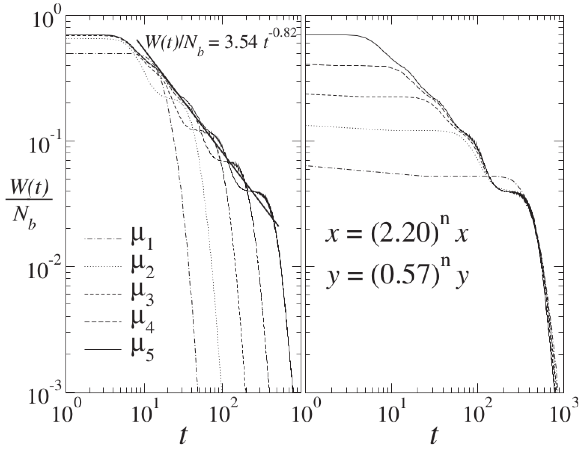As a third example, we describe our finding [17,18,19] that the dynamics at the noise-perturbed period-doubling onset of chaos is analogous to that observed in supercooled liquids close to vitrification. We have demonstrated that four major features of glassy dynamics in structural glass formers are displayed by orbits with a vanishing Lyapunov coefficient. These are: two-step relaxation, a relationship between relaxation time and configurational entropy, aging scaling properties and evolution from a diffusive regime to arrest. The known properties in control-parameter space of the noise-induced bifurcation gap in the period-doubling cascade [8] play a central role in determining the characteristics of dynamical relaxation at the chaos threshold.

The manifestations of q-statistics in complex systems of a general or interdisciplinary nature have been and are currently being exposed and established. Two illustrations of general nature are provided: one corresponds to dynamical hierarchies with modular organization and emergent properties. We recall the demonstration that the dynamics towards multifractal attractors as illustrated by the Feigenbaum point fulfills the main features of such dynamical hierarchies [20]. The other general topic is that of limit distributions of sums of deterministic variables, for which we describe and discuss the stationary distributions at the period-doubling transition to chaos and how they transform to Gaussian distributions for chaotic attractors. 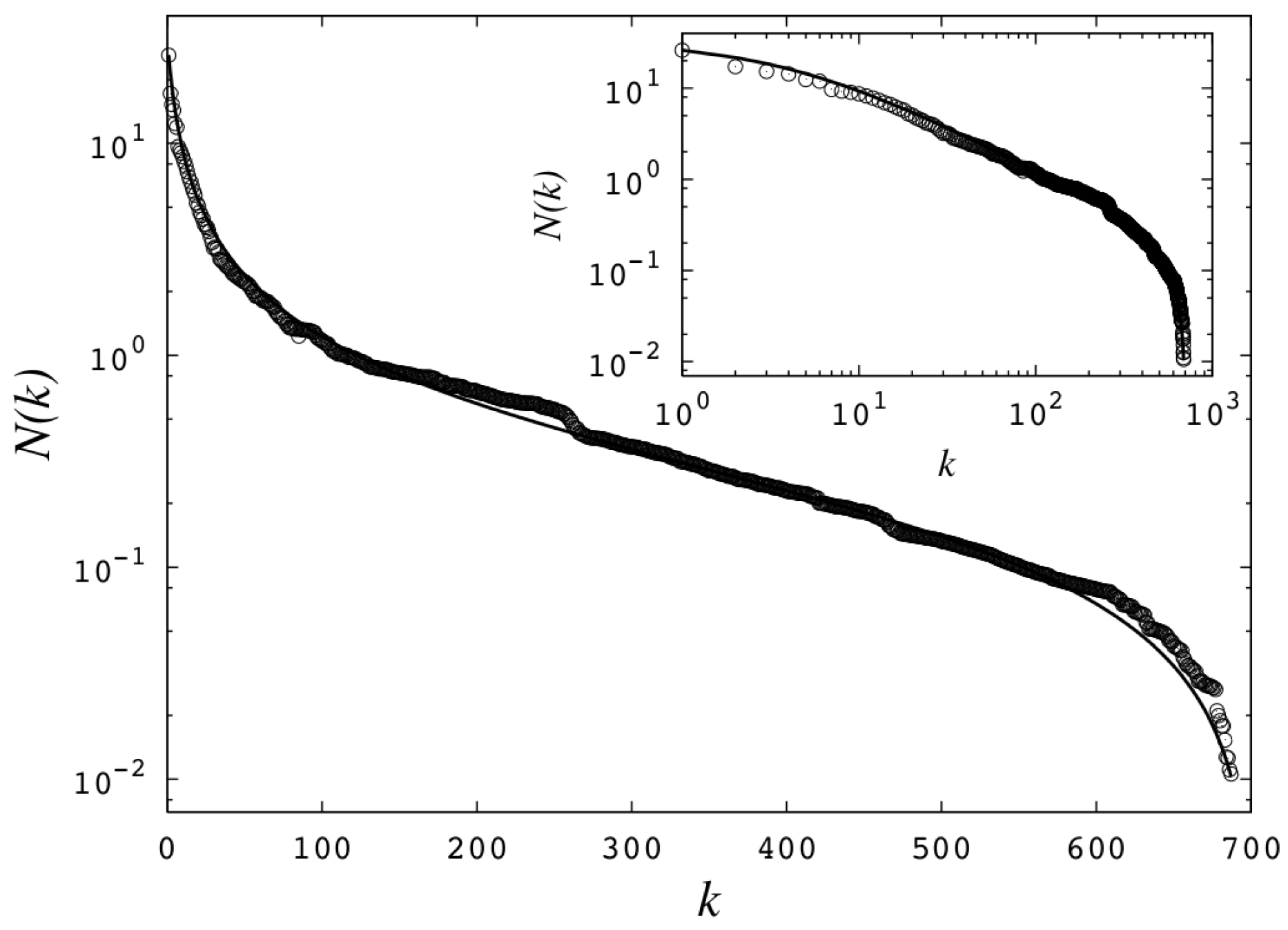We consider both cases, that of an initial trajectory inside the attractor and that of an ensemble of trajectories uniformly distributed throughout all of phase space [21,22,23]. We consider also two examples directed at more specific types of complex systems. One case corresponds to the large class of systems described by rank distributions. Their rank distributions are proved to be analogous to the dynamics at or near the tangent bifurcation [24]. Another set of studies correspond to the transcription of the time series formed by the trajectories generated by the critical attractors into networks via an appropriate algorithm known as the horizontal visibility method [25]. Generalized entropies play an important role in understanding these applications.

The structure of the rest of article is as follows: In Section 2, we provide the basic description of the anomalous dynamics at critical attractors that forms the core knowledge for the rest of the article. Of the three routes to chaos in one-dimensional nonlinear maps, we refer only to the intermittency and the period-doubling cases. For the sake of brevity, we do not provide a description of the quasiperiodic critical attractors and give only the relevant references. In Section 3, we extend our description to the intricate dynamics towards the Feigenbaum attractor and refer to its hierarchical structure with modular organization. In Section 4, we describe the stationary distributions produced by sums of positions in the dynamics associated with the Feigenbaum attractor and how they transform beyond the transition to chaos. In Section 5, we present our applications to condensed-matter complex systems, whereas in Section 6, we do so likewise for general or interdisciplinary complex systems. In Section 7, we discuss our results and make clarifying remarks.

2. Critical Attractors in Unimodal Maps

2.1. Two Different Routes to Chaos in Unimodal Maps

A unimodal map (a one-dimensional map with one extremum) contains infinite families of critical attractors with vanishing Lyapunov exponent ${\lambda }_1=0$ at which the ergodic and mixing properties breakdown [26]. These are the tangent bifurcations that give rise to windows of periodic trajectories within chaotic bands and the accumulation point(s) of the pitchfork bifurcations, the so-called period-doubling onset of chaos [8,9] at which these periodic windows come to an end. There are other attractors for which the Lyapunov exponent, ${\lambda }_1$, diverges to minus infinity, where there is faster than exponential convergence of orbits. These are the superstable attractors located between successive pitchfork bifurcations. They are present at the initial period-doubling cascade and at all the other cascades within periodic windows with accumulation points that are replicas of the Feigenbaum attractor.

The properties of the critical attractors are universal in the renormalization-group (RG) sense, that is, all maps, $f(x)$, that lead to the same fixed-point map, $f^{*}(x)$, under a repeated functional composition and rescaling transformation share the same scaling properties. For unimodal maps, this transformation takes the form $Rf(x)\equiv \alpha f(f(x/\alpha ))$, where α assumes a fixed value (positive or negative real number) for each universality class and $f^{*}(x)$ is given by:

$$f^{*}(x)\equiv \underset{n\to \infty }{lim}{R}^{(n)}f(x)=\underset{n\to \infty }{lim}{\alpha }^n{f}^{(2^n)}(x/{\alpha }^n)$$

(1)

and satisfies:

$$f^{*}(x)=\alpha f^{*}(f^{*}(x/\alpha ))$$

(2)

The universality of the static or geometrical properties of multifractal critical attractors has been understood since long ago [8,9]. This is represented, for example, by the generalized dimensions, $D_q$, or the spectrum, $f(\tilde{\alpha })$, that characterize the multifractal attractor at the period-doubling onset of chaos [1,9]. As we see below, the dynamical properties of critical attractors, multifractal or not, also display universality, the entropic index, q, in the sensitivity, ${\xi }_t$, and the Lyapunov spectra, ${\lambda }_q$, is given in terms of the universal constant, α. For the the pitchfork and tangent bifurcations, the results are relatively straightforward, but for the period-doubling accumulation point, the situation is more complex. In the latter case, an infinite set of universal constants, of which α is most prominent, is required. These constants are associated with the discontinuities off the trajectory scaling function, σ, that measures the convergence of positions in the orbits of period $2^n$ as $n\to \infty$ to the Feigenbaum attractor [8].

The sensitivity to initial conditions, ${\xi }_t$, is defined as:

$${\xi }_t(x_0)\equiv \underset{\Delta x_0\to 0}{lim}(\Delta x_t/\Delta x_0)$$

(3)

where $\Delta x_0$ is the initial separation of two orbits and $\Delta x_t$ that at time t. Notice, we do not write the customary limit, $t\gg 1$, above. As we shall see when ${\lambda }_1$ vanishes, ${\xi }_t$ has the form [3,27,28]:

$${\xi }_t(x_0)={exp}_q[{\lambda }_q(x_0)t]\equiv {[1-(q-1){\lambda }_q(x_0)t]}^{-1/(q-1)}$$

(4)

that yields the standard exponential, ${\xi }_t$, with ${\lambda }_1$, when $q\to 1$. In Equation (4), q is the entropic index and ${\lambda }_q$ is the q-generalized Lyapunov exponent; ${exp}_q(x)\equiv {[1-(q-1)x]}^{-1/(q-1)}$ is the q-exponential function. The local rate of entropy production, $K_1$, for chaotic attractors is given by $K_{1}t=S_1(t)-S_1(0)$ and $S_1=-{\sum }_i{p}_{i}ln{p}_i$ with $p_i$, the trajectories’ distribution. For chaotic attractors, the identity $K_1=$${\lambda }_1>0$ holds [9]. Notice that this is not the Pesin identity that, instead of $K_1$, employs the Kolmogorov–Sinai entropy, ${\mathcal{K}}_1$ [28]. For critical attractors, the identity still holds trivially, but a generalized form:

$$K_q={\lambda }_q$$

(5)

appears where the rate of q-entropy production, $K_q$, is defined via:

$$K_{q}t=S_q(t)-S_q(0)$$

(6)

and where:

$$S_q\equiv \sum _i{p}_i{ln}_q\left(\frac{1}{p_i}\right)=\frac{1-{\sum }_i^W{p}_i^q}{q-1}$$

(7)

is the Tsallis entropy (Recall that ${ln}_{q}y\equiv (y^{1-q}-1)/(1-q)$ is the functional inverse of ${exp}_q(y)$).

We take as a starting point and framework for the study of fixed-point map properties the prototypical logistic map, or its generalization to the non-linearity of order $\zeta >1$:

$$f_{\mu }(x)=1-\mu {\left|x\right|}^{\zeta },-1\le x\le 1,0\le \mu \le 2$$

(8)

where x is the phase space variable, μ the control parameter and $\zeta =2$ corresponds to the familiar logistic map. Our results relate to the anomalous ${\xi }_t$ and its associated spectrum, ${\lambda }_q$, for the above-mentioned critical attractors that are involved in the two routes to chaos exhibited by unimodal maps, the intermittency and the period doubling routes. For the Feigenbaum attractor, we describe the relationship of ${\xi }_t$ and ${\lambda }_q$ with Mori’s q-phase transitions [2,4].

2.2. Dynamics at the Tangent and Pitchfork Bifurcations

The exact fixed-point map solution of the RG Equation (2) for the tangent bifurcations, known since long ago [8,9], has been shown to describe the dynamics of iterates in the neighborhood of this attractor [3,29,30], as well. Furthermore, a straightforward extension of this approach was shown to apply to the pitchfork bifurcations [3,29,30]. We recall that period-doubling and intermittency transitions are based on the pitchfork and the tangent bifurcations, respectively, and that at these attractors, the ordinary Lyapunov coefficient ${\lambda }_1=0$. The sensitivity, ${\xi }_t$, can be determined analytically and its relation with the rate of entropy production examined [29,30]. The fixed-point expressions have the specific form that corresponds to the temporal evolution suggested by q -statistics. In [3,29,30] is contained the derivation of the q-Lyapunov coefficients, ${\lambda }_q$, and the description of the different possible types of sensitivity, ${\xi }_t$.

For the transition to periodicity of order n in the ζ-logistic map, the composition, $f_{\mu }^{(n)}$, is first considered. In the neighborhood of one of the n points tangent to the line with unit slope, one obtains:

$$f^{(n)}(x)=x+u{\left|x\right|}^z+o({\left|x\right|}^z)$$

(9)

where u is the expansion coefficient. At the tangent bifurcations, one has $z=2$ and $u>0$, whereas for the pitchfork bifurcations, one has instead $z=3$ , because $d^2{f}_{\mu }^{(2^k)}/d{x}^2=0$ at these transitions, and $u<0$ is now the coefficient associated with $d^3{f}_{\mu }^{(2^k)}/d{x}^3<0$.

The RG fixed-point map $x^{\prime }=f^{*}(x)$ associated with maps of the form in Equation (9) was found [31] to be:

$$x^{\prime }=x{exp}_z(u{x}^{z-1})=x{[1-(z-1)u{x}^{z-1}]}^{-1/(z-1)}$$

(10)

as it satisfies $f^{*}(f^{*}(x))={\alpha }^{-1}{f}^{*}(\alpha x)$ with $\alpha =2^{1/(z-1)}$ and has a power-series expansion in x that coincides with Equation (9) in the two lowest-order terms. (above $x^{z-1}\equiv {\left|x\right|}^{z-1}\mathrm{sgn}(x)$). The long time dynamics is readily derived from the static solution Equation (10); one obtains:

$${\xi }_t(x_0)={[1-(z-1)a{x}_0^{z-1}t]}^{-z/(z-1)},u=at$$

(11)

and so, $q=2-z^{-1}$ and ${\lambda }_q(x_0)=za{x}_0^{z-1}$ [3,4]. When $q>1$ the left-hand side ($x<0$) of the tangent bifurcation map, Equation (9) exhibits a weak insensitivity to initial conditions, i.e., power-law convergence of orbits. However at the right-hand side ($x>0$) of the bifurcation, the argument of the q-exponential becomes positive, and this results in a “super-strong” sensitivity to initial conditions, i.e., a sensitivity that grows faster than exponential [3]. For the tangent bifurcation, one has $z=2$ in $q=2-z^{-1}$, and so, $q=3/2$. For the pitchfork bifurcation, one has $z=3$ in $q=2-z^{-1}$, and one obtains $q=5/3$. Notably, these specific results for the index q are valid for all $\zeta >1$ and, therefore, define the existence of only two universality classes for unimodal maps, one for the tangent and the other one for the pitchfork bifurcations [3]. See Figure 1 and Figure 2 for numerical corroboration of the following. In Figure 1a, the full line is a linear regression, whose slope, $-31.15$, should be compared with the exact expression for the generalized Lyapunov exponent, which gives ${\lambda }_q=31.216\dots$ Inset: $|x_0^{-1}|{ln}_2(x_t/x_0)$, for $t=3m(m=1,2,\dots )$ and $x_0\sim -{10}^{-6}$. A linear regression gives, in this case, a slope of $-5.16$, to be compared with the exact result $u/3=5.203\dots$; In Figure 1b the full line is a linear regression with a slope equal to $31.22$. Inset: Log-linear plot of ${\xi }_t$ evidencing a super-exponential growth. In Figure 2 the full line is a linear regression, whose slope, $-2.55$, should be compared with the analytical expression for the generalized Lyapunov exponent, which gives ${\lambda }_q=-2.547\dots$ Inset: $x_0^{-2}{ln}_3(x_t/x_0)$, for $t=2m(m=1,2,\dots )$ and $x_0\sim +{10}^{-3}$. A linear regression gives, in this case, a slope of $-0.44$, to be compared with the analytical result $u/2=-0.424\dots$.

Figure 1. Numerical corroboration of Equation (11) for the tangent bifurcation. Panel (a) corresponds to the left side of the first tangent bifurcation for $\zeta =2$. Circles represent $|x_0^{-1}|{ln}_{\frac{3}{2}}({\xi }_t)$ for the iterates of $f^{(3)}$ and $x_0\sim -{10}^{-4}$. Panel (b) corresponds to the right side of the first tangent bifurcation for $\zeta =2$. Circles represent $|x_0^{-1}|{ln}_{\frac{3}{2}}({\xi }_t)$ for the iterates of $f^{(3)}$ and $x_0\sim +{10}^{-4}$. See text for description.

Figure 1. Numerical corroboration of Equation (11) for the tangent bifurcation. Panel (a) corresponds to the left side of the first tangent bifurcation for $\zeta =2$. Circles represent $|x_0^{-1}|{ln}_{\frac{3}{2}}({\xi }_t)$ for the iterates of $f^{(3)}$ and $x_0\sim -{10}^{-4}$. Panel (b) corresponds to the right side of the first tangent bifurcation for $\zeta =2$. Circles represent $|x_0^{-1}|{ln}_{\frac{3}{2}}({\xi }_t)$ for the iterates of $f^{(3)}$ and $x_0\sim +{10}^{-4}$. See text for description.

Figure 2. Numerical corroboration of Equation (11) for the first pitchfork bifurcation with $\zeta =1.75$. Circles represent $x_0^{-2}{ln}_{\frac{5}{3}}({\xi }_t)$ for the iterates of $f^{(2)}$ and $x_0\sim +{10}^{-3}$. See text for description.

Figure 2. Numerical corroboration of Equation (11) for the first pitchfork bifurcation with $\zeta =1.75$. Circles represent $x_0^{-2}{ln}_{\frac{5}{3}}({\xi }_t)$ for the iterates of $f^{(2)}$ and $x_0\sim +{10}^{-3}$. See text for description.

There is an interesting scaling property displayed by ${\xi }_t$ in Equation (11) similar to the scaling property known as aging in systems close to glass formation. This property is observed in two-time functions (e.g., time correlations) for which there is no time translation invariance, but scaling is observed in terms of a time ratio variable, $t/t_w$, where $t_w$ is a “waiting time” assigned to the time interval for the preparation or hold of the system before time evolution is observed through time t. This property can be seen immediately in ${\xi }_t$ if one assigns a waiting time, $t_w$, to the initial position, $x_0$, as $t_w=$$x_0^{1-z}$. Equation (11) reads now:

$${\xi }_{t,t_w}={[1-(z-1)at/t_w]}^{-z/(z-1)}$$

(12)

The sensitivity for this critical attractor is dependent on the initial position, $x_0$, or, equivalently, on its waiting time, $t_w$, the closer $x_0$ is to the point of tangency, the longer $t_w$, but the sensitivity of all trajectories fall on the same q-exponential curve when plotted against $t/t_w$. Aging has also been observed for the properties of the map in Equation ( 9), but in a different context [32].

Notice that our treatment of the tangent bifurcation differs from other studies of intermittency transitions [33] in that there is no feedback mechanism of iterates to indefinitely repeat the action of $f^{(n)}(x)$ or of its associated fixed-point map, $f^{*}(x)$. Therefore, impeded or incomplete mixing in phase space (a small interval neighborhood around $x=0$) arises from the special “tangency” shape of the map at the pitchfork and tangent transitions that produces monotonic trajectories. This has the effect of confining or expelling trajectories, causing anomalous phase-space sampling, in contrast to the thorough coverage in generic states with ${\lambda }_1>0$. By construction, the dynamics at the intermittency transitions describe a purely q-exponential regime.

2.3. Dynamics within the Period-Doubling Accumulation Point

The dynamics at the Feigenbaum attractor has been analyzed recently [4,27,34]. For the ζ-logistic map, this attractor is located at ${\mu }_{\infty }$, the accumulation point of the control parameter values for the pitchfork bifurcations, ${\mu }_n$, $n=1,2,\dots$, which is also that for the superstable orbits, ${\overline{\mu }}_n$, $n=1,2,\dots$. By taking as initial condition $x_0=0$ at ${\mu }_{\infty }$, or, equivalently, $x_1=1$, it is found that the resulting orbit, a superstable orbit of period $2^{\infty }$, consists of trajectories made of intertwined power laws that asymptotically reproduce the entire period-doubling cascade that occurs for $\mu <{\mu }_{\infty }$. This orbit captures the properties of the superstable orbits that precedes it. Here, again, the Lyapunov coefficient, ${\lambda }_1$, vanishes (although the attractor is also the limit of a sequence of supercycles with ${\lambda }_1\to -\infty$), and in its place, there appears a spectrum of q-Lyapunov coefficients, ${\lambda }_q^{(k)}$ (the k index is defined below). The dynamics within this attractor was originally studied in [2,35], and our interest has been to examine its properties in relation with the expressions of the Tsallis statistics. We found that the sensitivity to initial conditions has precisely the form of a set of interlaced q-exponentials, of which we determine the q-indexes and the associated ${\lambda }_q^{(k)}$. As mentioned, the appearance of a specific value for the q index (and actually, also, that for its conjugate value $Q=2-q$) turns out to be due to the occurrence of Mori’s “q-phase transitions” [2] between “local attractor structures” at ${\mu }_{\infty }$. Furthermore, it has also been shown [4,34] that the dynamical and entropic properties at ${\mu }_{\infty }$ are naturally linked through the q-exponential and q-logarithmic expressions, respectively, for the sensitivity to initial conditions, ${\xi }_t$, and for the entropy, $S_q$, in the rate of entropy production, $K_q^{(k)}$. We have analytically corroborated the equality ${\lambda }_q^{(k)}=$$K_q^{(k)}$. Our results support the validity of the q-generalized (local t) Pesin identity for critical attractors in low-dimensional maps.

More specifically, the absolute values for the positions $x_{\tau }$ of the trajectory with $x_{t=0}=0$ at time-shifted $\tau =t+1$ have a structure consisting of subsequences with a common power-law decay of the form ${\tau }^{-1/1-q}$ with:

$$q=1-ln2/(\zeta -1)ln\alpha (\zeta )$$

(13)

where $\alpha (\zeta )$ is the Feigenbaum universal constant for nonlinearity $\zeta >1$ that measures the period-doubling amplification of iterate positions [27]. That is, the Feigenbaum attractor can be decomposed into position subsequences generated by the time subsequences $\tau =(2k+1)2^n$, each obtained by proceeding through $n=0,1,2,\dots$ for a fixed value of $k=0,1,2,\dots$. See Figure 3.

Figure 3. Absolute values of positions in logarithmic scales of the first 1000 iterations τ for a trajectory of the logistic map at the onset of chaos ${\mu }_{\infty }$ with initial condition $x_0=0$. The numbers correspond to iteration times. The power-law decay of the time subsequences described in the text can be clearly appreciated.

Figure 3. Absolute values of positions in logarithmic scales of the first 1000 iterations τ for a trajectory of the logistic map at the onset of chaos ${\mu }_{\infty }$ with initial condition $x_0=0$. The numbers correspond to iteration times. The power-law decay of the time subsequences described in the text can be clearly appreciated.

The $k=0$ subsequence can be written as $x_t={exp}_{2-q}(-{\lambda }_q^{(0)}t)$ with ${\lambda }_q^{(0)}=(\zeta -1)ln\alpha (\zeta )/ln2$. These properties follow from the use of $x_0=0$ in the scaling relation [27]:

$$x_{\tau }\equiv \left|g^{{}^{(\tau )}}(x_0)\right|={\tau }^{-1/1-q}\left|g({\tau }^{1/1-q}{x}_0)\right|$$

(14)

where $g(x)$ is the Feigenbaum fixed-point map [8,9].

The sensitivity associated with trajectories with other starting points, $x_0\ne 0$, within the multifractal attractor (but located within either its most sparse or most crowded regions) can be determined similarly with the use of the time subsequences $\tau =(2k+1)2^n$. One obtains:

$${\lambda }_q^{(k)}=\frac{(\zeta -1)ln\alpha (\zeta )}{(2k+1)ln2}>0,k=0,1,2,\dots$$

(15)

for the positive branch of the Lyapunov spectrum, when the trajectories start at the most crowded ($x_{\tau =0}=1$) and finish at the most sparse ($x_{\tau =2^n}=0$) region of the attractor. By inverting the situation, we obtain:

$${\lambda }_Q^{(k)}=-\frac{2(\zeta -1)ln\alpha (\zeta )}{(2k+1)ln2}<0,k=0,1,2,\dots$$

(16)

for the negative branch of ${\lambda }_q^{(k)}$, i.e., starting at the most sparse ($x_{\tau =0}=0$) and finishing at the most crowded ($x_{\tau =2^n+1}=1$) region of the attractor. Notice that $Q=2-q$ as ${exp}_Q(y)=1/{exp}_q(-y)$. For the case $\zeta =2$, see [27,34]; for general $\zeta >1$ see [4], where, also, different and more direct derivations are presented. Therefore, when considering these two dominant families of orbits, all the q-Lyapunov coefficients appear associated with only two specific values of the Tsallis index, q and $2-q$, with q given by Equation (13). In Figure 4, we show the q-logarithm of ${\xi }_t(x_0=1)$ vs. t for the $k=0$ time subsequence $\tau =2^n$ when $\zeta =2$ and $q=1-ln2/ln\alpha (2)=0.2445\dots$ and ${\lambda }_q^{(0)}=ln\alpha (2)/ln2=1.3236\dots$.

Figure 4. The q-logarithm of sensitivity to initial conditions ${\xi }_t$ vs. t, with $q=1-ln2/ln\alpha =0.2445\dots$ and initial conditions $x_0=0$ and $x_0=\delta \simeq {10}^{-8}$ (circles). The full line is the linear regression, $y(t)$. As required, the numerical results reproduce a straight line with a slope very close to ${\lambda }_q=ln\alpha /ln2=1.3236\dots$

Figure 4. The q-logarithm of sensitivity to initial conditions ${\xi }_t$ vs. t, with $q=1-ln2/ln\alpha =0.2445\dots$ and initial conditions $x_0=0$ and $x_0=\delta \simeq {10}^{-8}$ (circles). The full line is the linear regression, $y(t)$. As required, the numerical results reproduce a straight line with a slope very close to ${\lambda }_q=ln\alpha /ln2=1.3236\dots$

Ensembles of trajectories with starting points close to $x_{\tau =0}=1$ expand in such a way that a uniform distribution of initial conditions remains uniform for all later times, $t\le T$, where T marks the crossover to an asymptotic regime. As a consequence of this, the identity of the rate of entropy production, $K_q^{(k)}$, with ${\lambda }_q^{(k)}$ was established [34]. See Figure 5 and Figure 6. A similar reasoning can be generalized to other starting positions [4].

Figure 5. Time evolution, in logarithmic scales, of a distribution, $p_i(\tau )$, of trajectories at ${\mu }_{\infty }$. Initial positions are contained within a cell adjacent to $x=1$, and i is the relative number of cells. Iteration time is shown for the first two subsequences ($k=0,1$).

Figure 5. Time evolution, in logarithmic scales, of a distribution, $p_i(\tau )$, of trajectories at ${\mu }_{\infty }$. Initial positions are contained within a cell adjacent to $x=1$, and i is the relative number of cells. Iteration time is shown for the first two subsequences ($k=0,1$).

Figure 6. Numerical corroboration (full circles) of the generalized Pesin identity $K_q^{(k)}={\lambda }_q^{(k)}$ at ${\mu }_{\infty }$. On the vertical axis, we plot the q-logarithm of ${\xi }_{t_k}$ (equal to ${\lambda }_q^{(k)}t)$ and in the horizontal axis $S_q$ (equal to $K_q^{(k)}t$). In both cases, $q=1-ln2/ln\alpha =0.2445\dots$ The dashed line is a linear fit. In the inset, the full lines are from analytical results.

Figure 6. Numerical corroboration (full circles) of the generalized Pesin identity $K_q^{(k)}={\lambda }_q^{(k)}$ at ${\mu }_{\infty }$. On the vertical axis, we plot the q-logarithm of ${\xi }_{t_k}$ (equal to ${\lambda }_q^{(k)}t)$ and in the horizontal axis $S_q$ (equal to $K_q^{(k)}t$). In both cases, $q=1-ln2/ln\alpha =0.2445\dots$ The dashed line is a linear fit. In the inset, the full lines are from analytical results.

Notably, the appearance of a specific value for the q index (and actually, also, that for its conjugate value $Q=2-q$) turns out [4] to be due to the occurrence of Mori’s “q-phase transitions” [2] between “local attractor structures” at ${\mu }_{\infty }$. To see this in more detail, we observe that the sensitivity, ${\xi }_t(x_0)$, can be obtained [4] from:

$${\xi }_t(m)\simeq {\left|\frac{{\sigma }_n(m-1)}{{\sigma }_n(m)}\right|}^n,t=2^n-1,n$$

(17)

where ${\sigma }_n(m)=d_{n+1,m}/d_{n,m}$ and where $d_{n,m}$ are the diameters that measure adjacent position distances that form the period-doubling cascade sequence [8]. Above, the choices, $\Delta x_0=d_{n,m}$ and $\Delta x_t=d_{n,m+t}$, $t=2^n-1$, have been made for the initial and the final separation of the trajectories, respectively. In the large n limit, ${\sigma }_n(m)$ develops discontinuities at each rational of the form $m/2^{n+1}$ [8], and according to the expression above for ${\xi }_t(m)$, the sensitivity is determined by these discontinuities. For each discontinuity of ${\sigma }_n(m)$, the sensitivity can be written in the forms [4]:

$${\xi }_t={exp}_q[{\lambda }_{q}t],{\lambda }_q>0$$

(18)

and:

$${\xi }_t={exp}_{2-q}[{\lambda }_{2-q}t],{\lambda }_{2-q}<0$$

(19)

where q and the spectra, ${\lambda }_q$ and ${\lambda }_{2-q}$, depend on the parameters that describe the discontinuity [4]. This result reflects the multi-region nature of the multifractal attractor and the memory retention of these regions in the dynamics. The pair of q -exponentials correspond to a departing position in one region and arrival at a different region and vice versa; the trajectories expand in one sense and contract in the other. The largest discontinuity of ${\sigma }_n(m)$ at $m=0$ is associated with trajectories that start and finish at the most crowded ($x\simeq 1$) and the most sparse ($x\simeq 0$) regions of the attractor. In this case, one obtains, again, Equation (15), the positive branch of the Lyapunov spectrum, when the trajectories start at $x\simeq 1$ and finish at $x\simeq 0$. By inverting the situation, one obtains Equation (16), the negative branch of the Lyapunov spectrum. Therefore, when considering these two dominant families of orbits, all the q-Lyapunov coefficients appear associated with only two specific values of the Tsallis index, q and $Q=2-q$, with q given by Equation (13).

As a function of the running variable $-\infty <\mathsf{q}<\infty$, the q -Lyapunov coefficients become a function, $\lambda (\mathsf{q})$, with two steps located at $\mathsf{q}=q=1-ln2/(\zeta -1)ln\alpha (\zeta )$ and $\mathsf{q}=Q=2-q$. See Figure 7. In this manner, contact can be established with the formalism developed by Mori and coworkers [2] and the q-phase transition obtained numerically in [35,36]. The step function for $\lambda (\mathsf{q})$ can be integrated to obtain the spectrum of local coefficients, $\varphi (\mathsf{q})$ ($\lambda (\mathsf{q})\equiv d\varphi /d\lambda (\mathsf{q})$), and its Legendre transform, $\psi (\lambda )$ ($\equiv \varphi -(1-\mathsf{q})\lambda$), the dynamic counterparts of the Renyi dimensions, $D(\mathsf{q})$, and the spectrum of local dimensions, $f(\tilde{\alpha })$, that characterize the geometry of the attractor. The result for $\psi (\lambda )$ is:

$$\psi (\lambda )=\left\{\begin{array}{c}(1-Q)\lambda ,{\lambda }_Q^{(0)}<\lambda <0\hfill \\ (1-q)\lambda ,0<\lambda <{\lambda }_q^{(0)}\hfill \end{array}\right.$$

(20)

As with ordinary thermal first order phase transitions, a q-phase transition is indicated by a section of linear slope $1-q$ in the spectrum (free energy), $\psi (\lambda )$, a discontinuity at q in the Lyapunov function (order parameter), $\lambda (\mathsf{q})$, and a divergence at q in the variance (susceptibility), $v(\mathsf{q})$. For the onset of chaos at ${\mu }_{\infty }(\zeta =2)$, a q-phase transition was determined numerically [2,35,36]. According to $\psi (\lambda )$ above, we obtain a conjugate pair of q-phase transitions that correspond to trajectories linking two regions of the attractor, the most crowded and most sparse. See Figure 7. Details appear in [4]. See [6] for the derivation of the analog expressions for ${\xi }_t$, ${\lambda }_q^{(k)}$, $K_q^{(k)}$, $\lambda (\mathsf{q})$ and $\psi (\lambda )$ associated with the dynamics at the quasiperiodic critical attractor via the golden ratio route to chaos in the circle map.

Figure 7. (a) The Lyapunov coefficient function, $\lambda (q)$, at the chaos threshold at ${\mu }_{\infty }$; and (b) the spectrum, $\psi (\lambda )$. See the text for a description.

Figure 7. (a) The Lyapunov coefficient function, $\lambda (q)$, at the chaos threshold at ${\mu }_{\infty }$; and (b) the spectrum, $\psi (\lambda )$. See the text for a description.

3. Dynamics towards the Feigenbaum Attractor

3.1. Diameters, Repellors and Gap Formation

The knowledge of the dynamics towards a particular family of periodic attractors, the so-called superstable attractors [8,9], facilitates the understanding of the rate of approach of trajectories to the Feigenbaum attractor, located at $\mu ={\mu }_{\infty }$, and highlights the source of the discrete scale invariant property of this rate [5]. The family of trajectories associated with these attractors (also called supercycles) of periods $2^N$, $N=1,2,3,\dots$, are located along the bifurcation forks. The positions (or phases) of the $2^N$-attractor are given by $x_j=f_{{\overline{\mu }}_N}^{(j)}(0)$, $j=1,2,\dots ,2^N$. Notice that infinitely many other sequences of superstable attractors appear at the period-doubling cascades within the windows of periodic attractors for values of $\mu >$${\mu }_{\infty }$. Associated with the $2^N$-attractor at $\mu ={\overline{\mu }}_N$, there is a $(2^N-1)$-repellor consisting of $2^N-1$ positions $y_k$, $k=0,1,2,\dots ,2^N-1$. These positions are the unstable solutions, $\left|d{f}_{{\overline{\mu }}_N}^{(2^{n-1})}(y)/dy\right|>1$, of $y=f_{{\overline{\mu }}_N}^{(2^{n-1})}(y)$, $n=1,2,\dots ,N$. The first, $n=1$, originates at the initial period-doubling bifurcation; the next two, $n=2$, start at the second bifurcation, and so on, with the last group of $2^{N-1}$, $n=N$, setting out from the $N-1$ bifurcation. The diameters, $d_{N,m}$, are defined as $d_{N,m}\equiv x_m-f_{{\overline{\mu }}_N}^{(2^{N-1})}(x_m)$.

Central to our understanding of the dynamical properties of unimodal maps is the following in-depth property: Time evolution at ${\mu }_{\infty }$ from $\tau =0$ up to $\tau \to \infty$ traces the period-doubling cascade progression from $\mu =0$ up to ${\mu }_{\infty }$. There is an underlying quantitative relationship between the two developments. Specifically, the trajectory inside the Feigenbaum attractor with initial condition $x_0=0$, the $2^{\infty }$-supercycle orbit, takes positions $x_{\tau }$, such that the distances between appropriate pairs of them reproduce the diameters, $d_{N,m}$, defined from the supercycle orbits with ${\overline{\mu }}_N<{\mu }_{\infty }$. See Figure 8, where the absolute value of positions and logarithmic scales are used to illustrate the equivalence. This property has been basic in obtaining rigorous results for the sensitivity to initial conditions for the Feigenbaum attractor [4] and for the dynamics of approach to this attractor [5]. Other families of periodic attractors share most of the properties of supercycles. Below, we consider explicitly the case of a map with a quadratic maximum, but the results are easily extended to general nonlinearity $\zeta >1$.

Figure 8. (Left panel) Absolute value of attractor positions for the logistic map, $f_{\mu }(x)$ , in logarithmic scale, as a function of $-ln{(\mu )}_{\infty }-\mu$. (Right panel) Absolute value of trajectory positions for $f_{\mu }(x)$ at ${\mu }_{\infty }$ with initial condition $x_0=0$ in logarithmic scale, as a function of the logarithm of time τ; τ is also shown by the numbers close to the diamonds. The arrows indicate the equivalence between the diameters $d_{N,0}$ in the left panel and position differences ${\delta }_n$ with respect to $x_0=0$ in the right panel.

Figure 8. (Left panel) Absolute value of attractor positions for the logistic map, $f_{\mu }(x)$ , in logarithmic scale, as a function of $-ln{(\mu )}_{\infty }-\mu$. (Right panel) Absolute value of trajectory positions for $f_{\mu }(x)$ at ${\mu }_{\infty }$ with initial condition $x_0=0$ in logarithmic scale, as a function of the logarithm of time τ; τ is also shown by the numbers close to the diamonds. The arrows indicate the equivalence between the diameters $d_{N,0}$ in the left panel and position differences ${\delta }_n$ with respect to $x_0=0$ in the right panel.

The organization of the total set of trajectories as generated by all possible initial conditions as they flow towards a period, $2^N$, attractor has been determined in detail [5,37]. It was found that the paths taken by the full set of trajectories in their way to the supercycle attractors (or to their complementary repellors) are exceptionally structured. The dynamics associated with families of trajectories always displays a characteristically concerted order in which positions are visited, and this is reflected in the dynamics of the supercycles of periods $2^N$ via the successive formation of gaps in phase space (the interval $-1\le x\le 1$) that finally give rise to the attractor and repellor multifractal sets. See Figure 9. To observe explicitly this process, an ensemble of initial conditions, $x_0$, distributed uniformly across phase space, was considered, and their positions were recorded at subsequent times [5,37]. This set of gaps develops in time, beginning with the largest one associated with the first repellor position, then followed by a set of two gaps associated with the next two repellor positions; next, a set of four gaps associated with the four next repellor positions, and so forth. The gaps that form consecutively all have the same width in the logarithmic scales (see Figure 14, Figure 15, Figure 16 and Figure 17 in [5]), and therefore, their actual widths decrease as a power law, the same power law followed, for instance, by the position sequence $x_{\tau }={\alpha }^{-N}$, $\tau =2^N$, $N=0,1,2,\dots$ for the trajectory inside the attractor starting at $x_0=0$ (and where $\alpha \simeq 2.50291$ is the absolute value of Feigenbaum’s universal constant for $\zeta =2$). The locations of this specific family of consecutive gaps (the largest gaps for each value of k) advance monotonically toward the sparsest region of the multifractal attractor located at $x=0$. See [5,37] for more details.

3.2. Sums of Diameters as Partition Functions

The rate of convergence, $W_t$, of an ensemble of trajectories towards any attractor/repellor pair along the period-doubling cascade is a convenient single-time quantity that has a straightforward definition and is practical to implement numerically. A partition of phase space is made of $N_b$ equally-sized boxes or bins, and a uniform distribution of $N_c$ initial conditions is placed along the interval, $-1\le x\le 1$. The ratio, $N_c/N_b$, can be adjusted to achieve optimal numerical results [5]. The quantity of interest is the number of boxes, $W_t$, that contain trajectories at time t. This rate has been determined for the supercycles ${\overline{\mu }}_N$, $N=1,2,3,\dots$ and its accumulation point ${\mu }_{\infty }$ [5]. See Figure 10, where $W_t$ is shown in logarithmic scales for the first five supercycles of periods $2^1$ to $2^5$, where we can observe the following features: In all cases, $W_t$ shows a similar initial and nearly constant plateau $W_t\simeq \Delta$, $1\le t\le t_0$, $t_0=O(1)$, and a final well-defined decay to zero. The jump Δ at ${\mu }_{\infty }$ is $\Delta =(1+{\alpha }^{-1})/2\simeq 0.69977$, due to the fact that all initial conditions out of the interval ($-{\alpha }^{-1}$,1) take a value inside this interval after the first iteration. As can be observed in the left panel of Figure 10, the time position of the final decay grows approximately proportionally to the period $2^N$ of the supercycle. There is an intermediate slow decay of $W_t$ that develops as N increases with duration, also just about proportional to $2^N$. For the shortest period, $2^1$, there is no intermediate feature in $W_t$; this appears first for period $2^2$ as a single dip and expands with one undulation every time N increases by one unit. The expanding intermediate regime exhibits the development of a power-law decay with logarithmic oscillations (characteristic of discrete scale invariance). In the limit, $N\to \infty$, the rate takes the form $W_t\simeq \Delta h(ln\tau /ln2){\tau }^{-\varphi }$, $\tau =t-t_0$, where $h(x)$ is a periodic function with $h(1)=1$ and $\varphi \simeq 0.8001$ [5].

Figure 9. Phase-space gap formation for $\mu ={\mu }_3$. (Left panel) Time evolution of a uniform ensemble of ${10}^4$ trajectories as a function of $|x|$ (black areas and open circles). The values of the index k label the order of the gap set. (Right panel) Rotated plots of $f_{{\overline{\mu }}_3}^{(8)}(x)$ and as guides for the identification of attractor and repellor positions.

Figure 9. Phase-space gap formation for $\mu ={\mu }_3$. (Left panel) Time evolution of a uniform ensemble of ${10}^4$ trajectories as a function of $|x|$ (black areas and open circles). The values of the index k label the order of the gap set. (Right panel) Rotated plots of $f_{{\overline{\mu }}_3}^{(8)}(x)$ and as guides for the identification of attractor and repellor positions.

The rate, $W_t$, at the values of time for period doubling, $\tau =2^n$, $n=1,2,3,\dots <N$, can be obtained quantitatively from the supercycle diameters $d_{n,m}$. Specifically:

$$Z_{\tau }\equiv \frac{W_t}{\Delta }=\sum _{m=0}^{2^{n-1}-1}{d}_{n,m},\tau =t-t_0=2^{n-1},n=1,2,3,\dots <N$$

(21)

Equation (21) expresses the numerical procedure followed in [38] to evaluate the exponent, ϕ, but it also suggests a statistical-mechanical structure if $Z_{\tau }$ is identified as a partition function, where the diameters, $d_{n,m}$, play the role of configurational terms [5]. The diameters, $d_{N,m}$, scale with N for m fixed as $d_{N,m}\simeq {\alpha }_y^{-(N-1)}$, N large, where the ${\alpha }_y$ are universal constants obtained from the finite discontinuities of Feigenbaum’s trajectory scaling function $\sigma (y)={lim}_{N\to \infty }(d_{N,m+1}/d_{N,m})$, $y={lim}_{N\to \infty }(m/2^N)$ [5,8]. The largest two discontinuities of $\sigma (y)$ correspond to the sparsest and denser regions of the multifractal attractor at ${\mu }_{\infty }$, for which we have, respectively, $d_{N,0}\simeq {\alpha }^{-(N-1)}$ and $d_{N,1}\simeq {\alpha }^{-2(N-1)}$ ($d_{1,0}=1$). The diameters, $d_{N,m}$, can be rewritten exactly as q-exponentials via use of the identity $A^{-(N+1)}\equiv {(1+\beta )}^{-lnA/ln2}$, $\beta =2^{N-1}-1$. That is, $d_{N,m}\simeq {exp}_{q_y}(-\beta {ϵ}_y)$, where, $q_y=1-{ϵ}_y^{-1}$, ${ϵ}_y=-ln{\alpha }_y/ln2$, and $\beta =\tau -1=2^{N-1}-1$. Similarly, $Z_{\tau }\simeq {\tau }^{-\varphi }$ can be expressed as $Z_{\tau }\simeq {exp}_{\mathcal{Q}}(-\beta \varphi )$, where $\mathcal{Q}=1-{\varphi }^{-1}$. Therefore, taking the above into account in Equation (21), we have:

$${exp}_{\mathcal{Q}}(-\beta \varphi )\simeq \sum _y{exp}_{q_y}(-\beta {ϵ}_y)$$

(22)

Equation (22) resembles a basic statistical-mechanical expression with the exception that q-deformed exponential weights appear in place of ordinary exponential weights (that are recovered when $\mathcal{Q}=q_y=1$). We emphasize that the left- and right-hand sides in Equations (21) and (22) are given by quantities that describe the dynamics of approach and within the attractor, respectively. See [5,39] for related details.

Figure 10. (Left panel) Rate $W_t$, divided by the number of boxes, $N_b$, employed, of an approach to the attractor for the supercycles of periods $2^N,N=1,2,3,4$ and 5 on logarithmic scales. The expression shown corresponds to the power law decay of the developing logarithmic oscillations. Right panel: Superposition of the five curves for $W_t$ in the left panel via n-times repeated rescaling factors shown for the horizontal x and vertical y axes.

Figure 10. (Left panel) Rate $W_t$, divided by the number of boxes, $N_b$, employed, of an approach to the attractor for the supercycles of periods $2^N,N=1,2,3,4$ and 5 on logarithmic scales. The expression shown corresponds to the power law decay of the developing logarithmic oscillations. Right panel: Superposition of the five curves for $W_t$ in the left panel via n-times repeated rescaling factors shown for the horizontal x and vertical y axes.

3.3. Dynamical Hierarchies with Modular Organization

We point out [20] that it is possible to generate hierarchical systems with dynamical organization from a formal starting point in the form of a simple closed-form nonlinear dynamical system. Furthermore, that nonlinear dynamics tuned at the transition to chaos can lead to an emergent property. We illustrate this standpoint by appropriate interpretation to the properties of the dynamics towards the Feigenbaum attractor we are discussing.

3.3.1. Preimage Structure and Flow of Trajectories towards the Attractor

The organization of the total set of trajectories as generated by all possible initial conditions as they flow towards a period $2^N$ attractor is described in [5,37]. It was found that the paths taken by the full set of trajectories on their way to the supercycle attractors (or to their complementary repellors) are exceptionally structured. We define the preimage, $x^{(k)}$, of order k of position x to satisfy $x=h^{(k)}(x^{(k)})$, where $h^{(k)}(x)$ is the k-th composition of the map, $h(x)\equiv f_{{\overline{\mu }}_N}^{(2^{N-1})}(x)$. The preimages of the attractor of period $2^N$, $N=1,2,3,\dots$, are distributed into different basins of attraction, one for each of the $2^N$ phases (positions) that composes the cycle. When $N\ge 2$, these basins are separated by fractal boundaries, whose complexity increases with increasing N. The boundaries consist of the preimages of the corresponding repellor and their positions cluster around the $2^N-1$ repellor positions, according to an exponential law. As N increases, the structure of the basin boundaries becomes more involved. Namely, the boundaries for the $2^N$ cycle develops new features around those of the previous $2^{N-1}$ cycle boundaries, with the outcome that a hierarchical structure arises, leading to embedded clusters of clusters of boundary positions, and so forth. The dynamics associated with families of trajectories always displays a characteristically concerted order in which positions are visited, which, in turn, reflects the repellor preimage boundary structure of the basins of attraction. That is, each trajectory has an initial position that is identified as a preimage of a given order of an attractor (or repellor) position, and this trajectory necessarily follows the steps of other trajectories, with the initial conditions of lower preimage order belonging to a given chain or pathway to the attractor (or repellor). When the period $2^N$ of the cycle increases, the dynamics becomes more involved with increasingly more complex stages that reflect the hierarchical structure of preimages. See Figure 11 and Figure 12, and see [5,37] for details. The fractal features of the boundaries between the basins of attraction of the positions of the periodic orbits develop a structure with hierarchy, and this, in turn, echoes in the properties of the trajectories. The set of trajectories produce an ordered flow towards the attractor or towards the repellor that follows through the ladder structure of the sub-basins that constitute the mentioned boundaries.

From our previous discussion, we know that, every time the period of a supercycle increases from $2^{N-1}$ to $2^N$ by a shift in the control parameter value from ${\overline{\mu }}_{N-1}$ to ${\overline{\mu }}_N$, the preimage structure advances one stage of complication in its hierarchy. Along with this, and in relation to the time evolution of the ensemble of trajectories, an additional set of $2^N$ smaller phase-space gaps develops, and, also, a further oscillation takes place in the corresponding rate, $W_t$, for finite period attractors. At ${\mu }_{\infty }$, the time evolution tracks the period-doubling cascade progression, and every time t increases from $2^{N-1}$ to $2^N$, the flow of trajectories undergoes equivalent passages across stages in the itinerary through the preimage ladder structure, in the development of phase-space gaps and in logarithmic oscillations in $W_t$. Thus, each doubling of the period introduces additional modules or building blocks in the hierarchy of the preimage structure, such that the complexity of these added modules is similar to that of the total period $2^N$ system. As a consequence of this, we have obtained detailed understanding of the mechanism by means of which the discrete scale invariance implied by the log-periodic property [5] in the rate of approach $W_t$ arises.

Figure 11. (Top panel) Time of flight $t_f(x)$ for $N=2$; the black lines correspond to initial conditions that terminate at the attractor positions $x=0$ and $x\simeq -0.310703$ and the gray lines to trajectories ending at $x=1$ and $x\simeq 0.8734$. (Right (left) bottom panel) Same as the top panel, but plotted against the logarithm of $x-y_1(y_1-x)$. It is evident that the peaks are arranged exponentially around the old repellor position, $y_1$, i.e., they appear equidistant on a logarithmic scale.

Figure 11. (Top panel) Time of flight $t_f(x)$ for $N=2$; the black lines correspond to initial conditions that terminate at the attractor positions $x=0$ and $x\simeq -0.310703$ and the gray lines to trajectories ending at $x=1$ and $x\simeq 0.8734$. (Right (left) bottom panel) Same as the top panel, but plotted against the logarithm of $x-y_1(y_1-x)$. It is evident that the peaks are arranged exponentially around the old repellor position, $y_1$, i.e., they appear equidistant on a logarithmic scale.

Figure 12. Same as Figure 11, but for $N=3$. The black lines correspond to initial conditions that terminate at any of the four attractor positions close or equal to $x=0$ and the gray lines to trajectories ending at any of the other four attractor positions close or equal to $x=1$. As the bottom panels show, on a logarithmic scale, in this case, there are (infinitely) many clusters of peaks (repellor preimages) equidistant from each other

Figure 12. Same as Figure 11, but for $N=3$. The black lines correspond to initial conditions that terminate at any of the four attractor positions close or equal to $x=0$ and the gray lines to trajectories ending at any of the other four attractor positions close or equal to $x=1$. As the bottom panels show, on a logarithmic scale, in this case, there are (infinitely) many clusters of peaks (repellor preimages) equidistant from each other

3.3.2. Dynamical Hierarchy

We proceed now to the identification of the features of the dynamics towards the Feigenbaum attractor as those of a bona fide model of dynamical hierarchy with modular organization. These are: (i) elementary degrees of freedom and the elementary events associated with them; (ii) building blocks and the dynamics that takes place within them and through adjacent levels of blocks; (iii) self-similarity characterized by coarse graining and renormalization-group (RG) operations; and (iv) the emerging property of the entire hierarchy absent in the embedded building blocks.

The elementary degrees of freedom are the preimages of the attractors of period $2^N$. These are assigned an order k, according to the number k of map iterations they require to reach the attractor. The preimages are also distinguished in relation to the position, $x_1$, …, $x_{2^N}$, of the attractor they reach first. The preimages of each attractor position appear grouped in basins with fractal boundaries. The elementary dynamical event is the reduction of the order k of a preimage by one unit. This event is generated by a single iteration of the map for an initial position placed in a given basin. The result is the translation of the position to a neighboring basin of the same attractor position.

The building blocks are clusters of clusters formed by families of boundary basins. The (boundary) basins of attraction of the $2^N$ positions of the periodic attractors cluster exponentially and have an alternating structure [5,37]. In turn, these clusters cluster exponentially themselves with their own alternating structure. Furthermore, there are clusters of these clusters of clusters with similar arrangements, and so on. The dynamics associated with the building blocks consists of the flow of preimages through and out of a cluster or block. Sets of preimages “evenly” distributed (say, one per boundary basin) across a cluster of order N (generated by an attractor of period $2^N$) flow orderly throughout the structure. If there is one preimage in each boundary basin of the cluster, each map iteration produces a migration from boundary basin to boundary basin in such a way that, at all times, there is one preimage per boundary basin, except for the inner ones in the cluster that are gradually emptied.

The self-similar feature in the hierarchy is demonstrated by the coarse-graining property amongst building blocks of the hierarchy that leaves the hierarchy invariant when $\mu ={\mu }_{\infty }$. That is, clusters of order N can be simplified into clusters of order $N-1$. There is a self-similar structure for the clusters of any order, and a coarse graining can be performed on clusters of order N, such that these can be reduced to clusters of a lower order; the basic coarse graining is to transform order N into order $N-1$. Furthermore, coarse graining can be carried out effectively via the RG functional composition and rescaling, as this transformation reduces the order N of the periodic attractor. Automatically, the building-block structure simplifies into that of the next lower order, and the clusters of boundary basins of preimages are reduced in one unit of involvedness. Dynamically, the coarse-graining property appears as flow within a cluster of order N simplified into flow within a cluster of order $N-1$. As coarse graining is performed in a given cluster structure of order N, the flow of trajectories through it is correspondingly coarse grained. e.g., flow out of a cluster of clusters is simplified as flow out of a single cluster. RG transformation via functional composition and rescaling of the cluster flow is displayed dynamically, since by definition functional composition establishes the dynamics of iterates, and the RG transformation $Rf(x)=-\alpha f(f(-x/\alpha )$ leads, for N finite, to a trivial fixed point that represents the simplest dynamical behavior, that of the period one attractor. For $N\to \infty$, the RG transformation leads to the self-similar dynamics of the non-trivial fixed point, the period-doubling accumulation point.

There is a modular structure of embedded clusters of all orders. The building blocks, clusters of order N, form well-defined sets that are embedded into larger building blocks, sets of clusters of order $N+1$. As the period $2^N$ of the attractor that generates this structure increases, the hierarchy extends, and as N diverges, a fully self-similar structure develops. The RG transformation for $N\to \infty$ no longer reduces the order of the clusters, and a nontrivial fixed point arises. The trajectories consist of embedded flows within clusters of all orders. The entire flow towards the $2^N$-period attractor generated by an ensemble of initial conditions (distributed uniformly across the phase space interval of the map) methodically follows a pattern predetermined by the hierarchical structure of embedded clusters of the preimages.

Each module exhibits a basic kind of flow property. This is the exponential emptying of trajectories within a cluster of order N. Trajectories initiated in the boundary basins that form a cluster of order N flow out of it with an iteration time exponential law. The flow is transferred into a cluster of order $N+1$. This flow is a dynamical module from which a structure of flows is composed. The emerging property that appears when $N\to \infty$ is that there is a power-law emptying of trajectories for the entire hierarchy. The flow of trajectories towards an attractor of period $2^N$ proceeds via a sequence of stage or step flows, each within a cluster of a given order. Thus, the first is through a cluster of order one, then through a cluster of order two, etc., until the last stage is through a cluster of order N. The sequence evolves in time via a power law decay that is modulated by logarithmic oscillations. This is the emerging property of the model.

4. Distributions of Sums of Deterministic Variables

The limit distributions of sums of deterministic variables at the period-doubling transition to chaos in unimodal maps have been studied by making use of the trajectory properties described above [21,22]. Firstly, the sum of positions as they are visited by a single internal trajectory was found to have a multifractal structure imprinted by that of the critical attractor [21,22]. It was shown, analytically and numerically, that the sum of values of positions display discrete scale invariance fixed jointly by Feigenbaum’s universal constant, α, and by the period doublings contained in the number of summands. The stationary distribution associated with this sum has a multifractal support given by the Feigenbaum attractor. Secondly, the sum of subsequent positions generated by an ensemble of uniformly distributed initial conditions in the entire phase space was determined [23]. It was found that this sum acquires features of the repellor preimage structure that dominates the dynamics toward the attractor. The stationary distribution associated with this ensemble has a hierarchical structure with multifractal and discrete scale invariance properties.

4.1. Sums of Positions of a Single Trajectory within the Attractor

The starting point is the numerical evaluation of the sum of absolute values, $\left|x_t\right|$, at ${\mu }_{\infty }$ and with $x_0=0$:

$$y(N)\equiv \sum _{t=1}^N\left|x_t\right|$$

(23)

Figure 13 shows the result, where it can be observed that the values recorded, besides a repeating fluctuating pattern within a narrow band, increase linearly on the whole. The measured slope of the linear growth is $c=0.56245\dots$. The top inset shows an enlargement of the band, where some detail of the complex pattern of values of $y(N)$ is observed. A stationary view of the mentioned pattern is shown in bottom inset, where we plot

$$y^{\prime }(N)\equiv \sum _{t=1}^N\left(\left|x_t\right|-c\right)$$

(24)

in logarithmic scales. There, we observe that the values of $y^{\prime }(N)$ fall within horizontal bands interspersed by gaps, revealing a fractal or multifractal set layout. The top (zeroth) band contains $y^{\prime }$ for all the odd values of N; the first band next to the top band contains $y^{\prime }$ for the even values of N of the form $N=2+4m$, $m=0,1,2,\dots$. The second band next to the top band contains $y^{\prime }(N)$ for $N=2^2+2^{3}m$, $m=0,1,2,\dots$, and so on. In general, the k-th band next to the top band contains $y^{\prime }(2^k+2^{k+1}m)$, $m=0,1,2,\dots$. Another important feature in this figure inset is that the $y^{\prime }(N)$ for subsequences of N each of the form $N=(2l+1)2^k$, $k=0,1,2,\dots$, with l fixed at a given value of $l=0,1,2,\dots$, appear aligned with a uniform slope $s=-1.323\dots$ (See the dotted line linking the values of $y^{\prime }(N)$ when $l=0$). The parallel lines formed by these subsequences imply the power law $y^{\prime }(N)\sim N^s$ for N belonging to such a subsequence.

Figure 13. Sum of absolute values of visited points, $x_t,t=0,\dots ,N$, of the Feigenbaums attractor with initial condition $x_0=0$. Top inset: a closer look of the path of the sum, for values of N ranging between 35 and 50. Bottom inset: Centered sum $y^{\prime }(N)$ in logarithmic scales. See the text.

Figure 13. Sum of absolute values of visited points, $x_t,t=0,\dots ,N$, of the Feigenbaums attractor with initial condition $x_0=0$. Top inset: a closer look of the path of the sum, for values of N ranging between 35 and 50. Bottom inset: Centered sum $y^{\prime }(N)$ in logarithmic scales. See the text.

We have seen [4] that these two characteristics of $y^{\prime }(N)$ are also present in the layout of the absolute value of the individual positions $\left|x_t\right|$, $t=1,2,3,\dots$ of the trajectory initiated at $x_0=0$; and this layout corresponds to the multifractal geometric configuration of the points of the Feigenbaum’s attractor; see Figure 3. In this case, the horizontal bands of positions separated by equally-sized gaps are related to the period-doubling diameters, $d_{n,m}$, that are used to construct the multifractal attractor. The identical slope shown in the logarithmic scales by all the position subsequences $\left|x_t\right|$, $t=(2l+1)2^k$, $k=0,1,2,\dots$, each formed by a fixed value of $l=0,1,2,\dots$, implies the power law $\left|x_t\right|\sim t^s$, $s=-ln\alpha /ln2=-1.3236\dots$, as the $\left|x_t\right|$ can be expressed as:

$$\left|x_t\right|\simeq \left|x_{2l+1}\right|{\alpha }^{-k}$$

(25)

$t=(2l+1)2^k$, $k=0,1,2,\dots$, or, equivalently, $\left|x_t\right|\sim t^s$. Notice that the index k also labels the order of the bands from top to bottom. The power law behavior involving the universal constant, α, of the subsequence positions reflect the approach of points in the attractor toward its most sparse region at $x=0$ from its most compact region, as the positions at odd times $\left|x_{2l+1}\right|=x_{2l+1}$, those in the top band, correspond to the densest region of the set. Having uncovered the manifestation of the multifractal structure of the attractor into the sum, $y^{\prime }(N)$, it is possible to proceed to derive Equations (23) and (24) analytically [21,22] and to corroborate that the value of the slope, s, in Figure 13 is indeed given by $s=-ln\alpha /ln2=-1.3236\dots$. The derivation also illustrates the discrete scale invariant property of the time evolution at the period doubling transition to chaos. That is, a duplication in iteration time is accompanied by a scale factor in the iterate position equal to the universal constant, α.

In [21,22], the next step was to consider the straight sum of $x_t$, where the signs taken by positions lessen the growth of its value as N increases, and the results found were consistently similar to those for the sum of $\left|x_t\right|$, i.e., the linear growth of a fixed-width band within which the sum displays a fluctuating arrangement. Numerical and analytical details for the sum of $x_t$ are described in detail in [21,22]. After this, numerical results for the sum of iterated positions obtained when the control parameter is shifted into the region of chaotic bands were obtained. In all of these cases, the distributions evolve after a characteristic crossover towards a Gaussian form. These findings were explained in terms of an RG framework in which the action of the central limit theorem plays a fundamental role and provide details of the crossover from multiband distributions to the Gaussian distribution [21,22].

4.2. Sums of Positions of an Ensemble of Trajectories Evolving towards the Attractor

A second, different, but complementary, study [23] consists of the evaluation of the sum of positions, $x_t$, up to a final iteration time, N, of a trajectory with initial condition $x_0$ and control parameter value μ, i.e.,:

$$X(x_0,N;\mu )\equiv \sum _{t=0}^N{x}_t$$

(26)

Figure 14 shows the results for $X(x_0,N;{\mu }_{\infty }$ for all possible initial conditions, $-1\le x_0\le 1$ and $N\sim O({10}^6)$. The plot is symmetrical with respect to $x_0=0$ and exhibits two large peaks and a central valley. This provides the main frame onto which motifs of alternating signs and diminishing amplitude are added consecutively. The distribution associated with the set of sums, $X(x_0,N;{\mu }_{\infty }$, is shown in Figure 15, which we observe has an asymmetrical double exponential global shape with superposed motifs of ever-decreasing finer detail characteristic of a multifractal object. The dynamical properties described above of trajectories as they evolve towards the Feigenbaum attractor can be used to explain the dynamical origin of all the features of this distribution. Bearing in mind the basic property that trajectories at ${\mu }_{\infty }$ from $t=0$ up to $t\to \infty$ trace the period-doubling cascade progression from $\mu =0$ up to ${\mu }_{\infty }$, it is clear now how to decode the structure of the sums in Figure 14 and that of its histogram in Figure 15. As explained in [23], the arrangement of the multiscale families of cusps of $X(x_0,N;{\mu }_{\infty })$ is the manifestation of the consecutive formation of phase space gaps in an initially uniform distribution of positions $x_0$ and the logarithmic oscillations at times $t^k$, $k=1,2,3,\dots$ of the rate of convergence of trajectories $W_t$ to the Feigenbaum attractor. The mean time for the opening of gaps of the same order is $t^k$, $k=1,2,3,\dots$, and the signs and amplitudes of the cusps are the testimonies stamped in the sums of the main passages out of the labyrinths formed by the preimages of the repellor, the transits of trajectories from one level of the hierarchy to the next. Visual representation of the stationary distribution, $P(X,N\to \infty ;{\mu }_{\infty })$, associated with the sums, $X(x_0,N;{\mu }_{\infty })$, is shown by the histogram in Figure 15. It has an asymmetrical double exponential backbone onto which multiscale patterns are attached that originate from the aforementioned sets of cusps in the sums. The negative slope (in semi-logarithmic scales) of the backbone originates from the main $k=1$ repellor core structure shown for all supercycles, while the steeper positive slope originated form the replica structures of the former that originate from the $k=2$ repellor structures.

Figure 14. Sums $X(x_0,N;{\mu }_{\infty })$ as a function of $x_0$, $N\sim O({10}^6)$ at the Feigenbaum point.

Figure 14. Sums $X(x_0,N;{\mu }_{\infty })$ as a function of $x_0$, $N\sim O({10}^6)$ at the Feigenbaum point.

Figure 15. Histograms obtained from the sums in Figure 14. The inset shows greater detail.

Figure 15. Histograms obtained from the sums in Figure 14. The inset shows greater detail.

We have found that the sum of iterate positions within the Feigenbaum’s attractor has a multifractal structure stamped by that of the attractor, while that involving positions of an ensemble of trajectories moving toward the attractor exhibits the preimage structure of its corresponding repellor. These basic features suggest a degree of universality, limited to the critical attractor under consideration, in the properties of sums of deterministic variables at the transitions to chaos. Namely, the sums of positions of memory-retaining trajectories evolving under a vanishing Lyapunov exponent appear to preserve the particular features of the multifractal critical attractor and repellor under examination. Thus, we expect that varying the degree of nonlinearity of a unimodal map would affect the scaling properties of time averages of trajectory positions at the period doubling transition to chaos, or alternatively, that the consideration of a different route to chaos, such as the quasiperiodic route, would lead to different scaling properties of comparable time averages. Furthermore, as commented on above, the spiked functional dependence of the sums $X(x_0,N;{\mu }_{\infty })$ on $x_0$ shown in Figure 14 follows the characteristic hierarchical preimage structure, with exponential clustering, around the positions of the major and other high ranking elements of the repellor and their first preimages [5]. This feature suggests that the distribution of large sums of positions is dominated by long journeys toward the attractor that are particular to the critical attractor under consideration.

5. Manifestations of Incipient Chaos in Condensed Matter Systems

It is of interest to know if the anomalous dynamics found for critical attractors in low-dimensional maps bears some correlation with the anomalous dynamical behavior at extremal or transitional states in systems with many degrees of freedom characteristic of condensed matter physics. Three specific examples have been developed. In one case, the dynamics at the tangent bifurcation has been shown to be related to that of evanescent fluctuations, or order parameter clusters, at thermal critical states [14,15]. The second case also involves the tangent bifurcation and appears in a description of the localization transition between a conducting and an insulating phase [16]. In the third case, the dynamics at the period-doubling onset of chaos has been demonstrated to be closely analogous to the glassy dynamics observed in supercooled molecular liquids [17,18,19].

5.1. Critical Clusters

We examine first the intermittent properties of clusters of the order parameter at critical thermal states [14,15]. Our interest is in the local fluctuations of a system undergoing a second order phase transition, for example, in the Ising model as the magnetization fluctuates and generates magnetic domains on all size scales at its critical point. In particular, the object of study is a single cluster of order parameter ϕ at criticality. This is described by a coarse-grained free energy or effective action, like in the Landau–Ginzburg–Wilson (LGW) continuous spin model portrayal of the equilibrium configurations of Ising spins at the critical temperature and zero external field. At criticality, the LGW free energy takes the form:

$${\Psi }_c[\varphi ]=a\int d{r}^d\left[\frac{1}{2}{\left(\nabla \varphi \right)}^2+b{\left|\varphi \right|}^{\delta +1}\right]$$

(27)

Where a and b are constants, δ is the critical isotherm exponent and d is the spatial dimension ($\delta =5$ for the $d=3$ Ising model with short range interactions). As we describe below, a cluster of radius R is an unstable configuration whose amplitude in ϕ grows in time and eventually collapses when an instability is reached. This process has been shown [12,13] to be reproduced by a nonlinear map with tangency and feedback characteristics, such that the time evolution of the cluster is given in the nonlinear system as a laminar event of intermittent dynamics.

The method employed to determine the cluster’s order parameter profile, $\varphi (\mathbf{r})$, adopts the saddle-point approximation of the coarse-grained partition function, Z, so that $\varphi (\mathbf{r})$ is its dominant configuration and is determined by solving the corresponding Euler–Lagrange equation. The procedure is equivalent to the density functional approach for stationary states in equilibrium nonuniform fluids. Interesting properties have been derived from the thermal average of the solution found for $\varphi (\mathbf{r})$, evaluated by integrating over its amplitude, ${\varphi }_0$, the remaining degree of freedom after its size, R, has been fixed. These are the fractal dimension of the cluster [40,41] and the intermittent behavior in its time evolution [12,13]. Both types of properties are given in terms of the critical isotherm exponent, δ.

As we describe below, the dominance of $\varphi (\mathbf{r})$ in Z depends on a condition that can be expressed as an inequality between two lengths in space. This is $r_0\gg R$, where $r_0$ is the location of a divergence in the expression for $\varphi (\mathbf{r})$ that decreases as an inverse power of the cluster amplitude, ${\varphi }_0$. When $r_0\gg R$, the profile is almost horizontal, but for $r_0⪆R$, the profile increases from its center faster than an exponential. This is responsible for the cluster properties described in [14,15]. These properties relate to the dependence of the number of cluster configurations on size R and the sensitivity to initial conditions ${\xi }_t$ of the order-parameter evolution on time t. When the method considers a one dimensional system with unspecified range of interactions, the magnetization profile turns out exactly to have the form of a q-exponential:

$$\varphi (x)={\varphi }_0{exp}_q(kx)$$

(28)

with $q=$$(1+\delta )/2$ and $k=\sqrt{2b}{\varphi }_0^{(\delta -1)/2}$ [14,15]. Because $\delta >1$, one has $q>1$, and $\varphi (x)$ grows faster than an exponential as $x\to x_0$ and diverges at $x_0$. It is important to notice that only configurations with $R\ll x_0$ have a nonvanishing contribution to the path integration in Z and that these configurations vanish for the infinite cluster-sized system. There are some characteristics of nonuniform convergence in relation to the limits, $R\to \infty$ and $x_0\to \infty$, a feature that is significant for our connection with q-statistics. By taking $\delta =1$, the system is set out of criticality; then, $q=1$, and the profile, $\varphi (x)$, becomes the exponential $\varphi (x)={\varphi }_{0}exp(k_{0}x)$, $k_0=\sqrt{a_{0}t}$. The analysis can be carried out for higher dimensions with no further significant assumptions and with comparable results [12,13,40,41].

The total magnetization of the cluster of size R (see Figure 16):

$$\Phi (R)={\int }_0^{R}dx\varphi (x)={\Phi }_0\{{[{exp}_q(kR)]}^{2-q}-1\},R<x_0$$

(29)

can be used to estimate its entropy rate of growth with R [14,15], and it is significant to note that this rate has the form of the Tsallis entropy and complies with the extensivity property, $S_q\sim R$, while the BG entropy obtained from $S_q$ when $q=1$ complies also with the extensivity property, $S_1\sim R$ [14,15]. That is, $S_q$ is extensive only at criticality, and the BG $S_1$ is extensive only off criticality. A condition for these properties associated with $S_q$, $q>1$, to arise is criticality, but also is the situation that phase space has only been partially represented by selecting configurations that are dominant only under certain conditions. Hence, the motivation to examine this problem rests on explaining the physical and methodological basis under which proposed generalizations of the BG statistics may apply.

Figure 16. Total magnetization of the cluster, $\Phi (R)$, as a function of the cluster size, R, according to Equation (29) for $q=2$ and 3, which correspond, respectively, to $\delta =3$ and 5.

Figure 16. Total magnetization of the cluster, $\Phi (R)$, as a function of the cluster size, R, according to Equation (29) for $q=2$ and 3, which correspond, respectively, to $\delta =3$ and 5.

5.2. Mobility Edge

We refer now to a remarkable equivalence between the dynamics of an intermittent nonlinear map and the electronic transport properties (obtained via the scattering matrix approach) of a crystal defined on a double Cayley tree [16]. See Figure 17. This analogy is strict [16] and reveals in detail the nature of the mobility edge normally studied near, but not at, the metal-insulator transition in disordered systems. An analytical expression for the conductance that has a q-exponential form was obtained as a function of system size at this transition. This manifests as power-law decay or fast variability according to different kinds of boundary conditions. The model does not contain disorder; nevertheless, it displays a transition between localized and extended states. The translation of the map dynamical expressions into electronic transport terms provides not only the description of two different conducting phases, but offered a rigorous account of the conductance at the mobility edge [16]. A new type of localization length in the incipient insulator mirrors the departure from exponential sensitivity to initial conditions at the transition to chaos.

Figure 17. A double Cayley tree of connectivity $K=2$ and lattice constant a. Each bond is a perfect one-dimensional conductor.

Figure 17. A double Cayley tree of connectivity $K=2$ and lattice constant a. Each bond is a perfect one-dimensional conductor.

The recursion formula for scattering matrices corresponding to consecutive sizes was reduced to a nonlinear map, where time iterations represent increments in size. The number of times the trees are ramified, starting from the perfect wire or lead, is the generation, n, that quantifies the size of the system. For brevity, the tree connectivity was fixed to $K=2$, where one lead, the incoming lead, is divided into two outgoing leads at a given node. Basic to the discussion is the fact that the scattering matrix recursive relation can be written in a diagonal form, and this implies the existence of a one-dimensional nonlinear map for the electronic phase, ${\theta }_n$. The map ${\theta }_{n+1}=f({\theta }_n)$ was obtained in the following closed form [16]:

$$f({\theta }_n)=2ka-{\theta }_n+2arctan\left(\frac{sin{\theta }_n+\sqrt{1-2ϵ}sin2ka}{cos{\theta }_n-\sqrt{1-2ϵ}cos2ka}\right)$$

(30)

where the dependence on the transmission probability, ϵ, the k momentum and the lattice constant, a, comes out explicitly. Figure 18 illustrates the map in Equation (30) for different parameter values.

Figure 18. $f({\theta }_n)$ of Equation (30), for $ϵ=\frac{1}{4}$: (a) $ka=\pi /4$ (dashed), $2\pi /4$ (long dashed), $3\pi /4$ (continuous); and (b) $ka=2.6$ (long dashed), $3\pi /4$ (continuous), 2.1 (dashed). The dotted lines correspond to the identity.

Figure 18. $f({\theta }_n)$ of Equation (30), for $ϵ=\frac{1}{4}$: (a) $ka=\pi /4$ (dashed), $2\pi /4$ (long dashed), $3\pi /4$ (continuous); and (b) $ka=2.6$ (long dashed), $3\pi /4$ (continuous), 2.1 (dashed). The dotted lines correspond to the identity.

The dynamical properties of the map given by Equation (30) translate into the following network properties: (i) There are two families of period one attractors for small and large values of $ka$ separated by a family of chaotic attractors for intermediate values of $ka$. For fixed ϵ, these families are connected by tangent bifurcation points at $k_{c}a$ and $k_c^{\prime }a$. (ii) In relation to the attractors of period one that take place along $0\le ka<k_{c}a$ and $k_c^{\prime }a<ka\le \pi$, it was found that the ordinary Lyapunov exponent, ${\lambda }_1$, is negative, and therefore, the conductance, $g_n$, decays exponentially with system size n,$g_n=exp(2{\lambda }_{1}n)$, implying localization, the localization length being ${\zeta }_1=a/|{\lambda }_1|$. In Figure 19a, we see a clear exponential decay of $g_n$ as a function of n at $ka=0.5$, where we compare $g_n$ computed directly with that obtained from ${\lambda }_1$. (iii) With respect to the chaotic attractors that occur in the interval, $k_{c}a<ka<k_c^{\prime }a$, it was observed that ${\lambda }_1$ becomes positive, and the recursion relation does not let $g_n$ decay, but makes it oscillate with n (not shown here), indicating that conduction takes place. In our model, $g_n$ does not scale with system size as in the metallic regime of quasi-one-dimensional disordered wire, where Ohm’s law is satisfied. In the parameter region where the map is incipiently chaotic, say $ka\gtrsim k_{c}a$, the network grows with n with an insulator character, but interrupted for other intermediate values of n by conducting crystals. In the map dynamics, these are the laminar episodes separated by chaotic bursts in intermittent trajectories.

Figure 19. Conductance as a function of generation for $ϵ=\frac{1}{4}$, (a) $ka=0.5$ and (b) $ka=\pi /4$. Continuous lines represent $g_n$ obtained directly from the map through Equation (30), while dotted lines correspond to $g_n=exp(2{\lambda }_{1}n)$ and $g_n={exp}_{3/2}(2{\lambda }_{3/2}n)$ for panels (a) and (b), respectively. The two curves in (b) differ because of a proportionality factor; see Equation (32).

Figure 19. Conductance as a function of generation for $ϵ=\frac{1}{4}$, (a) $ka=0.5$ and (b) $ka=\pi /4$. Continuous lines represent $g_n$ obtained directly from the map through Equation (30), while dotted lines correspond to $g_n=exp(2{\lambda }_{1}n)$ and $g_n={exp}_{3/2}(2{\lambda }_{3/2}n)$ for panels (a) and (b), respectively. The two curves in (b) differ because of a proportionality factor; see Equation (32).

The most distinct outcome of the treatment in [16] is the description obtained of the mobility edge from the dynamics at the critical points located at $ka=k_c^{\prime }a$ and $ka=k_{c}a$. There, ${\zeta }_1=a/|{\lambda }_1|\to \infty$, and not much can be said about the size dependence of the conductance when $n\gg 1$. However, we can use to our advantage the known properties of the anomalous dynamics occurring at these transitions once they are identified as tangent bifurcations (see Figure 19b for $ka=3\pi /4$). As we have seen, at a tangent bifurcation of general nonlinearity $z>1$, the sensitivity obeys a q-exponential law for large n [3]:

$${\xi }_n={exp}_q({\lambda }_{q}n)\equiv {[1-(q-1){\lambda }_{q}n]}^{\mp \frac{1}{q-1}}$$

(31)

where ${\lambda }_q$ is a q-generalized Lyapunov coefficient given by ${\lambda }_q=\mp zu$, $q=2-1/z$, where u is the leading term of the expansion up to order z of ${\theta }_n$ close to ${\theta }_c$ (or ${\theta }_c^{\prime }$); i.e., ${\theta }_n-{\theta }_c=({\theta }_{n-1}-{\theta }_c)+u{|{\theta }_{n-1}-{\theta }_c|}^z+\cdots$. The minus and plus signs in Equation (31) and in ${\lambda }_q$ correspond to trajectories at the left and right, respectively, of the point of tangency, ${\theta }_c$. Equation (31) implies the power-law decay of ${\xi }_n$ with n when ${\theta }_n-{\theta }_c<0$ and faster than exponential growth when ${\theta }_n-{\theta }_c>0$. By making the expansion around ${\theta }_c$ (or ${\theta }_c^{\prime }$) for map Equation (30), it was found (as anticipated) $z=2$, implying $q=3/2$, and $u=\sqrt{(1-2ϵ)/2ϵ}$. The conductance $g_n$ at each bifurcation point acquires the form $g_n={exp}_{3/2}(2{\lambda }_{3/2}n)$ [16], or:

$$g_n\propto {\left(1-\frac{1}{2}{\lambda }_{3/2}n\right)}^{-4}$$

(32)

where the q-generalized Lyapunov exponent is ${\lambda }_{3/2}=-2\sqrt{1-2ϵ/2ϵ}<0$. In the right panel of Figure 19b, results are compared for the conductance obtained from Equation (32) (dashed line) and that obtained from the Landauer formula [16]. It is clear that $g_n$ decays as a power law (with quartic exponent) rather than the exponential in the insulating phase. We emphasize that a localization length given by ${\zeta }_{3/2}=a/{\lambda }_{3/2}$ can still be defined at the mobility edge. When ${\theta }_n-{\theta }_c>0$, ${\lambda }_{3/2}=2\sqrt{1-2ϵ/2ϵ}>0$ and the recursion relation for $g_n$ describes an incipient conductor with exceptionally fast fluctuating $g_n$.

In summary, we can draw significant conclusions about electronic transport from the study in [16]. These arise naturally when considering the dynamical properties of the equivalent nonlinear map near or at the intermittency transition to chaos. Since iteration time in the map translates into the generation, n, of the network, time evolution means the growth of system size, reaching the thermodynamic limit (and true self-similarity) when $n\to \infty$. In that limit, windows of period one separated by a chaotic band correspond, respectively, to localized and extended electronic states. Further, in the referred parameter ($ka$, ϵ) regions, the conductance, $g_n$, of the model crystal shows either an exponential decay with system size, with localization length given by ${\zeta }_1=1/|{\lambda }_1|$ (as in the case of a quasi-one-dimensional disordered wire), or a fluctuating property, signaling conducting states. The pair of tangent bifurcation points of the map correspond to the band or mobility edges that separate conductor from insulator behavior. At these bifurcations, the sensitivity to initial conditions, ${\xi }_n$, exhibits either power-law decay (when ${\theta }_0<{\theta }_c^{\prime }$ or ${\theta }_0>{\theta }_c$) or faster than exponential increase (${\theta }_c^{\prime }<{\theta }_0<{\theta }_c$), and consequently, the conductance inherits comparable decay or variability with system size n. Notably, at the mobility edge, it is still possible to define a localization length, the q-generalized localization, length ${\zeta }_q=1/|{\lambda }_q|$, with a fixed value of $q=3/2$. This expression is universal, i.e., it is satisfied by all maps that in the neighborhood of the point of tangency have a quadratic term, i.e., $z=2$ [3].

5.3. Glassy Dynamics

A third example of a link between critical attractors and condensed-matter systems properties is the realization [17,18,19] that the dynamics at the noise-perturbed period-doubling onset of chaos in unimodal maps is analogous to that observed in supercooled liquids close to vitrification. Four major features of glassy dynamics in structural glass formers, two-step relaxation, aging, a relationship between relaxation time and configurational entropy, and evolution from diffusive behavior to arrest, are shown to be displayed by the properties of orbits with a vanishing Lyapunov coefficient. The previously known properties in control-parameter space of the noise-induced bifurcation gap [8,42] play a central role in determining the characteristics of dynamical relaxation at the chaos threshold.

A very pronounced slowing down of relaxation processes is the principal expression of the approach to the glass transition [43,44], and this is generally interpreted as a progressively more imperfect realization of phase space sampling. Because of this extreme condition, an important question is to find out whether, under conditions of ergodicity and mixing breakdown, the BG statistical mechanics remains capable of describing stationary states in the immediate vicinity of glass formation.

The basic ingredient of ergodicity failure is obtained for orbits at the onset of chaos (at ${\mu }_{\infty }$ for unimodal maps) in the limit towards vanishing noise amplitude. Our study supports the idea of a degree of universality underlying the phenomenon of vitrification and points out that it is present in different classes of systems, including some with no explicit consideration of their molecular structure. The map has only one degree of freedom, but the consideration of external noise could be taken to be the effect of many other systems coupled to it, like in the so-called coupled map lattices [45]. Our interest has been to study a system that is gradually forced into a non-ergodic state by reducing its capacity to sample regions of its phase space that are space filling, up to a point at which it is only possible to move within a multifractal subset of this space. The logistic map with additive external noise reads:

$$x_{t+1}=f_{\mu }(x_t)=1-\mu x_t^2+\sigma {\chi }_t,-1\le x_t\le 1,0\le \mu \le 2$$

(33)

where ${\chi }_t$ is a Gaussian-distributed random variable with average $〈{\chi }_t{\chi }_{t^{\prime }}〉={\delta }_{t.t^{\prime }}$, and σ measures the noise intensity [8,42].

The erratic motion of a Brownian particle is usually described by the Langevin theory [46]. As is well known, this method finds a way to avoid the detailed consideration of many degrees of freedom by representing with a noise source the effect of collisions with molecules in the fluid in which the particle moves. The approach to thermal equilibrium is produced by random forces, and these are sufficient to determine dynamical correlations, diffusion and a basic form for the fluctuation-dissipation theorem [46]. In the same spirit, attractors of nonlinear low-dimensional maps under the effect of external noise can be used to model states in systems with many degrees of freedom. Notice that the general map formula:

$$x_{t+1}=x_t+h_{\mu }(x_t)+\sigma {\chi }_t$$

(34)

is a discrete form for a Langevin equation with the nonlinear “friction force” term, $h_{\mu }$, and ${\chi }_t$ is the same Gaussian white noise random variable as in Equation (33) and σ, the noise intensity. With the choice $h_{\mu }(x)=1-x-\mu x^2$, we recover Equation (33).

5.3.1. Noise-Perturbed Onset of Chaos

When $\sigma >0$, the noise fluctuations smear the fine structure of the periodic attractors as the iterate visits positions within a set of bands or segments, like those in the chaotic attractors (see Figure 20); however, there is still a distinct transition to chaos at ${\mu }_{\infty }(\sigma )$, where the Lyapunov exponent, ${\lambda }_1$, changes sign. The period doubling of bands ends at a finite maximum period $2^{N(\sigma )}$ as $\mu \to {\mu }_{\infty }(\sigma )$ and then decreases at the other side of the transition. This effect displays scaling features and is referred to as the bifurcation gap [8,42]. When σ is small, the trajectories sequentially visit the set of $2^{N(\sigma )}$ disjoint bands, leading to a cycle, but the behavior inside each band is chaotic. The trajectories represent ergodic states as the accessible positions have a fractal dimension equal to the dimension of phase space. When $\sigma =0$, the trajectories correspond to a non-ergodic state, since as $t\to \infty$, the positions form only a multifractal set of fractal dimension $d_f=0.5338\dots$. Thus the removal of the noise, $\sigma \to 0$, leads to an ergodic to non-ergodic transition in the map.

Figure 20. (a) Logistic map attractor. (b) Magnification of the box in (a). (c) Noise-induced bifurcation gap in the magnified box.

Figure 20. (a) Logistic map attractor. (b) Magnification of the box in (a). (c) Noise-induced bifurcation gap in the magnified box.

As shown in [17,18,19], when ${\mu }_{\infty }(\sigma >0)$, there is a “crossover” or “relaxation” time, $t_x={\sigma }^{r-1}$, $r\simeq 0.6332$, between two different time evolution regimes. This crossover occurs when the noise fluctuations begin erasing the fine structure of the attractor at ${\mu }_{\infty }(0)$. For $t<t_x$, the fluctuations are smaller than the distances between the neighboring subsequence positions of the $x_0=0$ orbit at ${\mu }_{\infty }(0)$, and the iterate position with $\sigma >0$ falls within a small band around the $\sigma =0$ position for that t. The bands for successive times do not overlap. Time evolution follows a subsequence pattern close to that in the noiseless case. When $t\sim t_x$, the width of the noise-generated band reached at time $t_x=2^{N(\sigma )}$ matches the distance between adjacent positions, and this implies a cutoff in the progress along the position subsequences. At longer times $t>t_x$, the orbits no longer trace the precise period-doubling structure of the attractor. The iterates now follow increasingly chaotic trajectories as bands merge with time. This is the dynamical image (observed along the time evolution for the orbits of a single state, ${\mu }_{\infty }(\sigma )$) of the static bifurcation gap initially described in terms of the variation of the control parameter, μ [42].

5.3.2. Aging

As indicated in [17,18,19], the interlaced power-law position subsequences that constitute the superstable orbit of period $2^{\infty }$ within the noiseless attractor at ${\mu }_{\infty }(0)$ imply a built-in aging scaling property for the single-time function, $x_t$. These subsequences are relevant for the description of trajectories that are at first “held” at a given attractor position for a waiting period of time $t_w$ and then “released” to the normal iterative procedure. If the holding positions are chosen to be any of those along the top band shown in the right panel of Figure 8 with $t_w=2k+1$, $k=0,1,\dots$, one obtains [17,18,19]:

$$x_{t+t_w}\simeq {exp}_q(-{\lambda }_{q}t/t_w)$$

(35)

where ${\lambda }_q=ln\alpha /ln2$, with $\alpha =2.50290\dots$. This property is gradually removed when noise is turned on. The presence of a bifurcation gap limits its range of validity to total times $t_w+t$$<t_x(\sigma )$ and, so, progressively disappears as σ is increased [17,18,19].

5.3.3. From Diffusion to Arrest

Figure 21a shows a repeated-cell map, $f(x)$ (together with a portion of one of its trajectories), used to investigate diffusion in the map perturbed with noise. As can be observed, the escape from the central cell into any of its neighbors occurs when $|f(x)|>1$, and this can only happen when $\sigma >0$. As $\sigma \to 0$, the escape positions are confined to values of x increasingly close to $x=0$, and for $\sigma =0$, the trajectory positions are trapped within the cell. Figure 21b shows the mean square displacement, $\langle x_t^2\rangle$, obtained from an ensemble of uniformly distributed initial positions in $[-1,1]$ for several values of σ. The progression from normal diffusion to final arrest can be clearly observed as $\sigma \to 0$.

Figure 21. Glassy diffusion in the noise-perturbed onset of chaos. (a) Repeated-cell map (thick dashed line) and trajectory (full line). (b) Time evolution of the mean square displacement $\langle x_t^2\rangle$ for an ensemble of 1000 trajectories with initial conditions randomly distributed inside $[-1,1]$. Curves are labeled by the value of the noise amplitude. See [17,18,19].

Figure 21. Glassy diffusion in the noise-perturbed onset of chaos. (a) Repeated-cell map (thick dashed line) and trajectory (full line). (b) Time evolution of the mean square displacement $\langle x_t^2\rangle$ for an ensemble of 1000 trajectories with initial conditions randomly distributed inside $[-1,1]$. Curves are labeled by the value of the noise amplitude. See [17,18,19].

6. Manifestations of Incipient Chaos in Complex Systems

We turn now to the issue of the appearance of the anomalous dynamics of critical attractors in complex systems. We present two examples. In the first, we refer to the tangent bifurcation as the dynamical analog of rank distributions [24,47], among which the empirical law of Zipf enjoys a unique place, due to its combined omnipresence and simplicity. Zipf’s law refers to the (approximate) power law that is displayed by sets of data when these are given a ranking in relation to magnitude or rate of recurrence. The second illustration considers the application of the Horizontal Visibility algorithm [48,49], which transforms time series into networks to the anomalous dynamics at the Feigenbaum attractor [25]. In this case, we observe, in a complex network setting, the q-generalized Pesin-like identity.

6.1. A Minimal Theory for Rank Distributions

We start with the probability, $P(N)$, of the data, N, under consideration for ranking and build the (complementary) cumulative distribution:

$$\Pi (N,N_{max})={\int }_N^{N_{max}}P(N^{\prime })d{N}^{\prime }$$

(36)

where $N_{max}$ is the maximum value in the data set of $\mathcal{N}$ numbers. Then, identify $\mathcal{N}\Pi$ with the rank k, that is, $\Pi (N(k),N_{max})={\mathcal{N}}^{-1}k$. Solve Equation (36) for $N(k)$, the size-rank distribution associated with $P(N)$. The (normalized) frequency-rank distribution, $f(k^{\prime })$, is $\Pi (N,N_{max})$ with $f=\Pi$ and $k^{\prime }=N$. Consider the case $P(N)\sim N^{-\alpha }$, $\alpha >1$. We obtain:

$$k=\mathcal{N}{\int }_{N(k)}^{N_{max}}{N}^{-\alpha }dN=\frac{\mathcal{N}}{1-\alpha }\left[N_{max}^{1-\alpha }-N{(k)}^{1-\alpha }\right],\alpha \ne 1$$

(37)

where $N_{max}$ and $N(k)$ correspond, respectively, to rank $k=0$ and nonspecific rank $k>0$. Equation (37) introduces a formal continuum space variable for the rank k, and therefore, the first value of the rank is $k=0$. The consecutive values of the rank can be natural numbers by appropriately adjusting the lower limit of integration $N(k)$. In terms of the q-logarithmic and q-exponential functions (with $\alpha =q$), Equation (37) and its inverse can be written more concisely as:

$${ln}_{\alpha }N(k)={ln}_{\alpha }{N}_{max}-{\mathcal{N}}^{-1}k$$

(38)

and

$$N(k)=N_{max}{exp}_{\alpha }[-N_{max}^{\alpha -1}{\mathcal{N}}^{-1}k]$$

(39)

As shown in [24,47], Equation (39) is a generalization of Zipf’s law that is capable of quantitatively reproducing the behavior for small rank k observed in real data, where, as one would expect, $N_{max}$ is finite. In Figure 22, we compare the populations of countries with $N(k)$ as given by Equation (39), where the reproduction of the small-rank bend displayed by the data before the power-law behavior sets in is evident. In the theoretical expression, this regime persists up to infinite rank $k\to \infty$. Alternatively, we recover from Equation (39) Zipf’s law $N(k)\sim k^{1/(1-\alpha )}$ in the limit $N_{max}\gg 1$ when $\alpha >1$.

Figure 22. Rank-order statistics for the world population by country ( empty circles) taken from CIA-The World Factbook. The x-axis represents the rank, while the y-axis stands for the population. Equation (39) with $\alpha \simeq 1.86$ (smooth curve) is fitted to the data.

Figure 22. Rank-order statistics for the world population by country ( empty circles) taken from CIA-The World Factbook. The x-axis represents the rank, while the y-axis stands for the population. Equation (39) with $\alpha \simeq 1.86$ (smooth curve) is fitted to the data.

6.1.1. Rank Distributions and Their Nonlinear Dynamical Analogs

To make explicit the analogy between the generalized law Zipf and the nonlinear dynamics of intermittency [24,47] , we recall the RG fixed point map for the tangent bifurcation; see Equation (10). The trajectories $x_t,t=1,2,3,\dots$, produced by this map, comply (analytically) with:

$${ln}_z{x}_t={ln}_z{x}_0+ut$$

(40)

or

$$x_t=x_0{exp}_z\left[x_0^{z-1}ut\right]$$

(41)

where the $x_0$ are the initial positions. The parallel between Equations (40) and (41) with Equations (38) and (39), respectively, is clear, and therefore, we conclude that the dynamical system represented by the fixed-point map operates in accordance to the same q-generalized statistical-mechanical properties discussed previously. We notice that the absence of an upper bound for the rank k in Equations (38) and (39) is equivalent to the tangency condition in the map. Accordingly, to describe data with finite maximum rank, we look at the changes in $N(k)$ brought about by shifting the corresponding map from tangency (see Figure 23), i.e., we consider the trajectories, $x_t$, with initial positions $x_0$ of the map:

$$x^{\prime }=x{exp}_z(u{x}^{z-1})+\epsilon ,0<\epsilon \ll 1$$

(42)

with the identifications $k=t$, ${\mathcal{N}}^{-1}=-u$, $N(k)=x_t+x^{*}$, $N_{max}=x_0+x^{*}$ and $\alpha =z$, where the translation, $x^{*}$, ensures that all $N(k)\ge 0$. In Figure 24, we illustrate the capability of this approach to reproduce quantitatively real data for the ranking of eigenfactors (a measure of the overall value) of physics journals [24,47].

Figure 23. The map in Equation (42) with a trajectory. The inset shows the time dependence of the trajectory.

Figure 23. The map in Equation (42) with a trajectory. The inset shows the time dependence of the trajectory.

Figure 24. Size-rank statistics for the eigenfactor of physics journals. Equation (42) with the identifications provided in the text when $\alpha =2.01$ and $ϵ=-0.00064$ (smooth curve) is fitted to the data.

Figure 24. Size-rank statistics for the eigenfactor of physics journals. Equation (42) with the identifications provided in the text when $\alpha =2.01$ and $ϵ=-0.00064$ (smooth curve) is fitted to the data.

In the intermittency route out of chaos, it is relevant to determine the duration of the so-called laminar episodes [8], i.e., the average time spent by the trajectories going through the “bottleneck” formed in the region where the map is closest to the line of the unit slope. Naturally, the duration of the laminar episodes diverges at the tangent bifurcation when the Lyapunov exponent for the separation of trajectories vanishes. Interestingly, it is this property of the nonlinear dynamics that translates into the finite-size properties of the rank distribution function, $N(k)$. One more important result that follows from the analogy between nonlinear dynamics and the rank law is that the most common value for the degree of nonlinearity at tangency is $z=2$, obtained when the map is analytic at $x=0$ with a nonzero second derivative, and this implies $\alpha =2$, close to the values observed for most sets of real data.

6.1.2. Rank Distributions from a Statistical-Mechanical Viewpoint

In [24,47], it is argued that the rank distribution, $N(k)$, in Equation (39) belongs to a special type of thermodynamic structure obtained from the usual via a scalar deformation parameter represented by the power, α. There, Equation (38) is interpreted as an (incomplete) Legendre transform (like a Landau free energy or a free energy density functional) between two thermodynamic potentials. The expression relating the corresponding partition functions becomes a generalized Zipf’s law. We identify these quantities in terms of the variables involved, as well as the conjugate variables in the transform, which are the rank k and the inverse of the total number of data, ${\mathcal{N}}^{-1}$. We also argued that this kind of deformed thermodynamics arises from the existence of a strong barrier to enter configurational phase space, which leads to only a fractal or multifractal subset of this space being accessible to the system. A quantitative consequence of considering $N_{max}$ finite is the reproduction of the small-rank bend displayed by real data before the power-law behavior sets in. The power law regime in the theoretical expression of $N(k)$ in Equation (39) persists up to infinite rank $k\to \infty$, representative of a “thermodynamic limit”.

6.2. Complex Network Images of Time Series at the Transitions to Chaos

The anomalous dynamics at the onset of chaos in unimodal maps has been captured by a special kind of complex network [25]. Very recently [50,51,52,53,54], the horizontal visibility (HV) algorithm [48,49] that transforms time series into networks has offered a view of chaos and its genesis in low-dimensional maps from an unusual perspective that offers novel features and new understanding. Amongst these sets of studies, we focus here on networks generated by unimodal maps at their period-doubling accumulation points and describe briefly the fluctuations in connectivity as the network size grows. First, it was found [25] that the expansion of connectivity fluctuations admits the definition of a graph-theoretical Lyapunov exponent. Second, the expansion rate of trajectories in the original critical attractor translates into a generalized entropy that surprisingly coincides with the spectrum of generalized graph-theoretical Lyapunov exponents [25]. These are the analogs of the q-entropy rates and q-Lyapunov exponents described earlier, and the result suggests that Pesin-like identities valid at the onset of chaos could be found in complex networks that possess certain scaling properties [25]. Recently, these results have been extended to the case of the quasiperiodic route to chaos in circle maps [50].

Figure 25. Periodic Feigenbaum graphs for $\mu <{\mu }_{\infty }$. The sequence of graphs associated with periodic attractors with increasing period $T=2^n$ undergoing a period-doubling cascade. The pattern that occurs for increasing values of the period is related to the universal ordering with which an orbit visits the points of the attractor. Observe that the hierarchical self-similarity of these graphs requires that the graph for $n-1$ is a subgraph of that for n.

Figure 25. Periodic Feigenbaum graphs for $\mu <{\mu }_{\infty }$. The sequence of graphs associated with periodic attractors with increasing period $T=2^n$ undergoing a period-doubling cascade. The pattern that occurs for increasing values of the period is related to the universal ordering with which an orbit visits the points of the attractor. Observe that the hierarchical self-similarity of these graphs requires that the graph for $n-1$ is a subgraph of that for n.

The horizontal visibility (HV) algorithm is a general method to convert time series data into a graph [48,49] and is concisely stated as follows: assign a node, i, to each datum, $x_i$, of the time series, ${\{x_i\}}_{i=1,\dots ,N}$, of N real data, and then, connect any pair of nodes, i, j, if their associated data fulfill the criterion, $x_i$, $x_j>x_n$, for all n, such that $i<n<j$. The capability of the method to transfer the most basic properties of different types of time series into their resultant graphs has been demonstrated in recent works. See the references in [50,51,52,53,54]. When the series under study are the trajectories within the attractors generated by unimodal or circle maps, the application of the HV algorithm yield subfamilies of visibility graphs that render the known low-dimensional routes to chaos in a new setting [25,54]. For illustrative purposes, in Figure 25, we show a hierarchy of Feigenbaum graphs obtained along the period-doubling bifurcation cascade of unimodal maps. In the right panel of Figure 26, we show the connectivity, k, as a function of the node number, N, obtained from the trajectory at the period-doubling transition to chaos, shown in the left panel in the same figure. The HV algorithm was applied to the time series shown in the top panel in Figure 26. As shown in the right panel of Figure 26 the distinctive band pattern of the attractor is recovered, although in a simplified manner, where the fine structure is replaced by single lines of constant degree. The order of visits to some specific node subsequences is highlighted. See [25] for details.

Figure 26. (Top) Series $x(t)$ as a function of time t for the first ${10}^6$ data generated from a logistic map in its version $f(x)=rx(1-x),0\le x\le 1$ at the period-doubling accumulation point (only the first 33 data are shown). The data highlighted is associated with specific subsequences of nodes. (Left) Log-log plot of the rescaled variable $z(t)=f(1/2)-x(t)$ as a function of t, for the same series as the upper panel. This rescaling is performed to reflect the multifractal structure of the attractor. The order of visits to some specific data subsequences is highlighted. (Right) Log-log plot of $expk(N)$ as a function of the node N of the graph generated from the same time series as for the upper panel, where $N=t$.

Figure 26. (Top) Series $x(t)$ as a function of time t for the first ${10}^6$ data generated from a logistic map in its version $f(x)=rx(1-x),0\le x\le 1$ at the period-doubling accumulation point (only the first 33 data are shown). The data highlighted is associated with specific subsequences of nodes. (Left) Log-log plot of the rescaled variable $z(t)=f(1/2)-x(t)$ as a function of t, for the same series as the upper panel. This rescaling is performed to reflect the multifractal structure of the attractor. The order of visits to some specific data subsequences is highlighted. (Right) Log-log plot of $expk(N)$ as a function of the node N of the graph generated from the same time series as for the upper panel, where $N=t$.

6.2.1. Fluctuating Dynamics and Graph-Theoretical Lyapunov Exponents

As described in [28], an alternative for capturing subexponential fluctuations is to deform the logarithm in the definition of the ordinary Lyapunov exponent by an amount that recovers the linear growth present for ${\lambda }_1>0$, that is:

$${\lambda }_q=\frac{1}{t}{ln}_q{\xi }_t$$

(43)

where the extent of deformation q is such that, while the expansion, ${\xi }_t$, is subexponential, ${ln}_q{\xi }_t$ grows linearly with t. The subexponential connectivity expansion rate for the graph under study can be treated similarly as in [25]. Since the graph is connected by construction (all nodes have degree $k\ge 2$), the variability of k is only associated with a rescaled degree, $k_{+}\equiv k-2$, we drop the subindex + from now on and write k meaning $k_{+}$. The formal network analog of the sensitivity to initial conditions ${\xi }_t$ has as a natural definition $\xi (N)\equiv \delta (N)/\delta (0)=expk(N)$, the ratio of the distance $\delta (N)=expk(N)$ in the network phase space at node N to the initial distance $\delta (0)=expk(0)=1$, the shortest distance that the HV algorithm yields for nearby trajectory positions [25]. Accordingly, the standard network Lyapunov exponent is defined as:

$${\lambda }_1\equiv \underset{N\to \infty }{lim}\frac{1}{N}ln\xi (N)$$

(44)

The value of $k(N)$ oscillates with N (see Figure 26), but its bounds grow slower than N, as $lnN$, and, therefore, in network context ${\lambda }_1=0$, in parallel to the ordinary Lyapunov exponent at the onset of chaos. The logarithmic growth of the bounds of $ln\xi (N)=k(N)$ is readily seen by writing $k(N=m{2}^j)=2j$ as:

$$k(N)=\frac{2}{ln2}ln\frac{N}{m}$$

(45)

As suggested by Equation (43), we deform the the ordinary logarithm in $ln\xi (N)=k(N)$ into ${ln}_q\xi (N)$ by an amount $q>1$, such that ${ln}_q\xi (N)$ depends linearly on N, and define the associated generalized graph-theoretical Lyapunov exponent as:

$${\lambda }_q=\frac{1}{N-m}{ln}_q\xi (N)$$

(46)

where we suppose that the initial time is of the form $m·2^0$ (see bottom panels of Figure 26, where the expansion along the m lines start always for $j=0$). One obtains:

$${\lambda }_q=\frac{2}{mln2}$$

(47)

with $q=1-ln2/2$.

6.2.2. Entropic Functionals and Pesin-Like Identities

To complete our argument, we remember the persistency property of trajectory distributions of unimodal maps at the period-doubling onset of chaos. That is, for a small interval of length $l_0$ with $\mathcal{N}$ uniformly-distributed initial conditions around the extremum of a unimodal map, all trajectories behave similarly, remain uniformly-distributed at later times and follow the concerted pattern shown in the left panel of Figure 26. As we described above (see Subsection 2.3 and Figure 5) at the period-doubling transition to chaos, it was found that if the initial distribution is uniform and defined around a small interval of an attractor position, the distribution remains uniform for an extended period of time, due to the subexponential dynamics. We denote this distribution by $\pi (t)=1/W(t)$, where $W(t)=\mathcal{N}/l_t$ and $l_t$ is the length of the interval that contains the trajectories at time t. All such trajectories give rise to the same Feigenbaum graph [25], and at iteration times, say, of the form $t=2^j$, $j=0,1,2,\dots$, the HV criterion assigns $k=2j$ links to the common node $N=2^j$. While π is defined in the map, we inquire about the j-dependence of $\pi (2^j)=1/W_j$.

The q-deformed entropy:

$$S_q\left[\pi (N)\right]={ln}_q{W}_j=\frac{1}{1-q}\left[W_j^{1-q}-1\right]$$

(48)

where the amount of deformation, q, of the logarithm has the same value as before, grows linearly with N, as $W_j$ can be rewritten as:

$$W_j={exp}_q[{\lambda }_q(N-m)]$$

(49)

with $q=1-ln2/2$ and ${\lambda }_q=2/(mln2)$. Therefore, if we define the entropy growth rate:

$$h_q\left[\pi (N)\right]\equiv \frac{1}{N-m}{S}_q\left[\pi (N)\right]$$

(50)

we obtain:

$$h_q\left[\pi (N)\right]={\lambda }_q$$

(51)

a Pesin-like identity at the onset of chaos (effectively, one identity for each subsequence of node numbers given each by a value of $m=1,3,5,\dots$). See [25] for details.

The fluctuations of the degree capture the core behavior of the fluctuations of the sensitivity to initial conditions at the transition to chaos, and they are universal for all unimodal maps. The graph-theoretical analogue of the sensitivity grows logarithmically with the number of nodes, N. These deterministic fluctuations are described by a discrete spectrum of generalized graph-theoretical Lyapunov exponents that appear to relate to an equivalent spectrum of generalized entropy growth rates, yielding a set of Pesin-like identities. Therefore, the entropy expression involved is extensive and of the Tsallis type, with a precisely defined index, q. A salient feature of the application of the HV algorithm to trajectories of nonlinear dynamical systems is direct access to the degree distribution and, therefore, to the entropy associated with it.

7. Discussion and Conclusions

The search and evaluation of the applicability of q-statistics or other proposed generalizations of the BG canonical statistical mechanics involves an examination of the domain of validity of the BG formalism. The circumstances for which BG statistics fails to be applicable are believed to be associated with situations that lack the full degree of chaotic irregular dynamics that probes configurational phase space thoroughly, a requisite for true equilibrium. For the critical attractors of nonlinear one-dimensional maps, such anomalous circumstances are signaled by the vanishing of the Lyapunov coefficient, ${\lambda }_1$, and the ergodic and mixing properties of chaotic ${\lambda }_1>0$ trajectories are no longer present when ${\lambda }_1=0$. At the period-doubling onset of chaos, the trajectories within the attractor, or those that have evolved a long time towards it, are confined to a multifractal subset of phase space with fractal dimension $d_f<1$. These trajectories possess boundless memory. The dynamics at the tangent bifurcation consists of either a monotonous evolution towards or away from the position of tangency. It does not consider the access of trajectories to an adjacent or neighboring chaotic region, as in the setting of [33], or as in trajectories in conservative maps with weakly developed chaotic regions [8,9]. Hence, there is no reappearance of trajectories from chaotic regions that would cause the relaxation from the q-statistical regime we have found to a BG regime at some crossover iteration time, τ.

The manifestation of the anomalous dynamics at the onset of chaos in the properties of the condensed-matter physical systems and the complex systems we have studied implies ergodicity and/or mixing breakdown in their own nature or circumstances. As seen in Section 5.1, the study of clusters at criticality in thermal systems by means of the saddle-point approximation in the LGW free energy model involves the retention of only one coarse-grained, but dominant, configuration. This, in turn, leads to physically reasonable cluster properties that appear to fall outside the limits of validity of the BG theory. On the other hand, it was found that the entropy expression that provides the property of extensivity for the estimate of the number of cluster configurations is not the usual BG expression, but that for the q-statistics. The crossover from $S_q$ to that for $S_1$ is obtained when the system is taken out of criticality, because $\delta \to 1$ makes $q\to 1$. The equivalence with the insulator-conductor transition in the model system described in Section 5.2 with the transition to chaos along the intermittency route suggests ergodicity and mixing failure at the mobility edge. Furthermore, because of the precise analogy described in Section 6.1.1 between the dynamics at the tangent bifurcation and the stochastic problem of rank distributions, similar implications can be entertained for the ranking properties of these complex systems. We have seen that the dynamics of noise-perturbed logistic maps at the chaos threshold exhibits the most prominent features of glassy dynamics in supercooled liquids [17,18,19]. The existence of this analogy cannot be considered accidental, since the limit of vanishing noise amplitude, $\sigma \to 0$, involves, like in glass formation, loss of ergodicity. The occurrence of these properties in this simple dynamical system with degrees of freedom represented via a random noise term, and no reference to molecular interactions, suggests a universal mechanism lying beneath the dynamics of glass formation.

We have described the dynamical behavior at the pitchfork and tangent bifurcations of unimodal maps of arbitrary nonlinearity $\zeta >1$. This was accomplished via the consideration of the solution to the RG functional composition for these types of critical attractors. Our studies have made use of the specific form of the ζ-logistic map, but the results have a universal validity, as conveyed by the RG approach. The RG solutions are exact and have the analytical form of q-exponentials; we have shown that they are the time (iteration number) counterpart of the RG fixed-point map expression found by Hu and Rudnick for the tangent bifurcations, and that is applicable also to the pitchfork bifurcations [3]. The q-exponential for the sensitivity, ${\xi }_t$, is exact, and we have straightforward predictions for q and ${\lambda }_q$ in terms of the fixed-point map properties. We found that the index, q, is independent of ζ and takes one of two possible values according to whether the transition is of the pitchfork or the tangent type. The generalized Lyapunov exponent, ${\lambda }_q$, is simply identified with the leading expansion coefficient, u, together with the starting position, $x_0$.

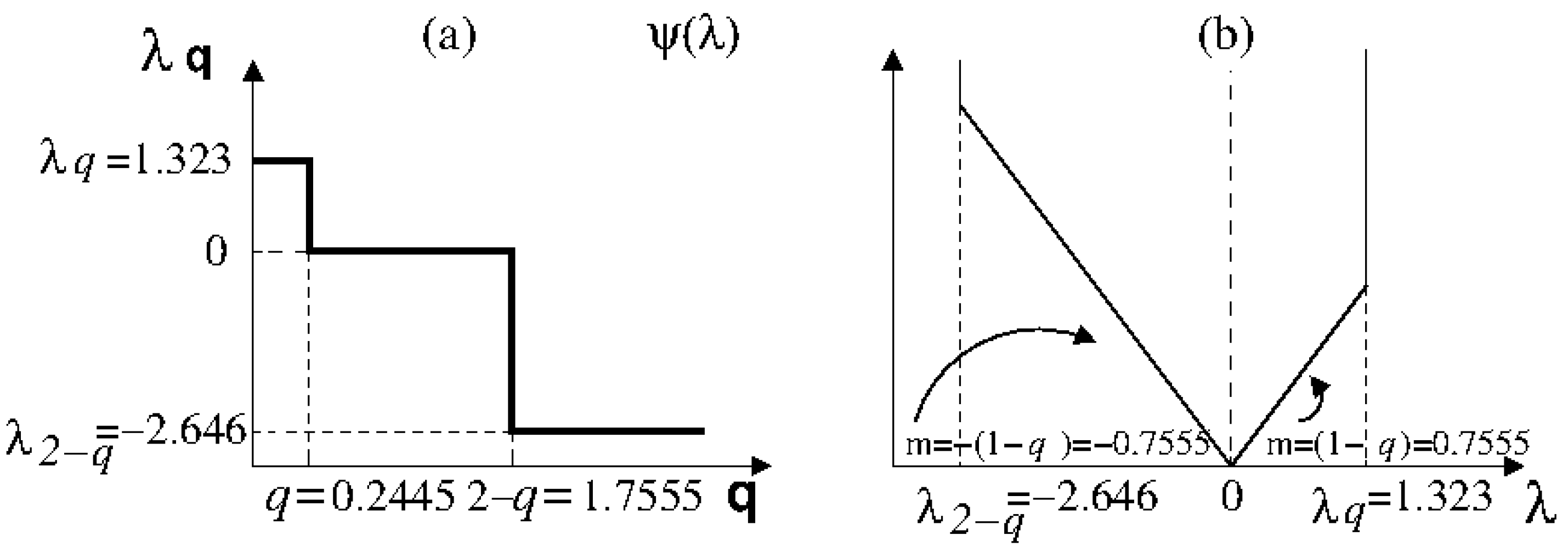
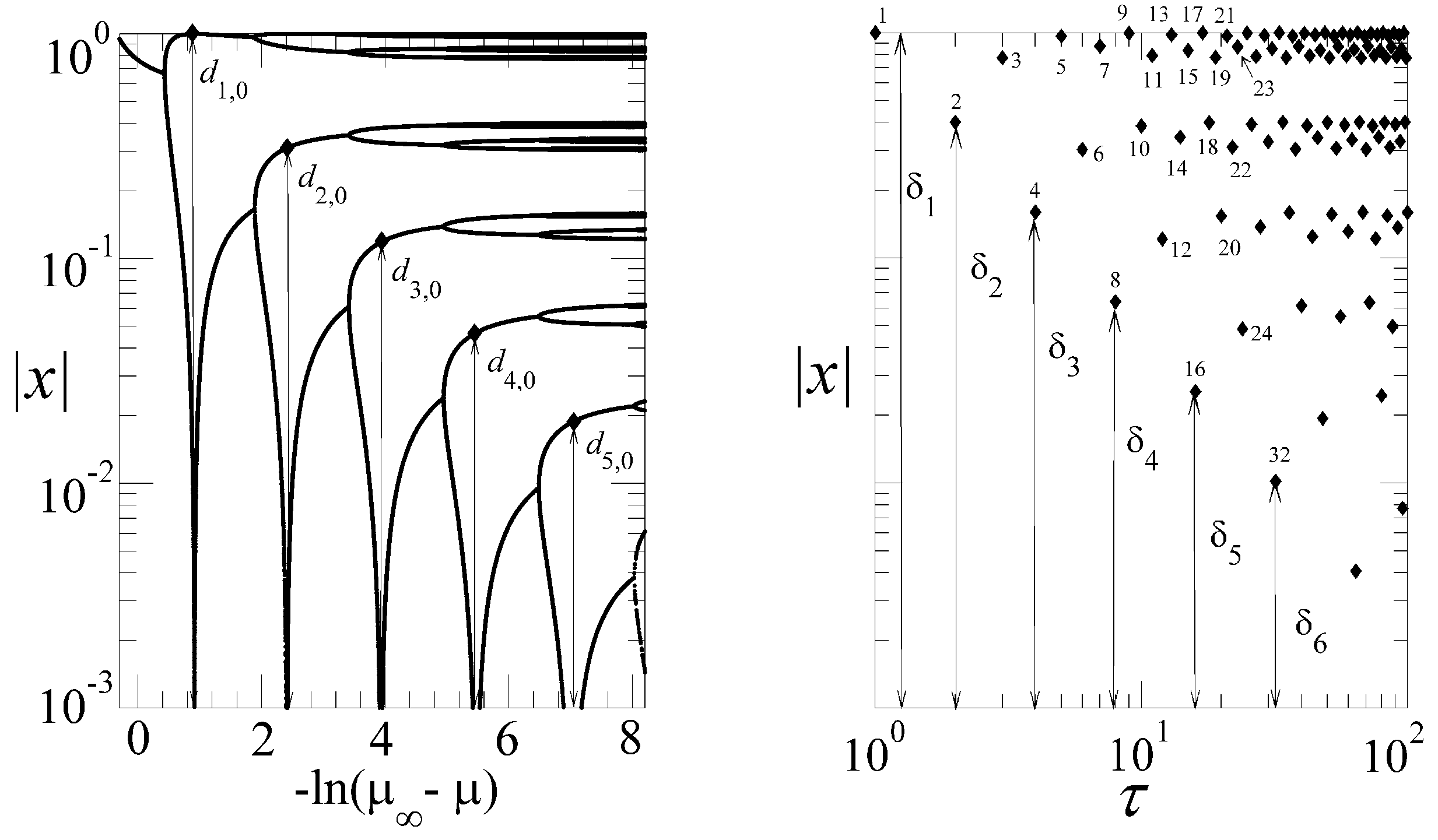
One of our most striking findings is that the dynamics at the period-doubling accumulation point is constituted by an infinite family of Mori’s q-phase transitions, each associated with orbits that have common starting and finishing positions located at specific regions of the multifractal attractor. Each of these transitions is related to a discontinuity in the trajectory scaling function, $\sigma (y)$, or “diameters ratio” function, and this, in turn, implies a q-exponential ${\xi }_t$ and a spectrum of q-Lyapunov coefficients for each set of orbits. The transitions come in pairs with specific conjugate indexes, q and $Q=2-q$, as these correspond to switching starting and finishing orbital positions. Since the amplitude of the discontinuities in σ diminishes rapidly, in practical terms, there is only the need for the evaluation for the first few of them. The dominant discontinuity is associated with the most crowded and sparse regions of the attractor, and this alone provides a very reasonable description. Thus, the special values for the Tsallis entropic index, q, in ${\xi }_t$ are equal to the special values of the variable $\mathsf{q}$ in the formalism of Mori and colleagues at which the q-phase transitions take place. We found that there is an infinite number of such special values, as there is an infinite number of universal discontinuities $\sigma (y)$. See [4] for a wider discussion.

Then, we recall that the approach of an ensemble of trajectories to the Feigenbaum attractor leads to a rich hierarchical structure with a generalized statistical-mechanical expression as an emergent property, an expression that contains an infinite number of q-indexes in the partition function linked to a thermodynamic potential also associated with a q-deformed exponential. Again, the values of all of these q-indexes are given in terms of the universal constants contained in the trajectory function, $\sigma (y)$. Both the trajectories within and those that approach the Feigenbaum attractor lead to stationary distributions for their sums of visited positions. As we have seen, these distributions capture the features of the dynamics associated with the multifractal attractor: the families of q-exponentials in the trajectory within the attractor (Figure 3), the formation of phase-space gaps (Figure 9), the hierarchical arrangements of the repellor positions and their preimages (Figure 11 and Figure 12).

In the case of the attractor-repellor fixed point that represents the tangent bifurcation, we have seen that there is a pure q-statistical regime, for the trajectories, $x_t$, the sensitivity, ${\xi }_t$, and the time extensivity of the entropy, $S_q$. A single q-index occurs (and naturally, also, its companion indexes, $2-q$ and $2-1/q$). This is reflected in the physical systems that accept a description analogous to this dynamics, the critical clusters, the conductance at the mobility edge and the rank distributions. However, as we have seen, the multifractal nature of the period-doubling accumulation point (and, similarly, the critical attractors of the quasiperiodic route to chaos in circle maps [6]) requires an infinite set of q-indexes and their duals, $2-q$, each, of course, given by the infinite set of universal constants contained in the trajectory scaling function, $\sigma (y)$. As described, there are infinite families of q-exponentials in the sensitivity within the attractor and in the configurational weights in the partition function. The anomalous dynamics within and towards this type of critical attractor cannot be described with a language simpler than that required to characterize the multifractal set itself. However, approximations can be introduced that reduce the infinite set of q-indexes to a basic pair, q and $2-q$. For the Feigenbaum attractor of the quadratic logistic map $\zeta =2$, the dominance of the two largest discontinuities in $\sigma (y)$, ${\alpha }^{-1}$ and ${\alpha }^{-2}$, which correspond, respectively, to the sparsest and tighter regions of the multifractal, suggests that a reasonable approximation is the consideration of only these two contributions, while the others are neglected. This approximation reduces the Feigenbaum attractor into a two-scale multifractal and a single index parameter $q=1-ln2/ln\alpha$ [5,39]. Furthermore, the time series transformation of the trajectories at the Feigenbaum attractor into a network via the HV algorithm reduces the multifractal nature in the dynamical properties into a single fractal description with only a single network generalized Lyapunov spectrum [25].

Since the early days of q-statistics, the presence of a duality in q-indexes and q-entropies have been noticed and documented. From a purely operational standpoint, their source is straightforward: the inverse of a q-exponential or, equivalently, the inverse of the argument of a q-logarithm, generates the dual indexes, q and $Q=2-q$. Differentiation of these functions give the twin indexes, q and $Q=1/q$, and a combination of both yields the pair $Q=2-1/q$. Larger sets of related q-indexes can be produced via iteration of these and other common algebraic and analytical procedures. Naturally, there appear dual physical quantities associated with them, e.g., generalized Lyapunov exponents and generalized Pesin identities. Their physical status and meanings can be answered by considering the results obtained for the different dynamical systems considered here. These point out that the view that between two possible entropy expressions, only one is to be a physical quantity, is inappropriate. We quote a statement from an earlier study [34]: “An interesting observation about the structure of the nonextensive formalism is that the equiprobability entropy expression ${ln}_q{W}_t$ can be obtained not only from $S_q$ in:

$$S_q\equiv \sum _i{p}_i{ln}_q\left(\frac{1}{p_i}\right)=\frac{1-{\sum }_i^W{p}_i^q}{q-1}$$

(52)

but also from

$$S_Q^{†}\equiv -\sum _{i=1}^W{p}_i{ln}_{{}_Q}{p}_i$$

(53)

where $S_Q^{†}=S_{2-Q}=S_q$. The inverse property of the q exponential reads ${ln}_q(y)=-{ln}_{2-q}(1/y)$ for the q logarithm and as pointed out introduces a pair of conjugate indices $Q=2-q$ with the consequence that, while some theoretical features are equally expressed by both $S_q$ and $S_Q^{†}$, some others appear only via the use of either $S_q$ or $S_Q^{†}$. For instance, the canonical ensemble maximization of $S_Q^{†}$ with the customary constraints ${\sum }_{i=1}^W{p}_i=1$ and ${\sum }_{i=1}^W{p}_i{\epsilon }_i=U$, where ${\epsilon }_i$ and U are configurational and average energies, respectively, leads to a Q-exponential weight (with $Q>1$ when $q<1$). On the other hand, the partition function is obtained via the optimization of $S_q$. The mutual Equations (52) and (53) elegantly generalize the BG entropy.”

Recently [55,56], the two entropy expressions in Equations (52) and (53) have been formally examined in relation to the maximum entropy principle (MEP) under the assumption that only the first three Shannon–Kinchin axioms hold. The dual entropies are known to follow from optimization involving different constraints: one is that quoted above, ${\sum }_{i=1}^W{p}_i{\epsilon }_i=U$; and the other is related to the modified “average” ${\sum }_{i=1}^W{p}_i^q{\epsilon }_i=U_q$. It is clear that the two constraints leading to the two entropy expressions play a role in the dynamics with a single pair of dual indexes, q and $2-q$, like in that associated with the tangent bifurcation and its manifestations in the description of critical clusters, mobility edge and rank distributions. However, for the case of a multifractal critical attractor, the MEP procedure calls for some generalization in order to accommodate the presence of an infinite set of q-indexes.

The common tenet in the studies reviewed here is that the properties of the systems considered are first determined independently of any method that assumes a statistical-mechanical formalism (other than the ordinary LGW Hamiltonian in the BG formalism for critical clusters in Subsection 5.1). That is, these properties are not derived under the supposition of the applicability of generalized entropy expressions or their implications. After that, the results obtained for these systems (trajectories, sensitivity, rates of approach, etc., and their counterparts in condensed matter and other interdisciplinarily complex systems) are analyzed in relation to generalized entropy expressions or properties derived from them. Finally, we commented on pertinent conclusions.

References

1. Beck, C.; Schlogl, F. Thermodynamics of Chaotic Systems; Cambridge University Press: Cambridge, UK, 1993. [Google Scholar]
2. Mori, H.; Rata, H.; Horita, T.; Kobayashi, T. Statistical mechanics of dynamical systems. Prog. Theor. Phys. Suppl. 1989, 99, 1–63. [Google Scholar] [CrossRef]
3. Baldovin, F.; Robledo, A. Sensitivity to initial conditions at bifurcations in one-dimensional nonlinear maps: Rigorous nonextensive solutions. Europhys. Lett. 2002, 60. [Google Scholar] [CrossRef]
4. Mayoral, E.; Robledo, A. Tsallis q index and Moris q phase transitions at the edge of chaos. Phys. Rev. E 2005, 72, 026209. [Google Scholar] [CrossRef] [PubMed]
5. Robledo, A.; Moyano, L.G. q-deformed statistical-mechanical property in the dynamics of trajectories en route to the Feigenbaum attractor. Phys. Rev. E 2008, 77, 036213. [Google Scholar] [CrossRef] [PubMed]
6. Hernández-Saldaña, H.; Robledo, A. Fluctuating dynamics at the quasiperiodic onset of chaos, Tsallis q-statistics and Mori’s q-phase thermodynamics. Physica A 2006, 370, 286–300. [Google Scholar] [CrossRef]
7. Baldovin, F. Routes to chaos, universality and glass formation. Physica A 2006, 372, 224–237. [Google Scholar] [CrossRef]
8. Schuster, H.G. Deterministic Chaos: An Introduction, 2nd ed.; VCH Publishers: Weinheim, Germany, 1988. [Google Scholar]
9. Hilborn, R.C. Chaos and Nonlinear Dynamics, 2nd ed.; Oxford University Press: New York, NY, USA, 2000. [Google Scholar]
10. Tsallis, C. Possible generalization of Boltzmann-Gibbs statistics. J. Stat. Phys. 1988, 52, 479–487. [Google Scholar] [CrossRef]
11. Tsallis, C. Introduction to Nonextensive Statistical Mechanics: Approaching a Complex World; Springer: New York, NY, USA, 2009. [Google Scholar]
12. Contoyiannis, Y.F.; Diakonos, F.K. Criticality and intermittency in the order parameter space. Phys. Lett. A 2000, 268, 286–292. [Google Scholar] [CrossRef]
13. Contoyiannis, Y.F.; Diakonos, F.K.; Malakis, A. Intermittent dynamics of critical fluctuations. Phys. Rev. Lett. 2002, 89, 035701. [Google Scholar] [CrossRef] [PubMed]
14. Robledo, A. Critical fluctuations, intermittent dynamics and Tsallis statistics. Physica A 2004, 344, 631–636. [Google Scholar] [CrossRef]
15. Robledo, A. Unorthodox properties of critical clusters. Mol. Phys. 2005, 103, 3025–3030. [Google Scholar] [CrossRef]
16. Martinez-Mares, M.; Robledo, A. Equivalence between the mobility edge of electronic transport on disorderless networks and the onset of chaos via intermittency in deterministic maps. Phys. Rev. E 2009, 80, 045201. [Google Scholar] [CrossRef] [PubMed]
17. Robledo, A. Universal glassy dynamics at noise-perturbed onset of chaos: A route to ergodicity breakdown. Phys. Lett. A 2004, 328, 467–472. [Google Scholar] [CrossRef]
18. Robledo, A. Aging at the edge of chaos: Glassy dynamics and nonextensive statistics. Physica A 2004, 342, 104–111. [Google Scholar] [CrossRef]
19. Baldovin, F.; Robledo, A. Parallels between the dynamics at the noise-perturbed onset of chaos in logistic maps and the dynamics of glass formation. Phys. Rev. E 2005, 72, 066213. [Google Scholar] [CrossRef] [PubMed]
20. Robledo, A. A dynamical model for hierarchy and modular organization: The trajectories en route to the attractor at the transition to chaos. J. Phys. Conf. Ser. 2012, 394, 012007. [Google Scholar] [CrossRef]
21. Fuentes, M.A.; Robledo, A. Renormalization group structure for sums of variables generated by incipiently chaotic maps. J. Stat. Mech. 2010, P01001. [Google Scholar] [CrossRef]
22. Fuentes, M.A.; Robledo, A. Stationary distributions of sums of marginally chaotic variables as renormalization group fixed points. J. Phys. Conf. Ser. 2012, 201, 012002. [Google Scholar] [CrossRef]
23. Fuentes, M.A.; Robledo, A. Sums of variables at the onset of chaos. Eur. Phys. J. B 2013. submitted for publication. [Google Scholar] [CrossRef]
24. Altamirano, C.; Robledo, A. Possible thermodynamic structure underlying the laws of Zipf and Benford. Eur. Phys. J. B 2011, 81, 345–351. [Google Scholar] [CrossRef]
25. Luque, B.; Lacasa, L.; Robledo, A. Feigenbaum graphs at the onset of chaos. Phys. Lett. A 2012, 376, 3625–3629. [Google Scholar] [CrossRef]
26. Ergodicity is referred here in relation to the total phase space on which the map is defined.
27. Baldovin, F.; Robledo, A. Universal renormalization-group dynamics at the onset of chaos in logistic maps and nonextensive statistical mechanics. Phys. Rev. E 2002, 66, 045104. [Google Scholar] [CrossRef] [PubMed]
28. Robledo, A. Incidence of nonextensive thermodynamics in temporal scaling at Feigenbaum points. Physica A 2006, 370, 449–460. [Google Scholar] [CrossRef]
29. Robledo, A. The renormalization group and optimization of non-extensive entropy: Criticality in non-linear one-dimensional maps. Physica A 2002, 314, 437–441. [Google Scholar] [CrossRef]
30. Robledo, A. Criticality in nonlinear one-dimensional maps: RG universal map and nonextensive entropy. Physica D 2004, 193, 153–160. [Google Scholar] [CrossRef]
31. Hu, B.; Rudnick, J. Exact solutions to the feigenbaum renormalization-group equations for intermittency. Phys. Rev. Lett. 1982, 48, 1645–1648. [Google Scholar] [CrossRef]
32. Barkai, E. Aging in subdiffusion generated by a deterministic dynamical system. Phys. Rev. Lett. 2003, 90, 104101. [Google Scholar] [CrossRef] [PubMed]
33. Gaspard, P.; Wang, X.J. Sporadicity: Between periodic and chaotic dynamical behaviors. Proc. Natl. Acad. Sci. USA 1988, 85, 4591–4595. [Google Scholar] [CrossRef] [PubMed]
34. Baldovin, F.; Robledo, A. Nonextensive Pesin identity: Exact renormalization group analytical results for the dynamics at the edge of chaos of the logistic map. Phys. Rev. E 2004, 69, 045202. [Google Scholar] [CrossRef] [PubMed]
35. Anania, G.; Politi, A. Dynamical behaviour at the onset of chaos. Europhys. Lett. 1988, 7. [Google Scholar] [CrossRef]
36. Hata, H.; Horita, T.; Mori, H. Dynamic description of the critical 2 attractor and 2m-band chaos. Progr. Theor. Phys. 1989, 82, 897–910. [Google Scholar] [CrossRef]
37. Moyano, L.G.; Silva, D.; Robledo, A. Labyrinthine pathways towards supercycle attractors in unimodal maps. Cent. Eur. J. Phys. 2009, 7, 591–600. [Google Scholar] [CrossRef]
38. Grassberger, P. Proposed central limit behavior in deterministic dynamical systems. Phys. Rev. E 2009, 79, 057201. [Google Scholar] [CrossRef] [PubMed]
39. Diaz-Ruelas, A.; Robledo, A. Emergent statistical-mechanical structure in the dynamics along the period-doubling route to chaos. Europhys. Lett. 2013. submitted for publication. [Google Scholar] [CrossRef]
40. Antoniou, N.G.; Contoyiannis, Y.F.; Diakonos, F.K.; Papadoupoulos, C.G. Fractals at T = Tc due to instantonlike configurations. Phys. Rev. Lett. 1998, 81, 4289–4292. [Google Scholar] [CrossRef]
41. Antoniou, N.G.; Contoyiannis, Y.F.; Diakonos, F.K. Fractal geometry of critical systems. Phys. Rev. E 2000, 62, 3125–3134. [Google Scholar] [CrossRef]
42. Crutchfield, J.P.; Farmer, J.D.; Huberman, B.A. Fluctuations and simple chaotic dynamics. Phys. Rep. 1982, 92, 45–82. [Google Scholar] [CrossRef]
43. For a review see: de Benedetti, P.G.; Stillinger, F.H. Supercooled liquids and the glass transition. Nature 2001, 410, 259–267. [Google Scholar]
44. De Benedetti, P.G. Metastable Liquids. Concepts and Principles; Princeton University Press: Princeton, NJ, USA, 1996. [Google Scholar]
45. Kaneko, K. Overview of coupled map lattices. Chaos 1992, 2, 279–282. [Google Scholar] [CrossRef] [PubMed]
46. See, for example: Chaikin, P.M.; Lubensky, T.C. Principles of Condensed Matter Physics; Cambridge University Press: Cambridge, UK, 1995. [Google Scholar]
47. Robledo, A. Laws of Zipf and Benford, intermittency, and critical fluctuations. Chin. Sci. Bull. 2011, 56, 3643–3648. [Google Scholar] [CrossRef]
48. Lacasa, L.; Luque, B.; Ballesteros, F.; Luque, J.; Nuño, J.C. From time series to complex networks: The visibility graph. Proc. Natl. Acad. Sci. USA 2008, 105, 4972–4975. [Google Scholar] [CrossRef] [PubMed]
49. Luque, B.; Lacasa, L.; Luque, J.; Ballesteros, F. Horizontal visibility graphs: Exact results for random time series. Phys. Rev. E 2009, 80, 046103. [Google Scholar] [CrossRef] [PubMed]
50. Luque, B.; Lacasa, L.; Ballesteros, F.; Robledo, A. Feigenbaum graphs: A complex network perspective of chaos. PLoS One 2011, 6. [Google Scholar] [CrossRef] [PubMed]
51. Luque, B.; Lacasa, L.; Ballesteros, F.; Robledo, A. Analytical properties of horizontal visibility graphs in the Feigenbaum scenario. Chaos 2012, 22, 013109. [Google Scholar] [CrossRef] [PubMed]
52. Luque, B.; Nuñez, A.; Ballesteros, F.; Robledo, A. Quasiperiodic graphs: Structural design, scaling and entropic properties. J. Nonlinear Sci. 2013, 23, 335–342. [Google Scholar] [CrossRef] [Green Version]
53. Núñez, A.M.; Luque, B.; Lacasa, L.; Gómez, J.P.; Robledo, A. Horizontal visibility graphs generated by type-I intermittency. Phys. Rev. E 2013, 87, 052801. [Google Scholar] [CrossRef] [PubMed]
54. Núñez, A.M.; Luque, B.; Cordero, M.; Gómez, M.; Robledo, A. Quasiperiodic graphs at the onset of chaos. Phys. Rev. E 2013. submitted for publication. [Google Scholar]
55. Hanel, R.; Thurner, S.; Gell-Mann, M. Generalized entropies and the transformation group of superstatistics. Proc. Natl. Acad. Sci. USA 2011, 108, 6390–6394. [Google Scholar] [CrossRef]
56. Hanel, R.; Thurner, S.; Gell-Mann, M. Generalized entropies and logarithms and their duality relations. Proc. Natl. Acad. Sci. USA 2012, 109, 19151–19154. [Google Scholar] [CrossRef] [PubMed]