Relaxation to Fixed Points in the Logistic and Cubic Maps: Analytical and Numerical Investigation

Abstract

Convergence to a period one fixed point is investigated for both logistic and cubic maps. For the logistic map the relaxation to the fixed point is considered near a transcritical bifurcation while for the cubic map it is near a pitchfork bifurcation. We confirmed that the convergence to the fixed point in both logistic and cubic maps for a region close to the fixed point goes exponentially fast to the fixed point and with a relaxation time described by a power law of exponent $-1$. At the bifurcation point, the exponent is not universal and depends on the type of the bifurcation as well as on the nonlinearity of the map.

1. Introduction

The motivation for studying discrete mappings comes in the last century from a seminal investigation by May [1], and since then a wide range of applications appeared involving different areas, including biology, physics, chemistry, mathematics, engineering and many others [2,3,4,5,6,7,8,9,10]. Comprehensive discussions on maps can also be found in [11,12,13,14,15,16].

In this paper, we revisit two well known maps namely the logistic map and the cubic map. The nonlinearity of the logistic map is quadratic while for the cubic map, and as the name suggests, is cubic. The two models experience a set of bifurcations reaching the chaos via period-doubling bifurcation and following normal Feingenbaum scaling [17,18]. Before reaching that, the logistic map experiences a transcritical bifurcation where an exchange of stability between fixed points happens and the cubic map experiences a pitchfork bifurcation with a fixed point losing stability, while a twin period one fixed point is born. Our main goal in this paper is to investigate the relaxation to the fixed point around these two bifurcations. We then use a set of numerical simulations and a theoretical investigation to show that, at the bifurcation, a convergence to the fixed point is given by a power law [19] with different exponents for the two bifurcation, while after the bifurcation, the convergence to the fixed point is exponential and with a relaxation time given by a power law with the same exponent for both bifurcations.

The paper is organized as follows. In Section 2 we discuss the mappings considered in this paper and the results obtained. Numerical simulations supporting theoretical findings are given in this Section too. Conclusions are drawn in Section 3.

2. The Mappings and Relaxation to the Fixed Points Investigation

We consider in this section the behavior of the relaxation to the fixed points for two mappings, namely the logistic map given by the expression

$$x_{n+1}=R_l{x}_n-R_l{x}_n^2$$

(1)

and for the cubic map given by

$$x_{n+1}=R_c{x}_n-x_n^3$$

(2)

where both $R_l$ and $R_c$ are control parameters. For our investigations in this paper we consider the ranges $R_l\in [0,4]$ and $R_c\in [0,3]$. For either $R_l>4$ and $R_c>3$ yields the dynamics to go to $-\infty$ and is without interest for us. Figure 1 shows the orbit diagram for the two mappings given by Equations (1) and (2).

As is well known in the literature, the logistic map has two fixed points for $R_l\in [0,3]$ namely

$$\begin{array}{ccc}\hfill x_1^l& =& 0\hfill \end{array}$$

(3)

$$\begin{array}{ccc}\hfill x_2^l& =& \frac{R_l-1}{R_l}\hfill \end{array}$$

(4)

where, according to stability analysis, $x_1^l$ is asymptotically stable for $R_l\in [0,1)$ while $x_2^l$ is asymptotically stable for $R_l\in (1,3)$ for any initial conditions lying $x_0\in (0,1)$. At $R_l=1$, the system experiences a transcritical bifurcation and fixed point $x_1^l$ changes stability with $x_2^l$. For $R_l=3$ the system exhibits a first period-doubling bifurcation following in a sequence of period-doubling until reaches chaotic behavior. At the bifurcations, the Lyapunov exponents are null given the eigenvalues at the bifurcation points are 1 or $-1$. The sequence of period-doubling follows a Feingenbaum scaling [17,18].

Figure 1. Bifurcation diagrams for: (a) logistic map and; (b) cubic map (for two different initial conditions). The names of some bifurcations are indicated in the figures.

For the cubic map, there is a fixed point $x_1^c=0$ and two period one fixed points $x_2^c=\sqrt{R_c-1}$ and $x_3^c=-\sqrt{R_c-1}$ both are born at $R_c=1$. At $R_c=1$ the system experiences a pitchfork bifurcation when $x_1^c$ loses stability and there is a birth of the $x_{2,3}^c$ fixed points. Each one of them evolve independently suffering period-doubling bifurcations until reach the chaos. Again the sequences of period-doubling are described by the Feingenbaum scaling [17,18]. The two separate chaotic bands are merged only due to a merging chaotic attractors crisis [13,14].

The two regions we are interested in to discuss along this paper correspond to: (i) the region of the transcritical bifurcation in the logistic map and; (ii) the region of the pitchfork bifurcation in the cubic map. Indeed we are seeking to understand and describe how is the relaxation of orbits starting close to the fixed point near both bifurcations. We are then looking to describe the behavior of x approaching to $x^{*}$ denoting the fixed points at $R_l=1$ and $R_c=1$. Exactly like any other variable, x is a function of two entities, i.e., n which is the number of iterations and $\mu =R_l-1$ for the logistic map and $\mu =R_c-1$ for cubic for both $R_{l,c}\ge 1$.

Following previous results in the literature [19,20], we start with two hypotheses:

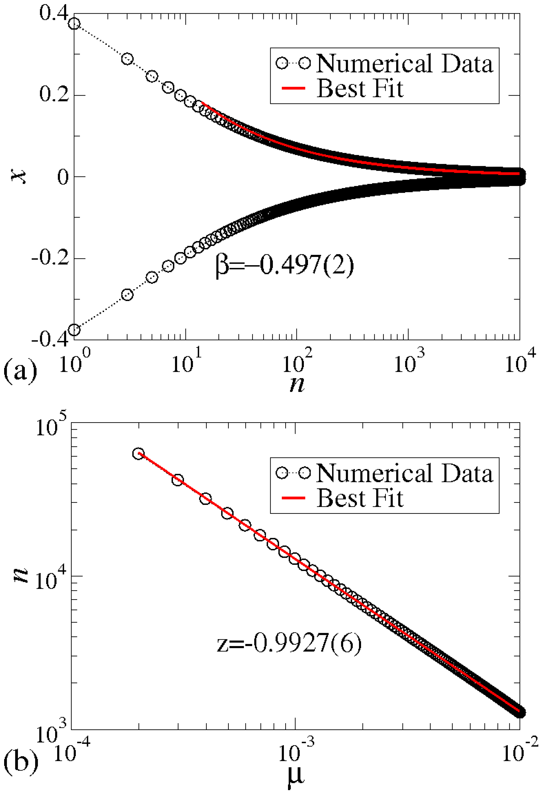
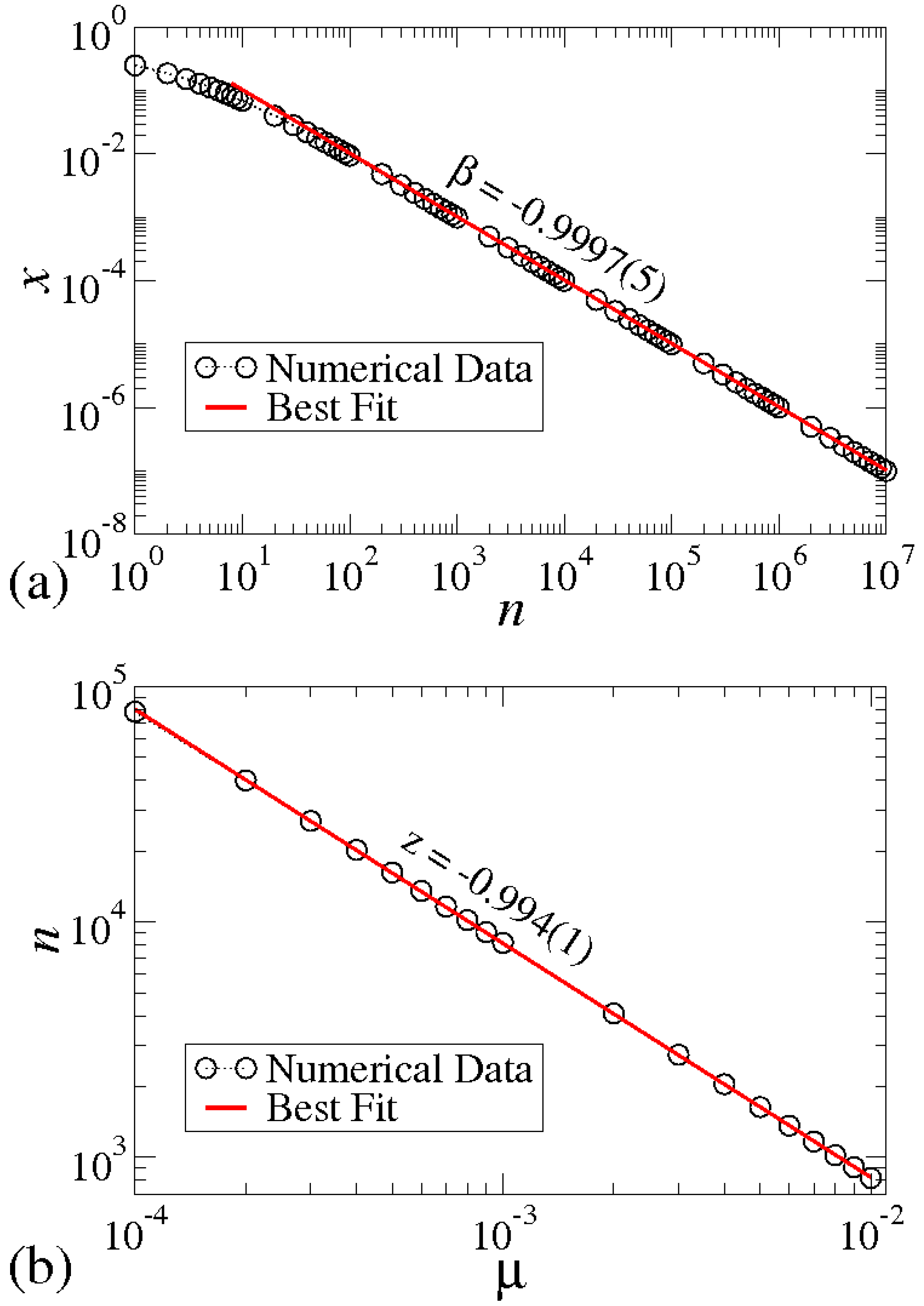
• For $\mu =0$ it implies there is an algebraic decay in x so that

  $$x(n,\mu =0)\propto n^{\beta }$$

  (5)

  where β is a critical exponent and depends on the type of bifurcation.
• For the parameter $\mu \ne 0$, we assume the orbit relaxes to the equilibrium exponentially according to

  $$x(n,\mu )\propto e^{-\frac{n}{\tau }}$$

  (6)

  where the relaxation time τ has the following form

  $$\tau \propto {\mu }^z$$

  (7)

  where z is also a critical exponent.

Before showing some theoretical approaches to describe the critical exponents, let us first check what a numerical simulation provides. Figure 2 shows a plot of the convergence to the fixed point considering the logistic map for: (a) $\mu =0$ and (b) $\mu \ne 0$.

Figure 2. Convergence to the fixed point for the logistic map considering: (a) $\mu =0$ where a power law fit furnishes $\beta =-0.99997\left(5\right)\cong -1$ and; (b) $\mu \ne 0$ with a slope of $z=-0.994\left(1\right)\cong -1$.

After doing power law fittings for the two plots of Figure 2 we obtain that $\beta =-0.99997\left(5\right)\cong -1$ and $z=-0.994\left(1\right)\cong -1$.

On the other hand the convergence to the fixed point for the cubic map is shown in Figure 3 for: (a) $\mu =0$ leading to a slope of decay given by $\beta =-0.497\left(2\right)\cong -1/2$ and; (b) $\mu \ne 0$ yielding in a slope of $z=-0.9927\left(6\right)\cong -1$.

Figure 3. Convergence to the fixed point for the cubic map considering: (a) $\mu =0$ where a power law fit furnishes $\beta =-0.497\left(2\right)\cong -1/2$ and; (b) $\mu \ne 0$ with a slope of $z=-0.9927\left(6\right)\cong -1$.

Given the numerical results are now known, we can go ahead with the theoretical argumentation on the characterization of the relaxations. Let us start with the logistic map as example and considering the transcritical bifurcation, i.e., $R_l=1$. In this case the mapping is written as

$$x_{n+1}=x_n-x_n^2$$

(8)

Equation (8) can be rewritten in a more convenient way as

$$x_{n+1}-x_n=\frac{x_{n+1}-x_n}{(n+1)-n}\cong \frac{dx}{dn}$$

(9)

that leads to the following approximation

$$\frac{dx}{dn}=-x^2$$

(10)

The approach used in Equation (10) is only valid in the limit of $x\left(n\right)$ very close to the fixed point. In such a limit, the discrete variables can be treated like a continuous variable, making the derivative possible.

Integrating Equation (10) from both sides leads to

$${\int }_{x_0}^x\frac{1}{{x^{\prime }}^2}d{x}^{\prime }={\int }_0^{n}d{n}^{\prime }$$

(11)

After doing the integration and rearranging the terms properly we end up with

$$x\left(n\right)=\frac{1}{n+\frac{1}{x_0}}$$

(12)

As soon as n grows attending to the condition $n\gg 1/x_0$ we obtain

$$x\left(n\right)\propto n^{-1}$$

(13)

After a comparison with Equation (5) we see that for the logistic map at $R_l=1$ the critical exponent $\beta =-1$, in well agreement to the numerical results presented in Figure 2.

The investigation for $R_l>1$ is quite similar to the previous case with a minimal detail of subtracting from both sides of Equation (1) a term $x_n$, that leads to

$$x_{n+1}-x_n=\frac{x_{n+1}-x_n}{(n+1)-n}\cong \frac{dx}{dn}$$

(14)

yielding at the end with an expression of the type

$$\frac{dx}{dn}=x(R_l-1)-R_l{x}^2$$

(15)

When x is sufficiently close to the fixed point, the second term of Equation (15) which is a quadratic term, becomes rather small as compared to the first one becoming then negligible. Because of this it indeed can be disregarded. Quoting the definition of μ we can rewrite Equation (15) as

$$\frac{dx}{dn}=x\mu$$

(16)

which in terms of integral is given as

$${\int }_{x_0}^x\frac{d{x}^{\prime }}{x^{\prime }}=\mu {\int }_0^{n}d{n}^{\prime }$$

(17)

Doing the integral properly we obtain that

$$x\left(n\right)=x_0{e}^{\mu n}$$

(18)

A comparison with Equation (6) leads us to conclude that the critical exponent $z=-1$, again is in well agreement with the simulation, as confirmed in Figure 2.

Let us now continue the investigation but considering this time the cubic map for $R_c=1$. Doing similar procedure as made in Equation (9) we obtain

$$\frac{dx}{dn}=-x^3$$

(19)

After doing the integration and organize the terms properly we obtain that

$$\begin{array}{ccc}\hfill x\left(n\right)& =& \sqrt{\frac{1}{2n+\frac{1}{x_0^2}}}\hfill \\ & \cong & \frac{1}{\sqrt{2}}{n}^{-\frac{1}{2}}\hfill \end{array}$$

(20)

for the limit of $2n\gg 1/x_0^2$. Comparing the result obtained from Equation (20) with the one presented in Equation (5) we find $\beta =-1/2$ which is confirmed by the numerical simulations shown in Figure 3.

Considering the case of $R_c>1$ but still close to 1, we end up with an expression of the type

$$\frac{dx}{dn}=x\mu -x^3$$

(21)

Using similar arguments as used for the logistic map, the cubic term in Equation (21) can be disregarded leading to an identical expression as given by Equation (18). Therefore we conclude that the critical exponent is given by $z=-1$ as indeed confirmed by numerical simulations presented in Figure 3.

The two mappings present a bifurcation in $R_{l,c}=1$. At the bifurcation point, both maps exhibit algebraic relaxation to the fixed point but with different critical exponents. For the logistic map $\beta =-1$ while for the cubic map it is given by $\beta =-1/2$. On the other hand, after the bifurcation takes place, the relaxation for the fixed point is given by the same law and with the same critical exponent $z=-1$.

Let us now discuss shortly on the behavior of the entropy for the bifurcations observed at $R_{l,c}=1$. To define a K-entropy, we follow same general discussion as made in [21]. The procedure starts from the evolution in time of a single initial condition converging towards an attractor. The region defining the attractor is therefore covered by a set of discrete cells. An initial condition is started along such cells and its trajectory is followed and marked in the phase space saying what cell is visit at stage n, as for example $x\left(0\right)\to x\left(1\right)\to x\left(2\right)\to x\left(3\right)\dots$. A second initial condition is started very close to the first one and that may lead to a different sequence of visits. The process continue to a very large number of initial conditions such that an ensemble average on the initial conditions can be made. From the average, a relative number of times a specific sequence of N cells is visited can be defined. Then the entropy $S_N$ is given as

$$S_N=<\sum _{i}p\left(i\right)ln\left(p\left(i\right)\right)>$$

(22)

where $p\left(i\right)$ gives the relative number for the ith sequence and with the summation taken over all possible sequences starting with $x\left(0\right)$. From this, the K-entropy is then defined as

$$K=\underset{N\to \infty }{lim}\frac{1}{N}(S_n-S_0)$$

(23)

Because the convergence to the attractor at $R_{l,c}=1$ is indeed an evolution towards an attracting fixed point, the dynamics is regular. Therefore all sequences starting from the same sufficiently small cell are the same, all orbits follow each other as time passes. This leads to $S_N=0$ for all the ensemble of N. For a large enough N produces a $K=0$ because there is no change in S. This is only observed because the dynamics is regular and no chaos is present for $R_{l,c}=1$.

3. Conclusions

We have considered in this paper the convergence to the fixed point by using two different mappings with different nonlinearities, namely the logistic map with a quadratic nonlinearity and the cubic map, whose nonlinearity is cubic. Both mappings are characterized by a control parameter that induces bifurcations in the system. For the logistic, the convergence to the fixed point at a transcritical bifurcation is given by a power law with exponent $\beta =-1$. In the cubic map at a pitchfork bifurcation, the decay to the fixed point is also algebraic with slope $\beta =-1/2$. After bifurcation the two systems show an exponential decay to the fixed point whose relaxation time is given by a power law with the same exponent for both maps, namely $z=-1$.

References

- May, R.M. Biological populations with non overlapping generations: Stable points, a stable cycles and chaos. Science 1974, 86, 645–647. [Google Scholar] [CrossRef]
- Hamacher, K. Dynamical regimes due to technological change in a microeconomical model of production. Chaos 2012, 22, 033149. [Google Scholar] [CrossRef] [PubMed]
- McCartney, M. Lyapunov exponents for multi-parameter tent and logistic maps. Chaos 2012, 21, 043104. [Google Scholar] [CrossRef] [PubMed]
- Philominathan, P.; Santhiah, M.; Mohamed, I.R.; Murali, K.; Rajasekar, S. Chaotic dynamics of a simple parametrically driven dissipative circuit. Int. J. Bifurc. Chaos 2011, 21, 1927–1933. [Google Scholar] [CrossRef]
- Santhiah, M.; Philominathan, P. Statistical dynamics of parametrically perturbed sine-square map. Pramana J. Phys. 2010, 75, 403–414. [Google Scholar] [CrossRef]
- Zhang, Y.-G.; Zhang, J.-F.; Ma, Q.; Ma, J.; Wang, Z.-P. Statistical description and forecasting analysis of life system. Int. J. Nonlinear Sci. Numer. Simul. 2010, 11, 157–164. [Google Scholar] [CrossRef]
- Hu, W.; Zhao, G.-H.; Zhang, G.; Zhang, J.-Q.; Liu, X.-L. Stabilities and bifurcations of sine dynamic equations on time scale. Acta Phys. Sin. 2012, 17, 170505. [Google Scholar]
- Urquizu, M.; Correig, A.M. Fast relaxation transients in a kicked damped oscillator. Chaos, Solitons Fractals 2007, 33, 1292–1306. [Google Scholar] [CrossRef]
- Livadiotis, G. Numerical approximation of the percentage of order for one-dimensional maps. Adv. Complex Syst. 2005, 8, 15–32. [Google Scholar] [CrossRef]
- Ilhem, D.; Amel, K. One-dimensional and two-dimensional dynamics of cubic maps. Discret. Dyn. Nat. Soc. 2006, 2006, 15840. [Google Scholar] [CrossRef]
- Li, T.Y.; Yorke, J.A. Period three implies chaos. Am. Math. Mon. 1975, 82, 985–992. [Google Scholar] [CrossRef]
- May, R.M.; Oster, G.A. Bifurcation and dynamical systems in simple ecological models. Am. Nat. 1976, 110, 573–599. [Google Scholar] [CrossRef]
- Grebogi, C.; Ott, E.; Yorke, J.A. Chaotic attractors in crisis. Phys. Rev. Lett. 1982, 48, 1507–1510. [Google Scholar] [CrossRef]
- Grebogi, C.; Ott, E.; Yorke, J.A. Crises, sudden changes in chaotic attractors, and transient chaos. Physica D 1983, 7, 181–200. [Google Scholar] [CrossRef]
- Gallas, J.A.C. Structure of the parameter space of the Hénon map. Phys. Rev. Lett. 1983, 70, 2714–2717. [Google Scholar] [CrossRef] [PubMed]
- Collet, P.; Eckmann, J.-P. Iterated Maps on the Interval as Dynamical Systems; Birkhauser: Boston, MA, UA, 1980. [Google Scholar]
- Feigenbaum, M.J. Universal metric properties of non-linear transformations. J. of Stat. Phys. 1979, 21, 669–706. [Google Scholar] [CrossRef]
- Feigenbaum, M.J. Quantitative universality for a class of non-linear transformations. J. Stat. Phys. 1978, 19, 25–52. [Google Scholar] [CrossRef]
- Leonel, E.D.; da Silva, J.K.L.; Kamphorst, S.O. Relaxation and transients in a time-dependent logistic map. Int. J. Bifurc. Chaos 2002, 12, 1667–1674. [Google Scholar] [CrossRef]
- Hohenberg, P.C.; Halperin, B.I. Theory of dynamic critical phenomena. Rev. Mod. Phys. 1977, 49, 435–479. [Google Scholar] [CrossRef]
- Hilborn, R.C. Chaos and Nonlinear Dynamics: An Introduction for Scientists and Engineers; Oxford University Press: New York, NY, USA, 1994. [Google Scholar]
© 2013 by the authors; licensee MDPI, Basel, Switzerland. This article is an open access article distributed under the terms and conditions of the Creative Commons Attribution license (http://creativecommons.org/licenses/by/3.0/).