An Entropic Estimator for Linear Inverse Problems

Abstract
:1. Introduction
 and
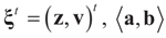
and 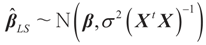 where “t” stands for transpose.
 2. Problem Statement and Solution
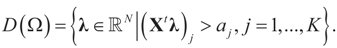
2.1. Notation and Problem Statement
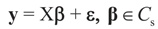
 is an unknown K-dimensional signal vector that cannot be directly measured but is required to satisfy some convex constraints expressed as
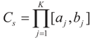
  where Cs is a closed convex set. For example,
  with constants
  . (These constraints may come from constraints on
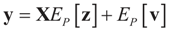
  , and may have a natural reason for being imposed). X is an N × K known linear operator (design matrix) that can be either fixed or stochastic,
  is a vector of noisy observations, and
  is a noise vector. Throughout this paper we assume that the components of the noise vector ε are i.i.d. random variables with zero mean and a variance σ2 with respect to a probability law dQn(v) on
  We denote by Qs and Qn the prior probability measures reflecting our knowledge about β and ε respectively.
  and the residuals
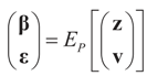
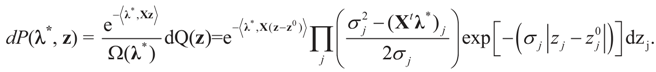
  so that Equation (1) holds. For that, we convert problem (1) into a generalized moment problem and consider the estimated β and ε as expected values of random variables z and v with respect to an unknown probability law P. Note that z is an auxiliary random variable whereas v is the actual model for the noise perturbing the measurements. Formally:. Further, in some cases the researcher may know the statistical model of the noise. In that case, this model should be used. As stated earlier, Qs and Qn are the prior probability measures for β and ε respectively. To ensure that the expected values of z and v fall in C = Cs × Cn we need the following assumption.
2.2. The Solution

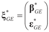
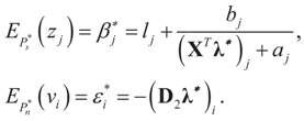
 is a random estimator of the unknown parameter vector β and
  is an estimator of the noise.
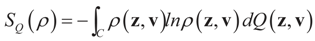
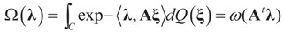
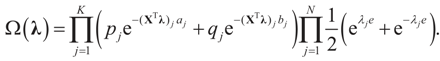
 denotes the Euclidean scalar (inner) product of vectors a and b, and
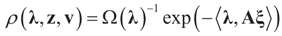
  are N free parameters that will play the role of Lagrange multipliers (one multiplier for each observation). The quantity Ω(λ) is the normalization function:

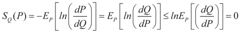
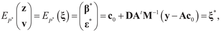
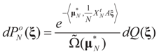
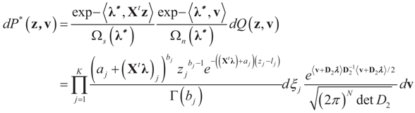
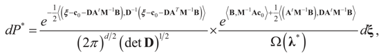
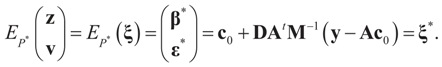
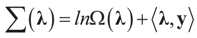 and for any ρ in the class of probability laws P(C) defined in (5). However, the problem is that we do not know whether the solution ρ*(λ, z, v) is a member of P(C) for some λ. Therefore, we search for λ* such that ρ* = ρ(λ*) is in P(C) and λ* is a minimum. If such a λ* is found, then we would have found a density (the unique one, for SQ is strictly convex in ρ) that maximizes the entropy, and by using the fact that β* = EP* [z] and ε* = EP* [v], the solution to (1), which is consistent with the data (3), is found. Formally, the result is contained in the following theorem. (Note that the Kullback’s measure (Kullback [34]), is a particular case of SQ(P), with a sign change and when both P and Q have densities).
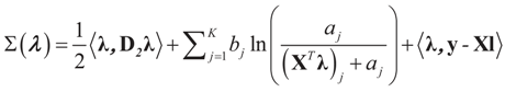
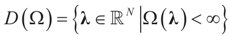 has a non-empty interior and that the minimum of the (convex) function ∑(λ) is achieved at λ*. Then,
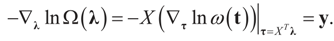
  satisfies the set of constrains (3) or (1) and maximizes the entropy.
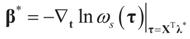
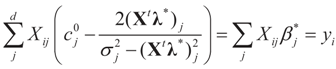
 which coincides with Equation (3) when the gradient is written out explicitly.
 is automatically satisfied. Since the actual measurement noise is unknown, it is treated as a quantity to be determined, and treated (mathematically) as if both β and ε were unknown. The interpretations of the reconstructed residual ε* and the reconstructed β*, are different. The latter is the unknown parameter vector we are after while the former is the residual (reconstructed error) such that the linear Equation (1),
  , is satisfied. With that background, we now discuss the basic properties of our model. For a detailed comparison of a large number of IT estimation methods see Golan ([27,28,29,30,31,32,33]) and the nice text of Mittelhammer, Judge and Miller [36]
 3. Closed Form Examples
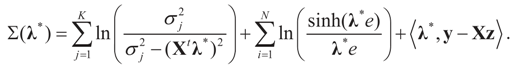
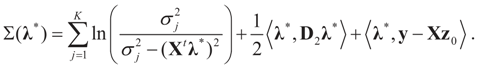
3.1. Normal Priors
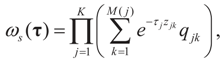
 where
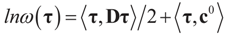
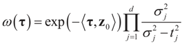
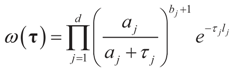
where  is the vector of prior means and is specified by the researcher. Next, we define the Laplace transform, ω(τ), of the normal prior. This transform involves the diagonal covariance matrix for the noise and signal models:

 then replacing τ by either Xtλ or by λ, (for the noise vector) verifies that Ω(λ) turns out to be of a quadratic form, and therefore the problem of minimizing ∑(λ) is just a quadratic minimization problem. In this case, no bounds are specified on the parameters. Instead, normal priors are used.
 and therefore:
 . See Appendix 2 for a detailed derivation.
3.2. Discrete Uniform Priors — A GME Model
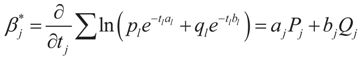
 for 1 ≤ k ≤ K Note that we allow for the cardinality of each of these sets to vary. Next, define
  . A similar construction may be proposed for the noise terms, namely we put
  . Since the spaces are discrete, the information is described by the obvious σ-algebras and both the prior and post-data measures will be discrete. As a prior on the signal space, we may consider:


 and
and  . For detailed derivations and discussion of the GME see Golan, Judge and Miller [1].
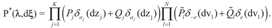
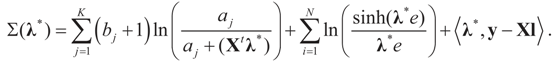
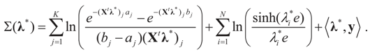
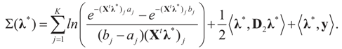
 3.3. Signal and Noise Bounded Above and Below
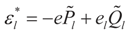
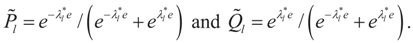
 and
and 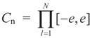 for the signal and noise bounds aj, bj and e respectively. The Bernoulli a priori measure on C = Cs × Cn is:


 and
and 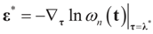 . Explicitly:

4. Main Results
4.1. Large Sample Properties
4.1.1. Notations and First Order Approximation
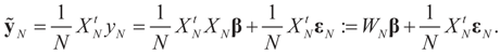
 the estimator of the true β when the sample size is N. Throughout this section we add a subscript N to all quantities introduced in Section 2 to remind us that the size of the data set is N. We want to show that
  and
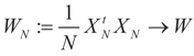
and 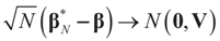 as N → ∞ in some appropriate way (for some covariance V). We state here the basic notations, assumptions and results and leave the details to the Appendix. The problem is that when N varies, we are dealing with problems of different sizes (recall λ is of dimension N in our generic model). To turn all problems to the same size let:
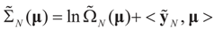
 .and
.and 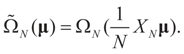
 More precisely, assume that
 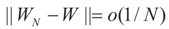 as N → ∞. Assume as well that for any N-vector v, as
 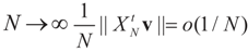 .
.  converge to 0 in L2, therefore in probability. To see the logic for that statement, recall that the vector εN has covariance matrix σ2IN. Therefore,
 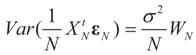 and assumption 4.1 yields the above conclusion. (To keep notations simple, and without loss of generality, we discuss here the case of σ2IN.)
 . Let
. Let  where β is the true but unknown vector of parameters. Then,
 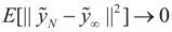 as N → ∞ (the proof is immediate).
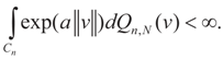 Then, for ,
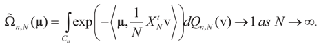
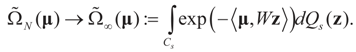
 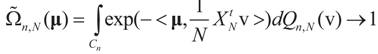 as N → ∞. Equivalently,
 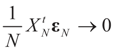 as N → ∞ weakly in
  with respect to the appropriate induced measure.:
 Then, under Assumption 4.1:
 satisfies:
 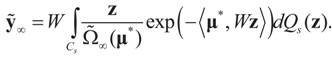 Or since W is invertible, β admits the representation
 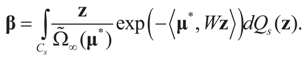 Note that this last identity can be written as
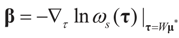
 To relate the solution to problem (1) to that of problem (15), observe that
  as well as
  where ΩN and ∑N are the functions introduced in Section 2 for a problem of size N. To relate the solution of the problem of size K to that of the problem of size N, we have:
 denotes the minimizer of
  then
then 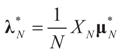 is the minimizer of ∑N(λ).
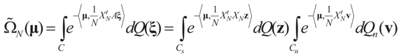
 is the solution for the N-dimensional (data) problem and
  is the solution for the moment problem, we have the following result:
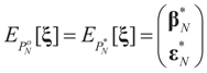 .
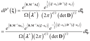
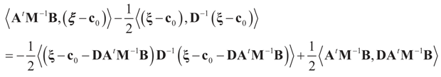
. defined by:

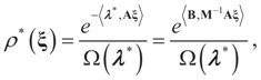
 the measure with density
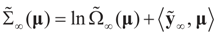
  with respect to Q. The invertibility of the functions defined above is related to the non-singularity of their Jacobian matrices, which are the -covariances of ξ. These functions will be invertible as long as these quantities are positive definite. The relationship among the above quantities is expressed in the following lemma:
 and
and  where
where  ,
,  and θ' is the first derivative of θ.
 are uniformly (with respect to N and μ) bounded below away from zero.
 4.1.2. First Order Unbiasedness
 as N →∞. Then up to o(1/N), is an unbiased estimator of β.
4.1.3. Consistency
 .
. in square mean as N → ∞.
- (a)
![Entropy 14 00892 i114]() as N → ∞,
as N → ∞,- (b)
![Entropy 14 00892 i115]() as N → ∞,
as N → ∞,


 stands for convergence in distribution (or law).
4.2. Forecasting
 . For example, if vf is centered (on 0), then
  and:
and:

5. Method Comparison
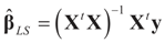
5.1. The Least Squares Methods
5.1.1. The General Case
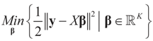
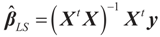
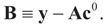
 may fall outside the range
  of X, so the objective is to minimize that discrepancy. The minimizer
  of (16) provides us with the LS estimates that minimize the errors sum of square distance from the data to
  . When (XtX)− exists, then
  . The reconstruction error
  can be thought of as our estimate of the “minimal error in quadratic norm” of the measurement errors, or of the noise present in the measurements.
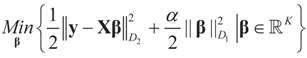
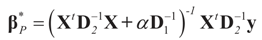
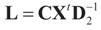
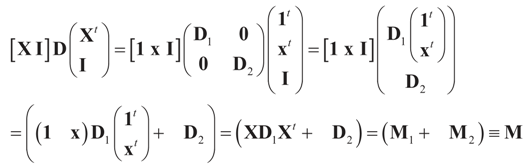
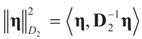 . In this case we get the GLS solution
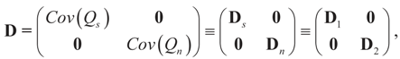
 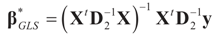 for any general (covariance) matrix D with blocks D1 and D2.
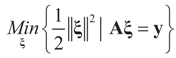
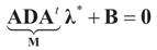
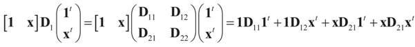
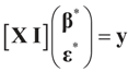
 ,
,  and the matrix A is of dimension N × (N + K), there are infinitely many solutions that satisfy the observed data in (1) (or (17)). To choose a single solution we solve the following model:
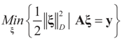
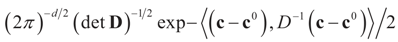
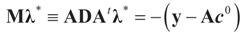
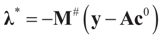
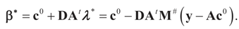
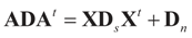
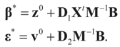
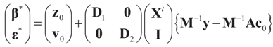
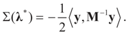
 is a weighted norm in the extended signal-noise space (C = Cs × Cn) and D can be taken to be the full covariance matrix composed of both D1 and D2 defined in Section 3.1. Under the assumption that M ≡ (ADAt) is invertible, the solution to the variational problem (19) is given by
  . This solution coincides with our Generalized Entropy formulation when normal priors are imposed and are centered about zero (c0 = 0) as is developed explicitly in Equation (14).
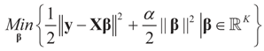
 , we can state the following.
 for α = 1. amounts to:

 with
with  is stated below. = when the constraints are in terms of pure moments (zero moments). = , then
 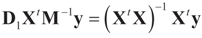 for all y, which implies the following chain of identities:
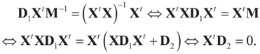
5.1.2. The Moments’ Case
= is the trivial condition XtD2X = 0.
5.2. The Basic Bayesian Method
 and respectively and that
  and
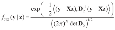
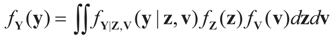
and  . For the rest of this section, the priors gn(v) will have their usual Bayesian interpretation. For a given z, we think of y = Xz + v as a realization of the random variable Y = Xz + V. Then,
 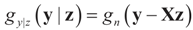 . The joint density gy,z(y,z) of Y and Z, where Z is distributed according to the prior Qs is:

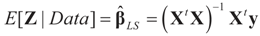
 and therefore by Bayes Theorem the posterior (post-data) conditional
  is
is  from which:
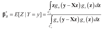
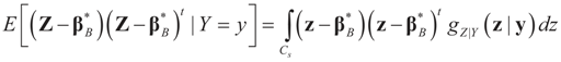
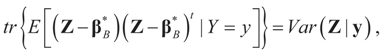
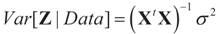
 minimizes
 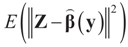 where Z and Y are distributed according to gy,z (y,z). The conditional covariance matrix:
5.2.1. A Standard Example: Normal Priors
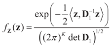
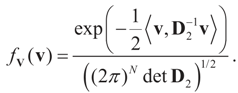
 . The conditional distribution of Z given Y is easy to obtain under the normal setup. Thus, the post-data distribution of the signal, β, given the data y is:
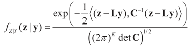
 and
and 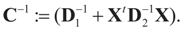 That is, “the posterior (post-data)” distribution of Z has changed (relative to the prior) by the data. Finally, the post-data expected value of Z is given by:
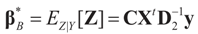
 , which is contained in D2. In the Bayesian result is marginalized, so it is not conditional on that parameter. Therefore, with a known value of , both estimators are the same.
 5.3. Comparison with the Bayesian Method of Moments (BMOM)
 which is assumed to be the post data mean with respect to (yet) unknown distribution (likelihood). This is equivalent to assuming
  (the columns of X are orthogonal to the N × 1 vector E[V|Data]). To find g(z|Data), or in Zellener’s notation g(β|Data), one applies the classical ME with the following constraints (information):
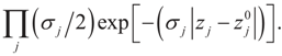
 is based on the assumption that
 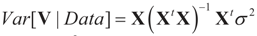 , or similarly under Zellner’s notation
 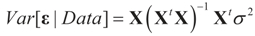 , and σ2 is a positive parameter. Then, the maximum entropy density satisfying these two constraints (and the requirement that it is a proper density) is:
 under the two side conditions used here. If more side conditions are used, the density function g will not be normal. Information other than moments can also be incorporated within the BMOM. of the unconstrained problem (1). Under the GE model, the solution satisfies the data/constraints within the joint support space C. Further, for the GE construction there is no need to impose exact moment constraints, meaning it provides a more flexible post data density. Finally, under both methods one can use the post data densities to calculate the uncertainties around future (unobserved) observations.
 6. More Closed Form Examples
6.1. The Basic Formulation
 The parameters
  is the set of prior means and 1/2σj is the variance of each component. The Laplace transform of dQ is:
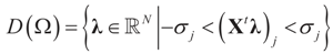 where ω(t) is always finite and positive. For this relationship to be satisfied,
  for all j = 1, 2, …, d. Finally, replacing τ by Xtλ yields D(Ω).
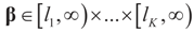
 , where [lj,∞) = [Zj,∞). Like related methods, we assume that each component Zj of Z is distributed in [lj,∞) according to a translated
  . With this in mind, a direct calculation yields:
6.1.2. Uniform Reference Measure
 and the Laplace transform of this density is:
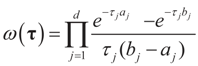
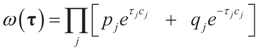
6.1.3. Bernoulli Reference Measure
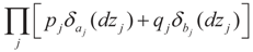 , where δc(dz) denotes the (Dirac) unit point mass at some point c, and where pj and qj do not have to sum up to one, yet they determine the weight within the bounded interval [aj, bj]. The Laplace transform of dQ is:

 yields estimates that are very similar to the continuous uniform prior.
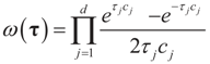
6.2 The Full Model
6.2.1. Bounded Parameters and Normally Distributed Errors
 but we impose no constraints on the ε. From Section 2,
 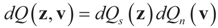 with
with 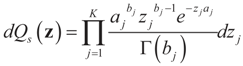 , and
, and 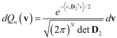 . The signal component is formulated earlier, while
 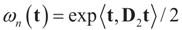 . Using A=[X I] we have
 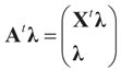 for the N-dimensional vector λ, and therefore,
 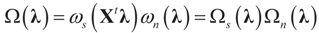 . The maximal entropy probability measures (post-data) are:
 and l determines the “shift” for each coordinate. (For example, if
  , then
 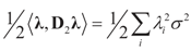 , or for the simple heteroscedastic case, we have ). Finally, once λ* is found, we get:
 , then , or for the simple heteroscedastic case, we have .
7. A Comment on Model Comparison

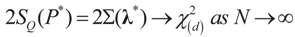 where d is the dimension of λ. This is the entropy ratio statistics which is similar in nature to the empirical likelihood ratio statistic (e.g., Golan [27]). Rather than discussing this statistic here, we provide in Appendix 3 analytic formulations of Equation (39) for a large number of prior distributions. These formulations are based on the examples of earlier sections. Last, we note that in some cases, where the competing models are of different dimensions, a normalization of both statistics is necessary.
8. Conclusions
Acknowledgments
References
- Golan, A.; Judge, G.G.; Miller, D. Maximum Entropy Econometrics: Robust Estimation with Limited Data; John Wiley & Sons: New York, NY, USA, 1996. [Google Scholar]
- Gzyl, H.; Velásquez, Y. Linear Inverse Problems: The Maximum Entropy Connection; World Scientific Publishers: Singapore, 2011. [Google Scholar]
- Jaynes, E.T. Information theory and statistical mechanics. Phys. Rev. 1957, 106, 620–630. [Google Scholar] [CrossRef]
- Jaynes, E.T. Information theory and statistical mechanics II. Phys. Rev. 1957, 108, 171–190. [Google Scholar] [CrossRef]
- Shannon, C. A mathematical theory of communication. Bell System Technical. J. 1948, 27, 379–423, 623–656. [Google Scholar] [CrossRef]
- Owen, A. Empirical likelihood for linear models. Ann. Stat. 1991, 19, 1725–1747. [Google Scholar] [CrossRef]
- Owen, A. Empirical Likelihood; Chapman & Hall/CRC: Boca Raton, FL, USA, 2001. [Google Scholar]
- Qin, J.; Lawless, J. Empirical likelihood and general estimating equations. Ann. Stat. 1994, 22, 300–325. [Google Scholar] [CrossRef]
- Smith, R.J. Alternative semi parametric likelihood approaches to GMM estimations. Econ. J. 1997, 107, 503–510. [Google Scholar] [CrossRef]
- Newey, W.K.; Smith, R.J. Higher order properties of GMM and Generalized empirical likelihood estimators. Department of Economics, MIT: Boston, MA, USA, Unpublished work. 2002. [Google Scholar]
- Kitamura, Y.; Stutzer, M. An information-theoretic alternative to generalized method of moment estimation. Econometrica 1997, 66, 861–874. [Google Scholar] [CrossRef]
- Imbens, G.W.; Johnson, P.; Spady, R.H. Information-theoretic approaches to inference in moment condition models. Econometrica 1998, 66, 333–357. [Google Scholar] [CrossRef]
- Zellner, A. Bayesian Method of Moments/Instrumental Variables (BMOM/IV) analysis of mean and regression models. In Prediction and Modeling Honoring Seymour Geisser; Lee, J.C., Zellner, A., Johnson, W.O., Eds.; Springer Verlag: New York, NY, USA, 1996. [Google Scholar]
- Zellner, A. The Bayesian Method of Moments (BMOM): Theory and applications. In Advances in Econometrics; Fomby, T., Hill, R., Eds.; JAI Press: Greenwich, CT, USA, 1997; Volume 12, pp. 85–105. [Google Scholar]
- Zellner, A.; Tobias, J. Further results on the Bayesian method of moments analysis of multiple regression model. Int. Econ. Rev. 2001, 107, 1–15. [Google Scholar] [CrossRef]
- Gamboa, F.; Gassiat, E. Bayesian methods and maximum entropy for ill-posed inverse problems. Ann. Stat. 1997, 25, 328–350. [Google Scholar] [CrossRef]
- Gzyl, H. Maxentropic reconstruction in the presence of noise. In Maximum Entropy and Bayesian Studies; Erickson, G., Ryckert, J., Eds.; Kluwer: Dordrecht, The Netherlands, 1998. [Google Scholar]
- Golan, A.; Gzyl, H. A generalized maxentropic inversion procedure for noisy data. Appl. Math. Comput. 2002, 127, 249–260. [Google Scholar] [CrossRef]
- Hoerl, A.E.; Kennard, R.W. Ridge regression: Biased estimation for non-orthogonal problems. Technometrics 1970, 1, 55–67. [Google Scholar] [CrossRef]
- O’Sullivan, F. A statistical perspective on ill-posed inverse problems. Stat. Sci. 1986, 1, 502–527. [Google Scholar] [CrossRef]
- Breiman, L. Better subset regression using the nonnegative garrote. Technometrics 1995, 37, 373–384. [Google Scholar] [CrossRef]
- Tibshirani, R. Regression shrinkage and selection via the lasso. J. R. Stat. Soc. Ser. B 1996, 58, 267–288. [Google Scholar]
- Titterington, D.M. Common structures of smoothing techniques in statistics. Int. Stat. Rev. 1985, 53, 141–170. [Google Scholar] [CrossRef]
- Donoho, D.L.; Johnstone, I.M.; Hoch, J.C.; Stern, A.S. Maximum entropy and the nearly black object. J. R. Stat. Soc. Ser. B 1992, 54, 41–81. [Google Scholar]
- Besnerais, G.L.; Bercher, J.F.; Demoment, G. A new look at entropy for solving linear inverse problems. IEEE Trans. Inf. Theory 1999, 45, 1565–1578. [Google Scholar] [CrossRef]
- Bickel, P.; Li, B. Regularization methods in statistics. Test 2006, 15, 271–344. [Google Scholar] [CrossRef]
- Golan, A. Information and entropy econometrics—A review and synthesis. Found. Trends Econometrics 2008, 2, 1–145. [Google Scholar] [CrossRef]
- Fomby, T.B.; Hill, R.C. Advances in Econometrics; JAI Press: Greenwich, CT, USA, 1997. [Google Scholar]
- Golan, A. (Ed.) Special Issue on Information and Entropy Econometrics (Journal of Econometrics); Elsevier: Amsterdam, The Netherlands, 2002; Volume 107, Issues 1–2, pp. 1–376.
- Golan, A.; Kitamura, Y. (Eds.) Special Issue on Information and Entropy Econometrics: A Volume in Honor of Arnold Zellner (Journal of Econometrics); Elsevier: Amsterdam, The Netherlands, 2007; Volume 138, Issue 2, pp. 379–586.
- Mynbayev, K.T. Short-Memory Linear Processes and Econometric Applications; John Wiley & Sons: Hoboken, NY, USA, 2011. [Google Scholar]
- Asher, R.C.; Borchers, B.; Thurber, C.A. Parameter Estimation and Inverse Problems; Elsevier: Amsterdam, Holland, 2003. [Google Scholar]
- Golan, A. Information and entropy econometrics—Editor’s view. J. Econom. 2002, 107, 1–15. [Google Scholar] [CrossRef]
- Kullback, S. Information Theory and Statistics; John Wiley & Sons: New York, NY, USA, 1959. [Google Scholar]
- Durbin, J. Estimation of parameters in time-series regression models. J. R. Stat. Soc. Ser. B 1960, 22, 139–153. [Google Scholar]
- Mittelhammer, R.; Judge, G.; Miller, D. Econometric Foundations; Cambridge Univ. Press: Cambridge, UK, 2000. [Google Scholar]
- Bertero, M.; Boccacci, P. Introduction to Inverse Problems in Imaging; CRC Press: Boca Raton, FL, USA, 1998. [Google Scholar]
- Zellner, A. Optimal information processing and Bayes theorem. Am. Stat. 1988, 42, 278–284. [Google Scholar]
- Zellner, A. Information processing and Bayesian analysis. J. Econom. 2002, 107, 41–50. [Google Scholar] [CrossRef]
- Zellner, A. Bayesian Method of Moments (BMOM) Analysis of Mean and Regression Models. In Modeling and Prediction; Lee, J.C., Johnson, W.D., Zellner, A., Eds.; Springer: New York, NY, USA, 1994; pp. 17–31. [Google Scholar]
- Zellner, A. Models, prior information, and Bayesian analysis. J. Econom. 1996, 75, 51–68. [Google Scholar] [CrossRef]
- Zellner, A. Bayesian Analysis in Econometrics and Statistics: The Zellner View and Papers; Edward Elgar Publishing Ltd.: Cheltenham Glos, UK, 1997; pp. 291–304, 308–318. [Google Scholar]
- Kotz, S.; Kozubowski, T.; Podgórski, K. The Laplace Distribution and Generalizations; Birkhauser: Boston, MA, USA, 2001. [Google Scholar]
- Pukelsheim, F. The three sigma rule. Am. Stat. 1994, 48, 88–91. [Google Scholar]
Appendix 1: Proofs
 -covariance of the noise component of ξ is
 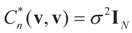 , then
  -covariance of ξ is an (N + K) × (N + K)-matrix given by
  . Here
  is the -covariance of the signal component of ξ. Again, from Assumptions 4.1–4.3 it follows
  that which is the covariance of the signal component of ξ with respect to the limit probability
 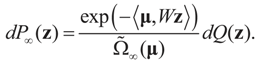 Therefore, φ∞ is also invertible and
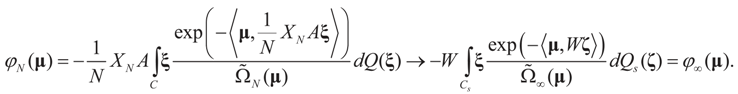
  To verify the uniform convergence of ψN (y) towards ψ∞ (y) note that:


 and
and  are the respective Jacobian matrices. The first order unbiasedness follows by taking expectations,
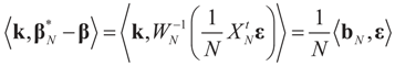
 . Using the representation of lemma 4.5,
  and computing the expected square norm indicated above, we obtain
 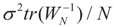 which from Assumption 4.1 tends to 0 as N → ∞.
 ,
,  where
where 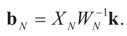 Since the components of ε are i.i.d. random variables, the standard approximations yield:
 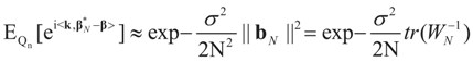 , where
  , and therefore the law of
  concentrates at 0 asymptotically. This completes Part (a).
 factor in the exponent changes the result to be
 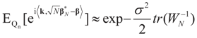 as N → ∞, from which assertion (b) of the proposition follows by the standard continuity theorem.
 Appendix 2: Normal Priors — Derivation of the Basic Linear Model


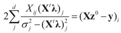
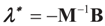
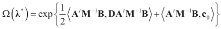
 Solving for λ*,
 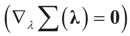 , yields:
 . Explicitly, M is:
 and
and 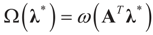 , then following the derivations of Section 3 we get:
 , so:
, so:

 , or
, or 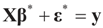 . Under the natural case where the errors’ priors are centered on zero (v0 = 0),
 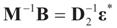 and
and 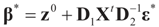 . If in addition z0 = 0, then
 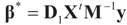 .
.Appendix 3: Model Comparisons — Analytic Examples
 , or only the noise,
  .
.© 2012 by the authors; licensee MDPI, Basel, Switzerland. This article is an open access article distributed under the terms and conditions of the Creative Commons Attribution license (http://creativecommons.org/licenses/by/3.0/).
Share and Cite
Golan, A.; Gzyl, H. An Entropic Estimator for Linear Inverse Problems. Entropy 2012, 14, 892-923. https://doi.org/10.3390/e14050892
Golan A, Gzyl H. An Entropic Estimator for Linear Inverse Problems. Entropy. 2012; 14(5):892-923. https://doi.org/10.3390/e14050892
Chicago/Turabian StyleGolan, Amos, and Henryk Gzyl. 2012. "An Entropic Estimator for Linear Inverse Problems" Entropy 14, no. 5: 892-923. https://doi.org/10.3390/e14050892
APA StyleGolan, A., & Gzyl, H. (2012). An Entropic Estimator for Linear Inverse Problems. Entropy, 14(5), 892-923. https://doi.org/10.3390/e14050892