Optimal Design of ORC Systems with a Low-Temperature Heat Source

Abstract

A numerical model of subcritical and trans-critical power cycles using a fixed-flowrate low-temperature heat source has been validated and used to calculate the combinations of the maximum cycle pressure (P_ev) and the difference between the source temperature and the maximum working fluid temperature (DT) which maximize the thermal efficiency (η_th) or minimize the non-dimensional exergy losses (β), the total thermal conductance of the heat exchangers (UA_t) and the turbine size (SP). Optimum combinations of P_ev and DT were calculated for each one of these four objective functions for two working fluids (R134a, R141b), three source temperatures and three values of the non-dimensional power output. The ratio of UA_t over the net power output (which is a first approximation of the initial cost per kW) shows that R141b is the better working fluid for the conditions under study.

1.Introduction

Considerable quantities of low-temperature thermal energy are available from natural sources (solar, geothermal, biomass) and industrial waste heat (power plants, chemical plants, etc.). In the current context of increasing fossil fuel cost, uncertainty over the safety of nuclear plants and public pressure for the reduction of adverse environmental effects, the conversion of these sources into mechanical energy and electricity is being seriously considered. The methods which can be used to achieve this conversion include systems using organic fluids, mixtures of pure fluids (NH₃/H₂O) and fluids with very low critical temperatures (CO₂). Power plants using such heat sources have been built [1,2] and several manufacturers of plants using an organic Rankine cycle (ORC) announce systems with capacity from 6 kWe to 72 MWe [3]. However, in most cases the published literature consists of semi-analytical or numerical studies.

Liu et al. [4] analyzed the effect of working fluids (wet: water, ethanol; dry: HFE7100, n-pentane, iso-pentane and isentropic: R11, R123, benzene) on the performance of subcritical ORCs and reported that the thermal efficiency of such cycles is a weak function of the critical temperature. They also indicated that using a constant heat source temperature can result in considerable design differences with respect to the actual variable temperature of finite heat sources such as geothermal or waste streams. On the other hand Saleh et al. [5] performed a thermodynamic analysis of 31 pure working fluids for ORCs with and without superheating, operating between 100 and 30 °C. They found that the highest thermal efficiencies are obtained with dry fluids in subcritical cycles with regenerator. They also performed a pinch analysis for the heat transfer between the source and the working fluid and reported that the largest amount of heat can be transferred to a super-critical fluid and the least to a high-boiling subcritical fluid.

Several recent studies present the performance of ORC for conditions which optimize a particular performance indicator with respect to one independent variable. Thus, Lakew and Bolland [6] calculated the value of the evaporator pressure for two design objectives: maximum power output or smallest component size (heat exchanger or turbine). They analyzed a subcritical Rankine cycle without superheating, specified the heat source temperature in the range of 80–200 °C and considered six working fluids (R134a, R123, R227ea, R245fa, R290 and n-pentane). Their results show that the selection of working fluids depends on the type of heat source, the temperature level and the design objective. They concluded that an economic study is necessary to determine which working fluid is the most appropriate. In an analogous study [7] the present authors considered a subcritical Rankine cycle with superheating, operating between a constant flowrate fixed-temperature (100 °C) heat source and a fixed-temperature (10 °C) sink, for five working fluids (R134a, R123, R141b, ammonia and water). These results show the existence of two optimum evaporation temperatures: one minimizes the total thermal conductance of the two heat exchangers whereas the other maximizes the net power output. Based on these results they selected R141b and calculated the minimum thermal conductance for a system generating 686 kW; they also determined the corresponding thermal efficiency (12.6%) and the total exergy losses as a fraction of the source’s exergy (13.8%). Analogously, He et al. [8] considered the evaporation pressure as the independent variable and the net power output as the single objective function. They obtained an analytical expression for the optimum evaporation pressure which maximizes the net power output in the case of a subcritical cycle without superheating and showed that its results are consistent with corresponding numerically predicted values for 22 working fluids. They established that the net power output is larger for working fluids whose critical temperature is close to that of the heat source. For heat source and sink temperatures equal to 150 °C and 20 °C respectively they concluded that R114, R245fa, R123, R601a, n-pentane, R141b and R113 are the most suitable working fluids.

In the present study we extend the previous optimization studies by considering the performance of subcritical and trans-critical systems with two independent variables: the evaporation pressure and the temperature difference between the working and external fluids (source and sink) at the inlet of the latter into the corresponding heat exchanger (evaporator and condenser). Specifically, by considering that the performance of the system is a continuous function of these two independent variables we determine the combinations of their values which maximize the thermal efficiency or minimize the total exergy losses, the total thermal conductance of the two heat exchangers and the turbine size. For each of these conditions the corresponding values of several operating variables (temperature pinch in the evaporator, working fluid mass flowrate, etc.) are determined and analyzed for two working fluids, three heat source temperatures and three non-dimensional power outputs.

2. Description and Model of the System

Figure 1 illustrates the schematic diagram of a basic system used to recover energy from a low temperature gas stream. The heat source is an industrial waste gas idealized as air. It enters the evaporator at a temperature T_s,in with a mass flowrate ${\dot{\text{M}}}_{\text{s}}$. The cooling fluid in the condenser is water with corresponding values T_p,in and ${\dot{\text{M}}}_{\text{p}}$. The working fluid receives heat at a relatively high pressure in the evaporator, expands in a turbine, thereby producing useful work, and rejects heat at a low pressure in the condenser. It is then pumped to the evaporator.

Two possible temperature-entropy diagrams of the system shown in Figure 2a,b illustrate subcritical and trans-critical operation respectively. Even though these figures indicate superheated fluid at the turbine exit it should be noted that for some working fluids and high values of the evaporating pressure state four can be in the two-phase region.

Figure 1. Schematic diagram of system under consideration.

Figure 1. Schematic diagram of system under consideration.

Figure 2. (a) Temperature-entropy diagram of sub-critical system; (b) Temperature-entropy diagram of trans-critical system.

Figure 2. (a) Temperature-entropy diagram of sub-critical system; (b) Temperature-entropy diagram of trans-critical system.

The following assumptions are adopted for the modeling of the system:

• Each component is considered as an open system in steady-state operation;
• Friction and heat losses as well as kinetic and potential energies are neglected;
• The specific heat of the source and sink are assumed to be constant;
• At the exit from the condenser the working fluid is saturated liquid;
• The specific volume of the working fluid remains constant during pumping;
• The efficiency of the turbine and pump is assumed to be constant for all working fluids.

Therefore the first law of thermodynamics for the evaporator, condenser, turbine and pump gives the following relations respectively:

$${\dot{\text{M}}}_{\text{s}}\text{\hspace{0.17em}C}{\mathrm{p}}_{\text{s\hspace{0.17em}}}\left({\text{T}}_{\text{s,in}}-{\text{T}}_{\text{s,out}}\right)=\dot{\text{m}}\left({\text{h}}_3-{\text{h}}_2\right)$$

(1)

$${\dot{\text{M}}}_{\text{p}}\text{\hspace{0.17em}C}{\mathrm{p}}_{\text{p\hspace{0.17em}}}\left({\text{T}}_{\text{p,out}}-{\text{T}}_{\text{p,in}}\right)=\dot{\text{m}}\left({\text{h}}_4-{\text{h}}_1\right)$$

(2)

$$\left({\text{h}}_3-{\text{h}}_4\right)={\mathsf{\eta }}_{\text{T}}\left({\text{h}}_3-{\text{h}}_{\text{4is}}\right)$$

(3)

$${\mathsf{\eta }}_{\text{P}}\left({\text{h}}_2-{\text{h}}_1\right)={\mathsf{\nu }}_1\left({\text{P}}_{\mathrm{ev}}-{\text{P}}_{\mathrm{co}}\right)$$

(4)

Furthermore:

$${\text{s}}_3={\text{ s}}_{\text{4is}},{\text{s}}_{\text{2is}}={\text{ s}}_1$$

(5)

The thermodynamic properties appearing in the above equations are related as follows:

$${\text{h}}_1={\text{ h}}_{\text{sat}}\left({\text{P}}_{\text{co}},{\text{ x}}_1=0\right),{\mathsf{\nu }}_1={\mathsf{\nu }}_{\text{sat}}\left({\text{P}}_{\text{co}},{\text{ x}}_1=0\right)$$

(6a)

$${\text{h}}_3=\text{ h }\left({\text{P}}_{\text{ev}},{\text{ s}}_3\right),{\text{h}}_{\text{4is}}=\text{ h }\left({\text{P}}_{\text{co}},{\text{ s}}_{\text{4is}}\right)$$

(6b)

More equations are obtained by adding the following relations between the temperatures of the working fluid and those of the source and sink:

DT = T_s,in – T₃ = T₁ – T_p,in

(7)

These introduce three more variables (T₃, T₁ and DT) and the following additional relations between thermodynamic properties:

$${\text{P}}_{\text{co}}={\text{ P}}_{\text{sat}}\left({\text{T}}_1\right),{\text{s}}_3=\text{ s }\left({\text{T}}_3,{\text{ P}}_{\text{ev}}\right)$$

(8)

In order to determine whether the conditions at the turbine outlet correspond to superheated vapor or a vapor-liquid mixture the following non-dimensional parameter is introduced:

X₄ = (h₄ – h₁)/(h_g – h₁)

(9a)

where:

$${\text{h}}_{\text{g}}={\text{ h}}_{\text{sat}}\left({\text{P}}_{\text{co}},{\text{ x}}_{\text{g}}=1\right)$$

(9b)

The value of x₄ serves to situate the condenser pinch which is set equal to DT/2. Thus

$$\mathrm{for}{\text{x}}_4<1:{\text{T}}_{\text{p,out}}={\text{ T}}_1-(\text{DT}/2)$$

(10)

$$\mathrm{for}{\text{x}}_4>1:{\text{T}}_{\text{p,pr}}={\text{ T}}_1-(\text{DT}/2)\text{\hspace{0.17em}\hspace{0.17em}\hspace{0.17em}and\hspace{0.17em}\hspace{0.17em}\hspace{0.17em}}{\dot{\text{M}}}_{\text{p}}\text{\hspace{0.17em}C}{\text{p}}_{\text{p}}\left({\text{T}}_{\text{p,pr}}-{\text{T}}_{\text{p,in}}\right)=\dot{\text{m}}\left({\text{h}}_{\text{g}}-{\text{h}}_1\right)$$

(11)

Equations (3)–(8) constitute a system of 11 equations with 17 variables (five temperatures, five enthalpies, two pressures, two entropies, one specific volume and the efficiency of the turbine and pump). Six of these variables must therefore be specified to obtain closure. When this is done the values of the other variables appearing in Equations (3)–(11) can be calculated. The remaining variables appearing in Equations (1) and (2) (the three mass flowrates and T_s,out) can also be calculated if two of them are fixed. We thus obtain the design of a system corresponding to the choice of eight specified variables.

3. Independent Variables, Numerical Solution and Validation

The eight independent variables whose values have been specified during the present study are T_p,in, η_T, η_P, ${\dot{\text{M}}}_{\text{s}}$, T_s,in, P_ev, DT and the net power output of the system. The first four are fixed throughout the present study. The sink temperature T_p,in is set equal to 10 °C (the annual average temperature of the water in the Saint-Lawrence river). The efficiency of the turbine and that of the pump are set equal to 0.8. Based on an actual case the volumetric flowrate of the gaseous source is 1.2 million m³/h (for atmospheric pressure and 100 °C the corresponding mass flowrate is ${\dot{\text{M}}}_{\text{s}}$ = 314.5 kg/s). Its temperature T_s,in can take values between 100 and 230 °C. The range of the temperature difference DT, the evaporation pressure P_ev and the net power output are specified later.

The problem under consideration can therefore be summarized as follows: for the fixed values of T_p,in, η_T, η_P, ${\dot{\text{M}}}_{\text{s}}$ and any value of T_s,in and the net power output in the corresponding specified range, which combination of the other two independent variables, DT and P_ev, optimizes the performance of the system? More specifically the objective is to determine the combination of DT and P_ev which:

(a)

Maximizes the thermal efficiency of the system:

$${\mathsf{\eta }}_{\text{th}}=\left({\dot{\text{W}}}_{\text{T}}-{\dot{\text{W}}}_{\text{P}}\right)/{\dot{\text{Q}}}_{\text{ev}}$$

(12)

where ${\dot{\text{W}}}_{\text{T}}$, ${\dot{\text{W}}}_{\text{P}}$ and ${\dot{\text{Q}}}_{\mathrm{ev}}$ are calculated from Equations (3), (4) and (1) respectively;

(b)

Minimizes the total non-dimensional exergy destruction:

$$\mathsf{\beta }=\left({\dot{\text{E}}}_{\text{d,t}}\right)/\left({\dot{\text{M}}}_{\text{s}}{\text{e}}_{\text{s,in}}\right)$$

(13a)

where the rate of exergy destruction in any of the system’s components is calculated from the exergy balance equation:

$${\dot{\text{E}}}_{\text{d}}={\displaystyle \sum _{\mathrm{in}}({\dot{\text{m}}}_{\mathrm{in}}{\text{e}}_{\mathrm{in}})-}{\displaystyle \sum _{\mathrm{out}}({\dot{\text{m}}}_{\mathrm{out}}{\text{e}}_{\mathrm{out}})-\dot{\text{W}}}$$

(13b)

and the exergy of the working and external fluids at any state can be calculated from:

$$\text{e\hspace{0.17em}\hspace{0.17em}}=(\text{h}-{\text{h}}_0)-{\text{t}}_0(\text{s\hspace{0.17em}}-{\text{s}}_0)$$

(13c)

(c)

Minimizes the total thermal conductance of the two heat exchangers, i.e., the sum of the thermal conductance of each part of the two heat exchangers. For the condenser only one part is considered when x₄ < 1 and the corresponding UA is calculated by dividing the heat transfer rate obtained from Equation (2) by the appropriate logarithmic temperature difference; when x₄ > 1 the thermal conductance for the phase change and desuperheating parts are calculated by dividing the appropriate heat transfer rate [Equation (11b) or the difference of Equations (2) and (11b) respectively] by the corresponding logarithmic temperature difference. For the evaporator a similar procedure is used to calculate the UA value of the three parts (heating of the liquid from 2 to 2*, evaporation from 2* to 3* and superheating from 3* to 4) for subcritical operation (Figure 2a) or of the 20 parts into which the process from 2 to 3 is subdivided for trans-critical operation (Figure 2b). This approach has been used by Lakew and Bolland [6] and Cayer et al. [9].

(d)

Minimizes the turbine size parameter SP which accounts for the actual turbine dimensions [10] and is calculated from:

$$\text{SP\hspace{0.17em}\hspace{0.17em}}={({\text{V}}_{\text{T,4is}})}^{0.5}/{(1000\Delta {\text{h}}_{\mathrm{is}})}^{0.25}$$

(14)

The values of DT considered in the present study are between 5 and 25 °C except as noted in one particular case. It is important to distinguish between this variable and the temperature pinch in the heat exchangers. Thus, in the condenser the pinch is equal to DT/2 and occurs at the position where the working fluid is saturated vapor when x₄ ≥ 1 or at the sink outlet when x₄ < 1. In the evaporator, for small glides of the source temperature the pinch occurs at the source inlet and is equal to DT; for large glides of the source temperature it occurs at the position where the working fluid is saturated liquid in the case of a subcritical cycle and at a position intermediate between the inlet and outlet of the evaporator in the case of a trans-critical cycle. In the latter case this position can be determined by subdividing the evaporator in a large number of segments and by applying the first law of thermodynamics [9]. During the present study combinations of the independent variables resulting in an evaporator pinch lower than DT/2 have been disregarded since they lead to large values of the evaporator thermal conductance.

The range of evaporator pressures examined during the present study is also bounded. Its lowest value is equal to the condenser pressure which is determined from T_p,in and DT [using Equation (7) to obtain T₁ and Equation (8)]. For subcritical operation (Figure 2a) its highest accepted value is equal to the saturation pressure corresponding to T₃ [obtained from Equation (7)] while for trans-critical operation (Figure 2b) it is equal to the pressure corresponding to the temperature of state 3 (T₃) and the entropy of the critical state (s_cr). However it should be noted that this upper limit is seldom reached since it is required that the quality at the turbine outlet should not be lower than 0.95 to avoid problems caused by liquid droplets in the turbine.

The model of the system was solved using the EES code [11] which includes thermodynamic properties for a large number of natural and manufactured fluids. The present model and calculation procedure were successfully validated by comparing their results with corresponding results from the literature. Figure 3 shows the thermal efficiency of an ideal Rankine cycle (η_T = η_p = 1), using HCFC 123 as the working fluid, calculated by the present code and corresponding results by Madhawa Hettiarachchi et al. [12] who have shown that their results agree perfectly with those obtained by Liu et al. [4]. The agreement between the present results and those of the two other studies is excellent for the entire range of turbine inlet temperatures. Further comparisons published elsewhere by Khennich and Galanis [7] confirm the validity of the present model and solution methodology.

The optimization of the functions η(DT, P_ev), β(DT, P_ev), UA_t(DT, P_ev) and SP(DT, P_ev) for the specified range of the independent variables DT and P_ev was carried out using the Variable Metric method for multi-dimensional optimization which is included in EES. According to the EES manual this method, which uses numerical derivatives, performs much better than the Direct Search method.

Figure 3. Comparison of present results with those by Madhawa Hettiarachchi [12] for an ideal Rankine cycle using HCFC 123 and a condenser temperature of 303 K.

Figure 3. Comparison of present results with those by Madhawa Hettiarachchi [12] for an ideal Rankine cycle using HCFC 123 and a condenser temperature of 303 K.

4. Working Fluids

The choice of the working fluids was based on their thermodynamic and environmental characteristics. Working fluids for systems with low or intermediate temperature sources must satisfy several safety, environmental, performance and economic criteria [13]. Among the safety aspects, flammability, toxicity and auto-ignition are particularly important. Environmental criteria include the ozone depletion potential (ODP) and the global warming potential (GWP). Based on these considerations R134a and R141b, which have been included in several recent studies [6,8,14,15,16], are used in the present study. Their thermophysical, safety and environmental properties are presented and compared in Table 1. From a safety point of view R141b has a lower flammability while R134a has no flame propagation. It should be noted however that R141b will be phased out by 2030 due to its non-zero ODP [13] and that the stability of these two fluids at relatively high temperatures and pressures has not been established. Therefore results for such conditions are only included to illustrate the proposed optimization methodology and to establish the influence of the independent variables DT and P_ev on the values of the four design parameters defined in the previous section (η_th, β, UA and SP).

Table 1. Thermophysical, environmental and safety characteristics of working fluids.

Fluid	Formula	Mol. weight (kg/kmol)	NBP (°C)	Tcr (°C)	Pcr (MPa)	ASHRAE 34 safety	ODP	GWP	Nature
R134a	CH2FCF3	102.03	−26.1	101.03	4.06	A1	0	1300	Isentropic
R141b	CH3CCl2F	116.95	32.0	204.20	4.25	A2	0.086	700	Isentropic

Table 1. Thermophysical, environmental and safety characteristics of working fluids.

Fluid	Formula	Mol. weight (kg/kmol)	NBP (°C)	Tcr (°C)	Pcr (MPa)	ASHRAE 34 safety	ODP	GWP	Nature
R134a	CH2FCF3	102.03	−26.1	101.03	4.06	A1	0	1300	Isentropic
R141b	CH3CCl2F	116.95	32.0	204.20	4.25	A2	0.086	700	Isentropic

EES calculates the thermodynamic properties using the equation of state developed by Tillner-Roth and Baehr [17] for R134a and the one provided by Martin-Hou [18] for R141b.

5. Results and Discussion

The results presented here have been calculated for the previously mentioned two working fluids with the four fixed variables (${\dot{\text{M}}}_{\text{s}}$ = 314.5 kg/s, T_p,in = 10 °C, ηT = ηP = 0.8), three different source temperatures (T_s,in = 100, 165 and 230 °C) and three different values of the non-dimensional net power output α which is obtained by dividing (${\dot{\text{W}}}_{\text{T}}–{\dot{\text{W}}}_{\text{P}}$) by the following reference power:

$${\dot{\text{W}}}_{\mathrm{ref}}={\dot{\text{M}}}_{\text{s}}\text{\hspace{0.17em}C}{\text{p}}_{\text{s\hspace{0.17em}}}\left({\text{T}}_{\text{s,in}}-{\text{T}}_{\text{p,in}}\right)\left[1-\left({\text{T}}_{\text{p,in}}/{\text{T}}_{\text{s,in}}\right)\right]$$

(15)

${\dot{\text{W}}}_{\mathrm{ref}}$ is evaluated by considering a Carnot process operating between the inlet temperatures of the heat source and sink. The product of the mass flowrate, the specific heat and the temperature difference is higher than the actual heat extracted from the heat source while the Carnot efficiency is higher than that of the actual cycle using the specified heat source and sink. Therefore the values of (α) are considerably lower than one (Khennich and Galanis [7], Cayer et al. [9]). In the present study the adopted values of (α) are 0.04, 0.08 and 0.12. The range of values for the temperature difference DT and the evaporation pressure P_ev has been specified in Section 3.

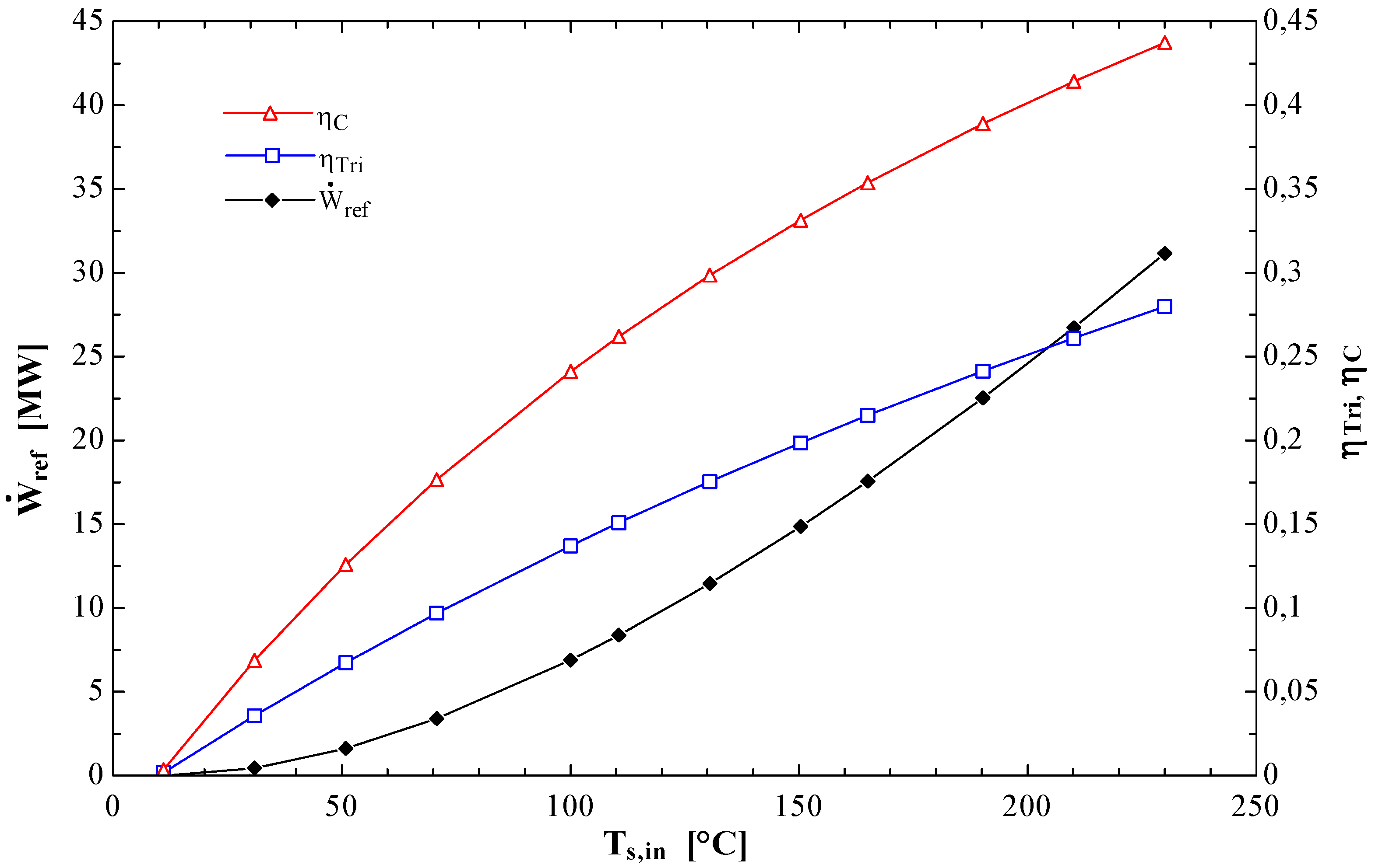
Figure 4 shows the effect of the inlet source temperature on the reference power as well as on the Carnot (η_C) and triangular (η_Tri) cycle efficiencies. The latter, which is considered to be a more realistic upper limit than the Carnot efficiency for trans-critical cycles is calculated from the following expression (Schuster et al. [14]):

$${\mathsf{\eta }}_{\text{Tri}}=({\text{t}}_{\text{s,in}}-{\text{t}}_{\text{p,in}})/({\text{t}}_{\text{s,in}}+{\text{t}}_{\text{p,in}})$$

(16a)

$${\mathsf{\eta }}_{\text{C }}=1-({\text{t}}_{\text{p,in}}/{\text{t}}_{\text{s,in}})$$

(16b)

Figure 4. Effect of T_s,in on the reference power, the Carnot efficiency and the triangular efficiency.

Figure 4. Effect of T_s,in on the reference power, the Carnot efficiency and the triangular efficiency.

The results of Figure 4 show that these three quantities which are independent of the working fluid increase non-linearly with T_s,in. All three are equal to zero when T_s,in is equal to T_p,in; as T_s,in increases the reference power tends to infinity while the Carnot and triangular efficiencies approach unity. A comparison of the cycle’s thermal efficiency calculated from Equation (12) with the two values obtained from Equations (16a) and (16b) would give a clear indication of the thermodynamic performance of the system under study. However, since the thermal efficiency can be interpreted as the ratio of revenues (which are proportional to the net power output) to running costs (which are to a large extent proportional to the rate of heat input) it is not a very important performance criterion for systems which use a free source of heat (waste or solar or geothermal heat). In such cases an economic analysis is required to select an optimum design as pointed out by Lakew and Bolland [6]. Such an analysis requires the specification of several details (for example: the diameter of the tubes and the shell in a tube and shell heat exchanger, see [9]) and lacks the generality aimed for in the present study. Instead we introduce the following non-dimensional parameter which combines the total thermal conductance of the heat exchangers and the net power output:

$$\text{F }={\text{ UA}}_{\text{t}}\left({\text{T}}_{\text{s,in}}-{\text{T}}_{\text{p,in}}\right)/\left({\dot{\text{W}}}_{\text{T}}-{\dot{\text{W}}}_{\text{P}}\right)$$

(17)

The total thermal conductance of the heat exchangers, UA_t, is considered to represent the initial cost of the system. It is of course true that this cost depends on other variables, e.g., the operating pressures and the turbine size SP. However, it is shown later that, for a fixed combination of source temperature and net power output, SP does not depend much on the design criterion while the opposite is true for UA_t. Therefore the initial cost will depend more on the latter variable. On the other hand the denominator of F [Equation (17)] determines the revenues generated by the system. In view of the above discussion we believe that this parameter is more appropriate than the thermal efficiency for the comparison of systems using free sources of heat since low values of F likely correspond to a smaller initial cost per kW or a higher output (higher revenues) for a given investment. It should also be noted that the ratio of total heat transfer area A to the net power output (Ẇ_T − Ẇ_P) was used as an optimization criterion in the study by Madhawa Hettiarachchi et al. [12]. That ratio lacks the generality of the parameter F used in the present study since it is dimensional and its calculation requires the specification of additional information regarding the heat exchangers. Specifically the type of heat exchanger (plate, shell and tubes, etc.), the size of its parts as well as correlations for the calculation of heat transfer coefficients are the minimum requirements for the evaluation of U as illustrated in [12] and [19].

5.1. Results for R134a

Table 2 shows the optimization results for R134a and a source temperature of 100 °C. Part 2.1 presents the maximum thermal efficiency, the operating conditions (P_ev,opt and DT_opt) for which this maximum efficiency is attained as well as the corresponding values of several other parameters. We note that in this case the optimum evaporation pressure is equal to the highest value compatible with the imposed constraints and that the optimum temperature difference DT is equal to the lower limit of the adopted range. As expected the maximum efficiency of this subcritical cycle is lower than the corresponding Carnot (η_C = 24.1%) and triangular (η_Tri = 13.7%) efficiencies. Its value and the operating conditions for which it is attained are independent of the non-dimensional power output. On the other hand the non-dimensional exergy destruction, the total thermal conductance, the turbine size parameter and the working fluid mass flowrate increase monotonically with the non-dimensional power output. In fact $\dot{\text{m}}$ increases linearly with α while the rate of increase of β and SP decreases as (α) increases and that of UA_t increases with (α). For all the values of (α) the working fluid is superheated at the turbine outlet (x₄ > 1) while the evaporator pinch occurs at the inlet of the source and is therefore always equal to DT_opt. For these conditions the value of F [Equation (17)] increases with the non-dimensional power output indicating that the initial cost per kW likely decreases as the net power output decreases.

Part 2.2 of Table 2 shows that the minimum non-dimensional total exergy destruction is obtained for the same operating conditions (P_ev,opt and DT_opt) which maximize the thermal efficiency. Therefore the values of all the other calculated variables in Parts 2.1 and 2.2 are identical. This result establishes the fact that for this source temperature it is possible to simultaneously maximize the thermal efficiency and minimize the total exergy destruction.

Part 2.3 of Table 2 presents the minimum total thermal conductance of the heat exchangers, the operating conditions (P_ev,opt and DT_opt) for which this thermal conductance is attained as well as the corresponding values of other calculated parameters. For a given value of (α) the minimum thermal conductance is approximately 45% lower than the one corresponding to maximum thermal efficiency and minimum exergy destruction. However, this important reduction of the heat exchangers’ conductance is accompanied by a significant deterioration of the other calculated parameters. Thus, the thermal efficiency decreases by approximately 30%, the total exergy destruction increases by approximately 60%, the working fluid mass flowrate and turbine size increase by approximately 75% and 10% respectively. These results establish a fact observed throughout this study, i.e., that for a given combination of T_s,in and (α) (or equivalently a fixed net power output) the influence of different design scenarios on the variation of SP is rather small compared to that of UA_t. It therefore justifies the assertion that the numerator of Equation (17) determines to a considerable degree the initial cost of the system. The results of Part 2.3 show that the values of F obtained by minimizing UA_t are approximately half of the corresponding values in Parts 2.1 and 2.2 of the Table indicating that the minimization of UA_t leads to systems requiring a smaller initial investment for a given power output.

Table 2. Optimization of the ORC with R134a for T_s,in = 100 °C (sub-critical), DT between 5 and 25 °C (η_C = 24.1%, η_Tri = 13.7%, ${\dot{\text{W}}}_{\text{ref}}$ = 6897 kW).

[2.1] α	ηth,max	Pev,opt	DTopt	β	UAt	SP	$\dot{\mathbf{\text{m}}}$	x4	Pinchev	F
	%	(kPa)	(°C)	%	(kW/K)	(m)	(kg/s)		(°C)
0.04	11.26	2365.0	5.00	7.64	662.3	0.0502	10.376	1.122	5.00	216.1
0.08	11.26	2365.0	5.00	14.19	1351.5	0.0710	20.753	1.122	5.00	220.4
0.12	11.26	2365.0	5.00	19.61	2087.3	0.0870	31.129	1.122	5.00	227.0
[2.2] α	βmin	Pev,opt	DTopt	ηth	UAt	SP	$\dot{\mathbf{\text{m}}}$	x4	Pinchev	F
	%	(kPa)	(°C)	%	(kW/K)	(m)	(kg/s)		(°C)
0.04	7.64	2365.0	5.00	11.26	662.3	0.0502	10.376	1.122	5.00	216.1
0.08	14.19	2365.0	5.00	11.26	1351.5	0.0710	20.753	1.122	5.00	220.4
0.12	19.61	2365.0	5.00	11.26	2087.3	0.0870	31.129	1.122	5.00	227.0
[2.3] α	UAt,min	Pev,opt	DTopt	β	ηth	SP	$\dot{\mathbf{\text{m}}}$	x4	Pinchev	F
	(kW/K)	(kPa)	(°C)	%	%	(m)	(kg/s)		(°C)
0.04	341.0	2365.0	21.69	12.09	8.07	0.0559	18.101	1.012	18.09	111.2
0.08	749.0	2320.9	18.80	20.54	8.55	0.0773	32.504	1.042	12.71	122.2
0.12	1268.3	2205.5	15.91	26.93	8.84	0.0945	44.678	1.079	8.57	137.9
[2.4] α	SPmin	Pev,opt	DTopt	β	ηth	UAt	$\dot{\mathbf{\text{m}}}$	x4	Pinchev	F
	(m)	(kPa)	(°C)	%	%	(kW/K)	(kg/s)		(°C)
0.04	0.0502	2365.0	5.00	7.64	11.26	662.3	10.376	1.122	5.00	216.1
0.08	0.0710	2365.0	5.00	14.19	11.26	1351.5	20.753	1.122	5.00	220.4
0.12	0.0870	2365.0	5.00	19.61	11.26	2087.3	31.129	1.122	5.00	227.0

Table 2. Optimization of the ORC with R134a for T_s,in = 100 °C (sub-critical), DT between 5 and 25 °C (η_C = 24.1%, η_Tri = 13.7%, ${\dot{\text{W}}}_{\text{ref}}$ = 6897 kW).

[2.1] α	ηth,max	Pev,opt	DTopt	β	UAt	SP	$\dot{\mathbf{\text{m}}}$	x4	Pinchev	F
	%	(kPa)	(°C)	%	(kW/K)	(m)	(kg/s)		(°C)
0.04	11.26	2365.0	5.00	7.64	662.3	0.0502	10.376	1.122	5.00	216.1
0.08	11.26	2365.0	5.00	14.19	1351.5	0.0710	20.753	1.122	5.00	220.4
0.12	11.26	2365.0	5.00	19.61	2087.3	0.0870	31.129	1.122	5.00	227.0
[2.2] α	βmin	Pev,opt	DTopt	ηth	UAt	SP	$\dot{\mathbf{\text{m}}}$	x4	Pinchev	F
	%	(kPa)	(°C)	%	(kW/K)	(m)	(kg/s)		(°C)
0.04	7.64	2365.0	5.00	11.26	662.3	0.0502	10.376	1.122	5.00	216.1
0.08	14.19	2365.0	5.00	11.26	1351.5	0.0710	20.753	1.122	5.00	220.4
0.12	19.61	2365.0	5.00	11.26	2087.3	0.0870	31.129	1.122	5.00	227.0
[2.3] α	UAt,min	Pev,opt	DTopt	β	ηth	SP	$\dot{\mathbf{\text{m}}}$	x4	Pinchev	F
	(kW/K)	(kPa)	(°C)	%	%	(m)	(kg/s)		(°C)
0.04	341.0	2365.0	21.69	12.09	8.07	0.0559	18.101	1.012	18.09	111.2
0.08	749.0	2320.9	18.80	20.54	8.55	0.0773	32.504	1.042	12.71	122.2
0.12	1268.3	2205.5	15.91	26.93	8.84	0.0945	44.678	1.079	8.57	137.9
[2.4] α	SPmin	Pev,opt	DTopt	β	ηth	UAt	$\dot{\mathbf{\text{m}}}$	x4	Pinchev	F
	(m)	(kPa)	(°C)	%	%	(kW/K)	(kg/s)		(°C)
0.04	0.0502	2365.0	5.00	7.64	11.26	662.3	10.376	1.122	5.00	216.1
0.08	0.0710	2365.0	5.00	14.19	11.26	1351.5	20.753	1.122	5.00	220.4
0.12	0.0870	2365.0	5.00	19.61	11.26	2087.3	31.129	1.122	5.00	227.0

Finally, Part 2.4 of Table 2 shows that the minimum turbine size is obtained for the same operating conditions (P_ev,opt and DT_opt) which maximize the thermal efficiency and minimize the non-dimensional total exergy destruction. Therefore the values of all the other calculated variables in Parts 2.1, 2.2 and 2.4 are identical. This result is important since it establishes the fact that for this source temperature it is possible to simultaneously maximize the thermal efficiency and minimize the total exergy destruction as well as the turbine size. The corresponding combination of P_ev = 2365 kPa and DT = 5 °C constitutes an interesting design condition for T_s,in = 100 °C. However such a system is likely quite costly since the corresponding total thermal conductance is approximately twice the minimum value given in Part 2.3 of Table 2.

Analogous results for a trans-critical cycle with a source temperature of 165 °C are presented in Table 3. They show that in this case the operating conditions which maximize the thermal efficiency, minimize the total exergy destruction and minimize the turbine size are not identical. The difference between the conditions which maximize the thermal efficiency and those which minimize the exergy destruction are small (same optimum DT, small differences in optimum P_ev). On the other hand the conditions minimizing the turbine size are significantly different (smaller optimum evaporation pressures and higher values of DT). However, for a given value of (α) (or equivalently a fixed net power output) the maximum value of SP in the four parts of Table 3 is within 5% of its minimum while the corresponding maximum for UA_t is 249% of its minimum. The values of F for the conditions minimizing UA_t (Part 3.3) are even lower than those obtained for T_s,in = 100 °C (see Part 2.3 of Table 2) indicating that the initial cost per kW of such optimum systems probably decreases as the source temperature increases. The uncertainty in this last statement is due to two factors. First, the initial cost of the system increases with the area A of the heat exchangers rather than their thermal conductance UA. Second, the value of F does not take into account the higher cost resulting from the increase of the evaporation pressure corresponding to that of the heat source temperature (c.f. Table 2 and Table 3).

Table 3. Optimization of the ORC cycle with R134a for T_s,in = 165 °C (trans-critical), DT between 5 and 25 °C (η_C = 35.4%, η_Tri = 21.5%, ${\dot{\text{W}}}_{\text{ref}}$ = 17565 kW).

[3.1] α	ηth,max	Pev,opt	DTopt	β	UAt	SP	$\dot{\mathbf{\text{m}}}$	x4	Pinchev	F
	%	(kPa)	(°C)	%	(kW/K)	(m)	(kg/s)		(°C)
0.04	15.94	7120.9	5.00	7.96	1044.7	0.0568	16.882	1.176	5.00	230.5
0.08	15.94	7120.9	5.00	14.93	2115.3	0.0803	33.764	1.176	5.00	233.3
0.12	15.94	7120.9	5.00	20.87	3222.2	0.0984	50.646	1.176	5.00	236.9
[3.2] α	βmin	Pev,opt	DTopt	ηth	UAt	SP	$\dot{\mathbf{\text{m}}}$	x4	Pinchev	F
	%	(kPa)	(°C)	%	(kW/K)	(m)	(kg/s)		(°C)
0.04	7.96	7081.6	5.00	15.94	1042.9	0.0568	16.849	1.178	5.00	230.1
0.08	14.93	7078.6	5.00	15.94	2111.3	0.0803	33.694	1.178	5.00	232.9
0.12	20.87	7075.0	5.00	15.94	3215.5	0.0984	50.531	1.178	5.00	236.5
[3.3] α	UAt,min	Pev,opt	DTopt	β	ηth	SP	$\dot{\mathbf{\text{m}}}$	x4	Pinchev	F
	(kW/K)	(kPa)	(°C)	%	%	(m)	(kg/s)		(°C)
0.04	390.6	4968.1	25.00	11.84	11.84	0.0589	25.936	1.199	25.00	86.2
0.08	814.5	4968.1	25.00	21.86	11.84	0.0833	51.871	1.199	25.00	89.8
0.12	1295.0	4968.1	25.00	29.87	11.84	0.1019	77.863	1.197	25.00	95.2
[3.4] α	SPmin	Pev,opt	DTopt	β	ηth	UAt	$\dot{\mathbf{\text{m}}}$	x4	Pinchev	F
	(m)	(kPa)	(°C)	%	%	(kW/K)	(kg/s)		(°C)
0.04	0.0565	6428.5	10.47	8.76	14.88	600.5	18.678	1.183	10.47	132.5
0.08	0.0800	6428.7	10.47	16.39	14.88	1225.4	37.358	1.183	10.47	135.2
0.12	0.0979	6429.1	10.47	22.81	14.88	1886.1	56.033	1.183	10.47	138.7

Table 3. Optimization of the ORC cycle with R134a for T_s,in = 165 °C (trans-critical), DT between 5 and 25 °C (η_C = 35.4%, η_Tri = 21.5%, ${\dot{\text{W}}}_{\text{ref}}$ = 17565 kW).

[3.1] α	ηth,max	Pev,opt	DTopt	β	UAt	SP	$\dot{\mathbf{\text{m}}}$	x4	Pinchev	F
	%	(kPa)	(°C)	%	(kW/K)	(m)	(kg/s)		(°C)
0.04	15.94	7120.9	5.00	7.96	1044.7	0.0568	16.882	1.176	5.00	230.5
0.08	15.94	7120.9	5.00	14.93	2115.3	0.0803	33.764	1.176	5.00	233.3
0.12	15.94	7120.9	5.00	20.87	3222.2	0.0984	50.646	1.176	5.00	236.9
[3.2] α	βmin	Pev,opt	DTopt	ηth	UAt	SP	$\dot{\mathbf{\text{m}}}$	x4	Pinchev	F
	%	(kPa)	(°C)	%	(kW/K)	(m)	(kg/s)		(°C)
0.04	7.96	7081.6	5.00	15.94	1042.9	0.0568	16.849	1.178	5.00	230.1
0.08	14.93	7078.6	5.00	15.94	2111.3	0.0803	33.694	1.178	5.00	232.9
0.12	20.87	7075.0	5.00	15.94	3215.5	0.0984	50.531	1.178	5.00	236.5
[3.3] α	UAt,min	Pev,opt	DTopt	β	ηth	SP	$\dot{\mathbf{\text{m}}}$	x4	Pinchev	F
	(kW/K)	(kPa)	(°C)	%	%	(m)	(kg/s)		(°C)
0.04	390.6	4968.1	25.00	11.84	11.84	0.0589	25.936	1.199	25.00	86.2
0.08	814.5	4968.1	25.00	21.86	11.84	0.0833	51.871	1.199	25.00	89.8
0.12	1295.0	4968.1	25.00	29.87	11.84	0.1019	77.863	1.197	25.00	95.2
[3.4] α	SPmin	Pev,opt	DTopt	β	ηth	UAt	$\dot{\mathbf{\text{m}}}$	x4	Pinchev	F
	(m)	(kPa)	(°C)	%	%	(kW/K)	(kg/s)		(°C)
0.04	0.0565	6428.5	10.47	8.76	14.88	600.5	18.678	1.183	10.47	132.5
0.08	0.0800	6428.7	10.47	16.39	14.88	1225.4	37.358	1.183	10.47	135.2
0.12	0.0979	6429.1	10.47	22.81	14.88	1886.1	56.033	1.183	10.47	138.7

Analogous results have been calculated for a trans-critical cycle with a source temperature of 230 °C. They confirm the trends discussed above but are not presented because R134a may not be stable at the corresponding high temperatures and pressures.

By comparing these results the following comments can be formulated:

• The maximum thermal efficiency (Part 1 of the Tables) is independent of the net power output and increases with T_s,in. The corresponding optimum evaporation pressure also increases with T_s,in while the corresponding optimum value of DT is always equal to the smallest value in the chosen range.
• The minimum non-dimensional exergy losses (Part 2 of the Tables), the minimum total thermal conductance of the heat exchangers (Part 3 of the Tables) and the minimum turbine size (Part 4 of the Tables) increase with the net power output and with T_s,in.
• The conditions (P_ev and DT) which minimize the non-dimensional exergy losses are essentially the same as those which maximize the thermal efficiency.
• The proposed performance indicator F (which provides a first approximation of the initial cost per unit net output) increases with the net power output. For any given source temperature the lowest values of F are obtained for the conditions which minimize UA_t. These lowest values of F decrease as T_s,in increases.
• At the exit from the turbine the working fluid is always superheated. In the case of the trans-critical cycle with T_s,in = 230 °C, for which the superheating is most important, the use of regeneration may be advisable.
• For the conditions maximizing the thermal efficiency (Part 1 of the Tables) and those minimizing the non-dimensional exergy losses (Part 2 of the Tables), the total thermal conductance of the heat exchangers (Part 3 of the Tables) and the turbine size (Part 4 of the Tables) the evaporator pinch is equal to the corresponding optimum value of DT (with the exception of Part 3 of Table 2) and occurs at the inlet of the heat source in most cases.

5.2. Results for R141b

Table 4, Table 5, Table 6 and Table 7 show analogous results for this second working fluid which has a considerably higher critical temperature than R134a (see Table 1). Thus Table 4 and Table 5 for T_s,in equal to 100 and 165 °C respectively correspond to a sub-critical cycle. In the case of T_s,in = 230 °C sub-critical and trans-critical results are presented in Table 6 and Table 7 respectively; the latter were obtained by increasing the range of DT to 30–50 °C. By comparing the results in these Tables the following comments can be formulated:

• The maximum thermal efficiency (Part 1 of Table 4, Table 5, Table 6 and Table 7 ) is independent of the net power output and increases with T_s,in. For T_s,in = 230 °C the trans-critical cycle has a better thermal efficiency than the sub-critical one. The corresponding optimum evaporation pressure also increases with T_s,in and is highest for the trans-critical cycle with T_s,in = 230 °C; the corresponding optimum value of DT is always equal to the smallest value in the chosen range.
• The minimum non-dimensional exergy losses (Part 2 of Table 4, Table 5, Table 6 and Table 7) increase with the net power output and with T_s,in. The lowest minimum exergy losses are obtained for T_s,in = 165 °C. In the case with T_s,in = 230 °C the trans-critical cycle has a lower β_min than the sub-critical cycle.
• The conditions (P_ev and DT) which minimize the non-dimensional exergy losses are essentially the same as those which maximize the thermal efficiency.
• The minimum total thermal conductance of the heat exchangers (Part 3 of Table 4, Table 5, Table 6 and Table 7) increases with the non-dimensional power output. When α = 0.04 UA_t is lowest for T_s,in = 100 °C followed by the sub-critical cycle with T_s,in = 230 °C. When α = 0.12 it is lowest for the sub-critical cycle with T_s,in = 230 °C followed by the cycle with T_s,in = 165 °C.
• The minimum turbine size (Part 4 of Table 4, Table 5, Table 6 and Table 7) increases with the non-dimensional power output. The smallest values of SP_min are obtained for the sub-critical cycle with T_s,in = 230 °C.
• At the exit from the turbine the fluid is always superheated.
• For any of the four cycles under consideration the working fluid mass flowrate is lowest for the conditions which maximize η_th and minimize β; it is highest for the conditions minimizing UA_t and increases with the net power output.
• For the conditions maximizing η_th and minimizing β the pinch in the evaporator is equal to the smallest value of DT in the chosen range and occurs at the inlet of the source (except for the sub-critical cycle with T_s,in = 230 °C and α = 0.12). For the conditions minimizing UA_t and SP the evaporator pinch has a value higher than the smallest value of DT.
• The conditions minimizing UA_t give turbines which are not much bigger than the corresponding smallest one. On the other hand the conditions which minimize SP give very high values of UA_t compared to their minimum values. It is therefore justified to base a preliminary design on the conditions which minimize UA_t and to use the proposed performance criterion F [see Equation (17)] as an indicator of the specific cost of the system.
• The value of F increases with the non-dimensional power output and its lowest values are obtained for the conditions which minimize UA_t as in the case of R134a. For any given combination of T_s,in and (α) the lowest values of F and the corresponding evaporation pressure are smaller in the case of R141b suggesting a lower initial cost per unit output for systems using this working fluid. The subcritical cycle with T_s,in = 230 °C designed for the operating conditions which minimize UA_t has the lowest values of F among all the cases included in Table 2, Table 3, Table 4, Table 5, Table 6 and Table 7.

Table 4. Optimization of the ORC cycle with R141b for T_s,in = 100 °C (sub-critical), DT between 5 and 25 °C (η_C = 24.1%, η_Tri = 13.7%, ${\dot{\text{W}}}_{\text{ref}}$ = 6897 kW).

[4.1] α	ηth,max	Pev,opt	DTopt	β	UAt	SP	$\dot{\mathbf{\text{m}}}$	x4	Pinchev	F
	%	(kPa)	(°C)	%	(kW/K)	(m)	(kg/s)		(°C)
0.04	12.18	371.3	5.00	6.56	612.7	0.1220	7.822	1.100	5.00	199.9
0.08	12.18	371.3	5.00	12.19	1255.4	0.1725	15.644	1.100	5.00	204.8
0.12	12.10	366.0	5.00	17.08	1958.8	0.2124	23.609	1.101	5.00	213.0
[4.2] α	βmin	Pev,opt	DTopt	ηth	UAt	SP	$\dot{\mathbf{\text{m}}}$	x4	Pinchev	F
	%	(kPa)	(°C)	%	(kW/K)	(m)	(kg/s)		(°C)
0.04	6.56	371.3	5.00	12.18	612.7	0.1220	7.822	1.100	5.00	199.9
0.08	12.19	371.3	5.00	12.18	1255.4	0.1725	15.644	1.100	5.00	204.8
0.12	17.08	366.0	5.00	12.10	1958.8	0.2124	23.609	1.101	5.00	213.0
[4.3] α	UAt,min	Pev,opt	DTopt	β	ηth	SP	$\dot{\mathbf{\text{m}}}$	x4	Pinchev	F
	(kW/K)	(kPa)	(°C)	%	%	(m)	(kg/s)		(°C)
0.04	315.3	371.3	21.29	10.14	9.02	0.1224	11.920	1.043	17.39	102.9
0.08	702.5	359.2	18.57	17.83	9.35	0.1746	22.489	1.056	11.60	114.6
0.12	1217.1	331.1	15.43	24.28	9.48	0.2211	32.404	1.076	7.46	132.4
[4.4] α	SPmin	Pev,opt	DTopt	β	ηth	UAt	x4	$\dot{\mathbf{\text{m}}}$	Pinchev	F
	(m)	(kPa)	(°C)	%	%	(kW/K)	(kg/s)		(°C)
0.04	0.1205	371.3	12.86	8.03	10.65	351.9	9.459	1.074	12.86	114.8
0.08	0.1704	371.3	12.86	14.83	10.65	749.7	18.918	1.074	12.47	122.3
0.12	0.2101	366.0	12.51	20.47	10.64	1260.6	28.330	1.076	6.69	137.1

Table 4. Optimization of the ORC cycle with R141b for T_s,in = 100 °C (sub-critical), DT between 5 and 25 °C (η_C = 24.1%, η_Tri = 13.7%, ${\dot{\text{W}}}_{\text{ref}}$ = 6897 kW).

[4.1] α	ηth,max	Pev,opt	DTopt	β	UAt	SP	$\dot{\mathbf{\text{m}}}$	x4	Pinchev	F
	%	(kPa)	(°C)	%	(kW/K)	(m)	(kg/s)		(°C)
0.04	12.18	371.3	5.00	6.56	612.7	0.1220	7.822	1.100	5.00	199.9
0.08	12.18	371.3	5.00	12.19	1255.4	0.1725	15.644	1.100	5.00	204.8
0.12	12.10	366.0	5.00	17.08	1958.8	0.2124	23.609	1.101	5.00	213.0
[4.2] α	βmin	Pev,opt	DTopt	ηth	UAt	SP	$\dot{\mathbf{\text{m}}}$	x4	Pinchev	F
	%	(kPa)	(°C)	%	(kW/K)	(m)	(kg/s)		(°C)
0.04	6.56	371.3	5.00	12.18	612.7	0.1220	7.822	1.100	5.00	199.9
0.08	12.19	371.3	5.00	12.18	1255.4	0.1725	15.644	1.100	5.00	204.8
0.12	17.08	366.0	5.00	12.10	1958.8	0.2124	23.609	1.101	5.00	213.0
[4.3] α	UAt,min	Pev,opt	DTopt	β	ηth	SP	$\dot{\mathbf{\text{m}}}$	x4	Pinchev	F
	(kW/K)	(kPa)	(°C)	%	%	(m)	(kg/s)		(°C)
0.04	315.3	371.3	21.29	10.14	9.02	0.1224	11.920	1.043	17.39	102.9
0.08	702.5	359.2	18.57	17.83	9.35	0.1746	22.489	1.056	11.60	114.6
0.12	1217.1	331.1	15.43	24.28	9.48	0.2211	32.404	1.076	7.46	132.4
[4.4] α	SPmin	Pev,opt	DTopt	β	ηth	UAt	x4	$\dot{\mathbf{\text{m}}}$	Pinchev	F
	(m)	(kPa)	(°C)	%	%	(kW/K)	(kg/s)		(°C)
0.04	0.1205	371.3	12.86	8.03	10.65	351.9	9.459	1.074	12.86	114.8
0.08	0.1704	371.3	12.86	14.83	10.65	749.7	18.918	1.074	12.47	122.3
0.12	0.2101	366.0	12.51	20.47	10.64	1260.6	28.330	1.076	6.69	137.1

Table 5. Optimization of the ORC cycle with R141b for T_s,in = 165 °C (sub-critical), DT between 5 and 25 °C (η_C = 35.4%, η_Tri = 21.5%, ${\dot{\text{W}}}_{\text{ref}}$ = 17565 kW).

[5.1] α	ηth,max	Pev,opt	DTopt	β	UAt	SP	$\dot{\mathbf{\text{m}}}$	x4	Pinchev	F
	%	(kPa)	(°C)	%	(kW/K)	(m)	(kg/s)		(°C)
0.04	19.06	1503.0	5.00	5.58	866.2	0.1271	11.108	1.162	5.00	191.1
0.08	19.06	1503.0	5.00	10.48	1778.7	0.1798	22.217	1.162	5.00	196.2
0.12	19.06	1503.0	5.00	14.67	2793.8	0.2202	33.325	1.162	5.00	205.4
[5.2] α	βmin	Pev,opt	DTopt	ηth	UAt	SP	$\dot{\mathbf{\text{m}}}$	x4	Pinchev	F
	%	(kPa)	(°C)	%	(kW/K)	(m)	(kg/s)		(°C)
0.04	5.58	1503.0	5.00	19.06	866.2	0.1271	11.108	1.162	5.00	191.1
0.08	10.48	1503.0	5.00	19.06	1778.7	0.1798	22.217	1.162	5.00	196.2
0.12	14.67	1503.0	5.00	19.06	2793.8	0.2202	33.325	1.162	5.00	205.4
[5.3] α	UAt,min	Pev,opt	DTopt	β	ηth	SP	$\dot{\mathbf{\text{m}}}$	x4	Pinchev	F
	(kW/K)	(kPa)	(°C)	%	%	(m)	(kg/s)		(°C)
0.04	331.0	1132.4	25.00	8.40	14.70	0.1182	16.208	1.133	25.00	73.0
0.08	703.3	1063.0	25.00	16.21	14.39	0.1701	32.958	1.142	24.35	77.6
0.12	1151.0	979.1	25.00	23.47	13.97	0.2134	50.630	1.154	17.11	84.6
[5.4] α	SPmin	Pev,opt	DTopt	β	ηth	UAt	$\dot{\mathbf{\text{m}}}$	x4	Pinchev	F
	(m)	(kPa)	(°C)	%	%	(kW/K)	(kg/s)		(°C)
0.04	0.1107	1503.0	25.00	7.29	15.94	352.1	15.379	1.085	17.77	114.9
0.08	0.1566	1503.0	25.00	13.59	15.94	786.2	30.758	1.085	10.54	128.2
0.12	0.1918	1503.0	25.00	18.86	15.94	1499.3	46.136	1.085	3.31	163.0

Table 5. Optimization of the ORC cycle with R141b for T_s,in = 165 °C (sub-critical), DT between 5 and 25 °C (η_C = 35.4%, η_Tri = 21.5%, ${\dot{\text{W}}}_{\text{ref}}$ = 17565 kW).

[5.1] α	ηth,max	Pev,opt	DTopt	β	UAt	SP	$\dot{\mathbf{\text{m}}}$	x4	Pinchev	F
	%	(kPa)	(°C)	%	(kW/K)	(m)	(kg/s)		(°C)
0.04	19.06	1503.0	5.00	5.58	866.2	0.1271	11.108	1.162	5.00	191.1
0.08	19.06	1503.0	5.00	10.48	1778.7	0.1798	22.217	1.162	5.00	196.2
0.12	19.06	1503.0	5.00	14.67	2793.8	0.2202	33.325	1.162	5.00	205.4
[5.2] α	βmin	Pev,opt	DTopt	ηth	UAt	SP	$\dot{\mathbf{\text{m}}}$	x4	Pinchev	F
	%	(kPa)	(°C)	%	(kW/K)	(m)	(kg/s)		(°C)
0.04	5.58	1503.0	5.00	19.06	866.2	0.1271	11.108	1.162	5.00	191.1
0.08	10.48	1503.0	5.00	19.06	1778.7	0.1798	22.217	1.162	5.00	196.2
0.12	14.67	1503.0	5.00	19.06	2793.8	0.2202	33.325	1.162	5.00	205.4
[5.3] α	UAt,min	Pev,opt	DTopt	β	ηth	SP	$\dot{\mathbf{\text{m}}}$	x4	Pinchev	F
	(kW/K)	(kPa)	(°C)	%	%	(m)	(kg/s)		(°C)
0.04	331.0	1132.4	25.00	8.40	14.70	0.1182	16.208	1.133	25.00	73.0
0.08	703.3	1063.0	25.00	16.21	14.39	0.1701	32.958	1.142	24.35	77.6
0.12	1151.0	979.1	25.00	23.47	13.97	0.2134	50.630	1.154	17.11	84.6
[5.4] α	SPmin	Pev,opt	DTopt	β	ηth	UAt	$\dot{\mathbf{\text{m}}}$	x4	Pinchev	F
	(m)	(kPa)	(°C)	%	%	(kW/K)	(kg/s)		(°C)
0.04	0.1107	1503.0	25.00	7.29	15.94	352.1	15.379	1.085	17.77	114.9
0.08	0.1566	1503.0	25.00	13.59	15.94	786.2	30.758	1.085	10.54	128.2
0.12	0.1918	1503.0	25.00	18.86	15.94	1499.3	46.136	1.085	3.31	163.0

Table 6. Optimization of the ORC cycle with R141b for T_s,in = 230 °C (trans-critical), DT between 5 and 25 °C (η_C = 43.7%, η_Tri = 28.0%, ${\dot{\text{W}}}_{\text{ref}}$ = 31158 kW).

[6.1] α	ηth,max	Pev,opt	DTopt	β	UAt	SP	$\dot{\mathbf{\text{m}}}$	x4	Pinchev	F
	%	(kPa)	(°C)	%	(kW/K)	(m)	(kg/s)		(°C)
0.04	22.62	4383.3	5.00	5.93	1182.5	0.1408	15.528	1.187	5.00	208.7
0.08	22.62	4383.3	5.00	11.21	2402.0	0.1991	31.055	1.187	5.00	212.0
0.12	22.62	4383.3	5.00	15.81	3679.8	0.2439	46.583	1.187	5.00	216.5
[6.2] α	βmin	Pev,opt	DTopt	ηth	UAt	SP	$\dot{\mathbf{\text{m}}}$	x4	Pinchev	F
	%	(kPa)	(°C)	%	(kW/K)	(m)	(kg/s)		(°C)
0.04	5.93	4365.3	5.00	22.62	1180.8	0.1408	15.507	1.189	5.00	208.4
0.08	11.21	4364.3	5.00	22.62	2398.4	0.1991	31.012	1.189	5.00	211.7
0.12	15.81	4362.1	5.00	22.62	3673.8	0.2436	46.514	1.189	5.00	216.2
[6.3] α	UAt,min	Pev,opt	DTopt	β	ηth	SP	$\dot{\mathbf{\text{m}}}$	x4	Pinchev	F
	(kW/K)	(kPa)	(°C)	%	%	(m)	(kg/s)		(°C)
0.04	423.2	4250.0	25.00	8.02	18.69	0.1269	23.739	1.028	25.00	74.7
0.08	878.7	4250.0	25.00	15.08	18.69	0.1795	47.478	1.028	22.68	77.6
0.12	1384.5	4250.0	25.00	21.11	18.69	0.2198	71.216	1.028	18.57	81.5
[6.4] α	SPmin	Pev,opt	DTopt	β	ηth	UAt	$\dot{\mathbf{\text{m}}}$	x4	Pinchev	F
	(m)	(kPa)	(°C)	%	%	(kW/K)	(kg/s)		(°C)
0.04	0.1253	4250.0	22.65	7.50	19.44	438.8	21.547	1.074	22.65	77.5
0.08	0.1772	4250.0	22.65	14.12	19.44	912.7	43.094	1.074	19.67	80.6
0.12	0.2171	4250.0	22.65	19.80	19.44	1443.2	64.642	1.074	15.72	84.9

Table 6. Optimization of the ORC cycle with R141b for T_s,in = 230 °C (trans-critical), DT between 5 and 25 °C (η_C = 43.7%, η_Tri = 28.0%, ${\dot{\text{W}}}_{\text{ref}}$ = 31158 kW).

[6.1] α	ηth,max	Pev,opt	DTopt	β	UAt	SP	$\dot{\mathbf{\text{m}}}$	x4	Pinchev	F
	%	(kPa)	(°C)	%	(kW/K)	(m)	(kg/s)		(°C)
0.04	22.62	4383.3	5.00	5.93	1182.5	0.1408	15.528	1.187	5.00	208.7
0.08	22.62	4383.3	5.00	11.21	2402.0	0.1991	31.055	1.187	5.00	212.0
0.12	22.62	4383.3	5.00	15.81	3679.8	0.2439	46.583	1.187	5.00	216.5
[6.2] α	βmin	Pev,opt	DTopt	ηth	UAt	SP	$\dot{\mathbf{\text{m}}}$	x4	Pinchev	F
	%	(kPa)	(°C)	%	(kW/K)	(m)	(kg/s)		(°C)
0.04	5.93	4365.3	5.00	22.62	1180.8	0.1408	15.507	1.189	5.00	208.4
0.08	11.21	4364.3	5.00	22.62	2398.4	0.1991	31.012	1.189	5.00	211.7
0.12	15.81	4362.1	5.00	22.62	3673.8	0.2436	46.514	1.189	5.00	216.2
[6.3] α	UAt,min	Pev,opt	DTopt	β	ηth	SP	$\dot{\mathbf{\text{m}}}$	x4	Pinchev	F
	(kW/K)	(kPa)	(°C)	%	%	(m)	(kg/s)		(°C)
0.04	423.2	4250.0	25.00	8.02	18.69	0.1269	23.739	1.028	25.00	74.7
0.08	878.7	4250.0	25.00	15.08	18.69	0.1795	47.478	1.028	22.68	77.6
0.12	1384.5	4250.0	25.00	21.11	18.69	0.2198	71.216	1.028	18.57	81.5
[6.4] α	SPmin	Pev,opt	DTopt	β	ηth	UAt	$\dot{\mathbf{\text{m}}}$	x4	Pinchev	F
	(m)	(kPa)	(°C)	%	%	(kW/K)	(kg/s)		(°C)
0.04	0.1253	4250.0	22.65	7.50	19.44	438.8	21.547	1.074	22.65	77.5
0.08	0.1772	4250.0	22.65	14.12	19.44	912.7	43.094	1.074	19.67	80.6
0.12	0.2171	4250.0	22.65	19.80	19.44	1443.2	64.642	1.074	15.72	84.9

Table 7. Optimization of the ORC cycle with R141b for T_s,in = 230 °C (sub-critical), DT between 30 and 50 °C (η_C = 43.7%, η_Tri = 28.0%, ${\dot{\text{W}}}_{\text{ref}}$ = 31158 kW).

[7.1] α	ηth,max	Pev,opt	DTopt	β	UAt	SP	$\dot{\mathbf{\text{m}}}$	x4	Pinchev	F
	%	(kPa)	(°C)	%	(kW/K)	(m)	(kg/s)		(°C)
0.04	18.20	2913.0	30.00	8.14	354.5	0.1175	21.230	1.201	30.00	62.6
0.08	18.20	2913.0	30.00	15.27	742.0	0.1661	42.461	1.201	30.00	65.5
0.12	18.20	2913.0	30.00	21.31	1185.9	0.2034	63.691	1.201	23.24	69.8
[7.2] α	βmin	Pev,opt	DTopt	ηth	UAt	SP	$\dot{\mathbf{\text{m}}}$	x4	Pinchev	F
	%	(kPa)	(°C)	%	(kW/K)	(m)	(kg/s)		(°C)
0.04	8.14	2913.0	30.00	18.20	354.5	0.1175	21.230	1.201	30.00	62.6
0.08	15.27	2913.0	30.00	18.20	742.0	0.1661	42.461	1.201	30.00	65.5
0.12	21.31	2913.0	30.00	18.20	1185.9	0.2034	63.691	1.201	23.24	69.8
[7.3] α	UAt,min	Pev,opt	DTopt	β	ηth	SP	$\dot{\mathbf{\text{m}}}$	x4	Pinchev	F
	(kW/K)	(kPa)	(°C)	%	%	(m)	(kg/s)		(°C)
0.04	321.3	2511.1	48.67	10.44	15.11	0.1109	29.086	1.149	47.47	56.7
0.08	687.6	2445.4	44.59	18.69	15.58	0.1593	54.111	1.179	37.22	60.7
0.12	1124.4	2349.6	39.64	24.90	16.11	0.1999	74.840	1.213	27.80	66.2
[7.4] α	SPmin	Pev,opt	DTopt	β	ηth	UAt	$\dot{\mathbf{\text{m}}}$	x4	Pinchev	F
	(m)	(kPa)	(°C)	%	%	(kW/K)	(kg/s)		(°C)
0.04	0.1094	2867.3	50.00	10.29	15.28	324.2	30.302	1.092	40.85	57.2
0.08	0.1547	2867.3	50.00	19.12	15.28	700.2	60.605	1.092	30.68	61.8
0.12	0.1894	2867.3	50.00	26.36	15.28	1178.4	90.907	1.092	20.51	69.3

Table 7. Optimization of the ORC cycle with R141b for T_s,in = 230 °C (sub-critical), DT between 30 and 50 °C (η_C = 43.7%, η_Tri = 28.0%, ${\dot{\text{W}}}_{\text{ref}}$ = 31158 kW).

[7.1] α	ηth,max	Pev,opt	DTopt	β	UAt	SP	$\dot{\mathbf{\text{m}}}$	x4	Pinchev	F
	%	(kPa)	(°C)	%	(kW/K)	(m)	(kg/s)		(°C)
0.04	18.20	2913.0	30.00	8.14	354.5	0.1175	21.230	1.201	30.00	62.6
0.08	18.20	2913.0	30.00	15.27	742.0	0.1661	42.461	1.201	30.00	65.5
0.12	18.20	2913.0	30.00	21.31	1185.9	0.2034	63.691	1.201	23.24	69.8
[7.2] α	βmin	Pev,opt	DTopt	ηth	UAt	SP	$\dot{\mathbf{\text{m}}}$	x4	Pinchev	F
	%	(kPa)	(°C)	%	(kW/K)	(m)	(kg/s)		(°C)
0.04	8.14	2913.0	30.00	18.20	354.5	0.1175	21.230	1.201	30.00	62.6
0.08	15.27	2913.0	30.00	18.20	742.0	0.1661	42.461	1.201	30.00	65.5
0.12	21.31	2913.0	30.00	18.20	1185.9	0.2034	63.691	1.201	23.24	69.8
[7.3] α	UAt,min	Pev,opt	DTopt	β	ηth	SP	$\dot{\mathbf{\text{m}}}$	x4	Pinchev	F
	(kW/K)	(kPa)	(°C)	%	%	(m)	(kg/s)		(°C)
0.04	321.3	2511.1	48.67	10.44	15.11	0.1109	29.086	1.149	47.47	56.7
0.08	687.6	2445.4	44.59	18.69	15.58	0.1593	54.111	1.179	37.22	60.7
0.12	1124.4	2349.6	39.64	24.90	16.11	0.1999	74.840	1.213	27.80	66.2
[7.4] α	SPmin	Pev,opt	DTopt	β	ηth	UAt	$\dot{\mathbf{\text{m}}}$	x4	Pinchev	F
	(m)	(kPa)	(°C)	%	%	(kW/K)	(kg/s)		(°C)
0.04	0.1094	2867.3	50.00	10.29	15.28	324.2	30.302	1.092	40.85	57.2
0.08	0.1547	2867.3	50.00	19.12	15.28	700.2	60.605	1.092	30.68	61.8
0.12	0.1894	2867.3	50.00	26.36	15.28	1178.4	90.907	1.092	20.51	69.3

6. Conclusions

The performance of subcritical and trans-critical cycles using a fixed-flowrate low-temperature heat source was optimized by determining the combinations of two independent design parameters (the maximum pressure P_ev of the working fluid and the difference DT between the heat source temperature and the maximum working fluid temperature) which satisfy four different objectives: maximum thermal efficiency η_th, minimum total exergy losses β, minimum total thermal conductance of the heat exchangers UA_t and minimum turbine size SP. Such results were obtained for three source temperatures (100, 165 and 230 °C), two working fluids (R134a and R141b) and three values of the non-dimensional net power output.

The results show that for a given combination of working fluid, heat source temperature and net power output the values of P_ev and DT which:

• maximize η_th are essentially the same as those which minimize β but are very different from those which minimize UA_t and SP;
• minimize UA_t require turbine sizes not much bigger than the corresponding minimum value of SP while those which minimize SP require a very large heat exchanger thermal conductance.

In view of these observations and the fact that the heat source under consideration is free (waste heat, solar or geothermal energy) the ratio of the total thermal conductance to the net power output which represents, to a first approximation, the initial system cost per kW was considered to be the best criterion for choosing the design conditions P_ev and DT. For a given combination of working fluid and T_s,in the non-dimensional value of this ratio:

◦

increases with the net power output;

◦

is lowest for the design conditions which minimize UA_t.

For any given combination of T_s,in and the net power output the lowest values of this non-dimensional ratio are smaller in the case of R141b suggesting a lower initial cost per unit output for systems using this working fluid. The subcritical cycle with T_s,in = 230 °C and R141b designed for the operating conditions which minimize UA_t has the lowest values of F among all the considered cases.