Multivariate Multiscale Entropy Applied to Center of Pressure Signals Analysis: An Effect of Vibration Stimulation of Shoes


 ,
, 
Abstract
:1. Introduction
2. Methods
2.1. Multivariate Empirical Mode Decomposition
2.2. Multivariate Multiscale Entropy
3. Experiments
3.1. Experimental Devices
3.2. Experimental Subjects
3.3. Experiment Procedure
4. Results
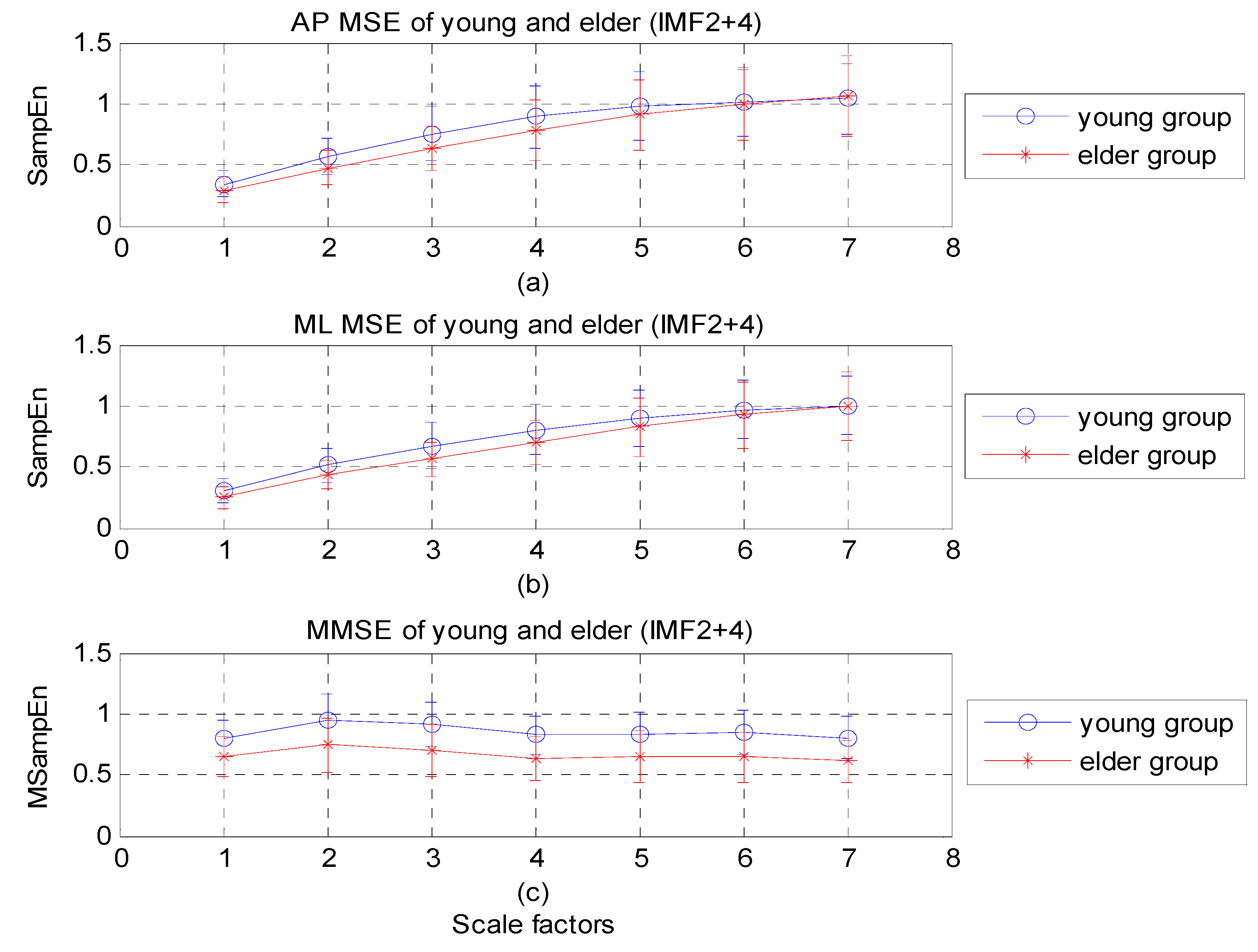
4.1. EMD-Enhanced MSE


| IMF | ML (x-direction) | AP (y-direction) | ||||
|---|---|---|---|---|---|---|
| Young | Elderly | p-value | Young | Elderly | p-value | |
| 2 | 2.73 ± 1.07 | 2.74 ± 1.30 | 0.972 | 4.07 ± 1.18 | 2.92 ± 1.03 | 0.002 |
| 3 | 3.05 ± 0.94 | 2.74 ± 0.68 | 0.240 | 3.44 ± 0.72 | 3.24 ± 0.90 | 0.444 |
| 4 | 2.92 ± 0.52 | 2.36 ± 0.49 | 0.001 | 2.81 ± 0.54 | 2.56 ± 0.61 | 0.180 |
| 5 (*) | 1.95 ± 0.48 | 1.61 ± 0.44 | 0.026 | 2.00 ± 0.49 | 1.66 ± 0.42 | 0.024 |
| 6 | 0.99 ± 0.43 | 0.84 ± 0.27 | 0.201 | 1.11 ± 0.36 | 0.79 ± 0.30 | 0.004 |
| 2+3 | 4.18 ± 1.43 | 3.93 ± 1.30 | 0.581 | 5.24 ± 1.15 | 3.93 ± 1.30 | 0.127 |
| 2+4 | 4.52 ± 1.16 | 4.07 ± 1.14 | 0.231 | 4.89 ± 1.34 | 4.48 ± 1.40 | 0.350 |
| 2+5 | 3.62 ± 0.93 | 3.73 ± 1.47 | 0.765 | 4.17 ± 1.26 | 3.80 ± 1.12 | 0.329 |
| 2+6 | 3.01 ± 1.32 | 3.54 ± 1.58 | 0.253 | 3.33 ± 0.99 | 3.22 ± 1.33 | 0.768 |
| 3+4 | 3.82 ± 0.88 | 3.16 ± 0.51 | 0.005 | 3.92 ± 0.87 | 3.50 ± 0.83 | 0.130 |
| 3+5 | 3.54 ± 0.92 | 3.04 ± 0.74 | 0.066 | 3.78 ± 0.80 | 3.26 ± 0.64 | 0.300 |
| 3+6 | 3.31 ± 1.23 | 2.85 ± 0.68 | 0.156 | 3.62 ± 0.72 | 3.02 ± 0.86 | 0.023 |
| 4+5(*) | 2.58 ± 0.45 | 2.22 ± 0.50 | 0.019 | 2.71 ± 0.41 | 2.21 ± 0.46 | 0.001 |
| 4+6 | 2.42 ± 0.69 | 2.14 ± 0.52 | 0.156 | 2.45 ± 0.52 | 2.03 ± 0.69 | 0.034 |
| 5+6 | 1.54 ± 0.63 | 1.27 ± 0.36 | 0.105 | 1.68 ± 0.39 | 1.29 ± 0.45 | 0.005 |
| 2+3+4 | 4.73 ± 1.12 | 4.13 ± 0.87 | 0.066 | 5.12 ± 1.33 | 4.69 ± 1.24 | 0.301 |
| 2+3+5 | 4.37 ± 1.15 | 4.06 ± 1.16 | 0.402 | 4.91 ± 1.11 | 4.37 ± 0.91 | 0.106 |
| 2+3+6 | 4.20 ± 1.51 | 3.92 ± 1.09 | 0.507 | 4.71 ± 0.98 | 4.21 ± 1.29 | 0.177 |
| 2+4+5 | 3.66 ± 0.83 | 3.63 ± 1.17 | 0.931 | 4.17 ± 1.11 | 3.77 ± 0.97 | 0.244 |
| 2+4+6 | 3.67 ± 1.20 | 3.66 ± 1.13 | 0.977 | 3.70 ± 0.92 | 3.54 ± 1.34 | 0.652 |
| 2+5+6 | 2.91 ± 1.05 | 3.26 ± 1.38 | 0.369 | 3.21 ± 0.83 | 3.05 ± 1.21 | 0.615 |
| 3+4+5(*) | 3.39 ± 0.66 | 2.96 ± 0.60 | 0.037 | 3.67 ± 0.70 | 3.19 ± 0.62 | 0.026 |
| 3+4+6 | 3.38 ± 0.89 | 2.92 ± 0.57 | 0.057 | 3.51 ± 0.68 | 3.06 ± 0.81 | 0.060 |
| 3+5+6 | 3.00 ± 0.90 | 2.73 ± 0.67 | 0.286 | 3.41 ± 0.72 | 2.82 ± 0.82 | 0.021 |
| 4+5+6 | 2.29 ± 0.61 | 2.07 ± 0.59 | 0.249 | 2.49 ± 0.37 | 1.99 ± 0.58 | 0.003 |
| 2+3+4+5 | 4.09 ± 0.84 | 3.94 ± 0.98 | 0.604 | 4.69 ± 1.12 | 4.25 ± 0.88 | 0.175 |
| 2+3+4+6 | 4.17 ± 1.15 | 3.90 ± 0.95 | 0.425 | 4.41 ± 0.98 | 4.05 ± 1.24 | 0.319 |
| 2+3+5+6 | 3.79 ± 1.17 | 3.68 ± 1.10 | 0.758 | 4.33 ± 0.93 | 3.85 ± 1.16 | 0.157 |
| 2+4+5+6 | 3.24 ± 0.94 | 3.39 ± 1.13 | 0.648 | 3.66 ± 0.82 | 3.67 ± 1.12 | 0.352 |
| 3+4+5+6 | 3.12 ± 0.71 | 2.77 ± 0.62 | 0.110 | 3.41 ± 0.56 | 2.90 ± 0.73 | 0.020 |
| 2+3+4+5+6 | 3.77 ± 0.90 | 3.71 ± 0.98 | 0.842 | 4.23 ± 0.93 | 3.89 ± 1.07 | 0.282 |
| IMF | ML (x-direction) | AP (y-direction) | ||||
|---|---|---|---|---|---|---|
| Before | After | p-value | Before | After | p-value | |
| 5 | 1.52 ± 0.33 | 1.56 ± 0.44 | 0.702 | 1.87 ± 0.51 | 1.90 ± 0.36 | 0.803 |
| 4+5 | 2.26 ± 0.41 | 2.18 ± 0.51 | 0.439 | 2.51 ± 0.53 | 2.58 ± 0.52 | 0.641 |
| 3+4+5 | 3.03 ± 0.40 | 2.98 ± 0.52 | 0.731 | 3.56 ± 0.85 | 3.64 ± 0.82 | 0.733 |
4.2. MEMD-Enhanced MMSE
| IMF | Young | Elderly | p-value |
|---|---|---|---|
| 2 | 4.07 ± 0.57 | 3.74 ± 0.68 | 0.117 |
| 3 | 4.18 ± 0.74 | 3.69 ± 1.04 | 0.095 |
| 4(*) | 4.57 ± 0.85 | 3.61 ± 1.00 | 0.002 |
| 5 | 4.23 ± 0.73 | 3.70 ± 0.94 | 0.053 |
| 6 | 4.10 ± 0.77 | 3.83 ± 0.64 | 0.237 |
| 2+3 | 4.82 ± 0.77 | 4.31 ± 1.16 | 0.114 |
| 2+4(*) | 5.18 ± 1.03 | 4.01 ± 1.18 | 0.002 |
| 2+5(*) | 4.63 ± 0.75 | 3.91 ± 1.08 | 0.019 |
| 2+6 | 4.30 ± 0.84 | 3.92 ± 0.61 | 0.111 |
| 3+4(*) | 5.26 ± 0.96 | 4.18 ± 1.04 | 0.002 |
| 3+5(*) | 5.13 ± 0.69 | 4.24 ± 1.16 | 0.006 |
| 3+6 | 4.77 ± 0.89 | 4.28 ± 0.62 | 0.051 |
| 4+5(*) | 5.08 ± 0.83 | 4.31 ± 1.06 | 0.015 |
| 4+6(*) | 5.13 ± 0.78 | 4.59 ± 0.70 | 0.026 |
| 5+6 | 4.26 ± 0.65 | 4.34 ± 0.62 | 0.687 |
| 2+3+4(*) | 5.59 ± 1.10 | 4.47 ± 1.18 | 0.003 |
| 2+3+5(*) | 5.41 ± 0.71 | 4.41 ± 1.24 | 0.004 |
| 2+3+6(*) | 4.92 ± 0.91 | 4.36 ± 0.61 | 0.029 |
| 2+4+5(*) | 5.31 ± 0.93 | 4.42 ± 1.12 | 0.010 |
| 2+4+6(*) | 5.28 ± 0.84 | 4.66 ± 0.69 | 0.015 |
| 2+5+6 | 4.38 ± 0.68 | 4.41 ± 0.64 | 0.864 |
| 3+4+5(*) | 5.54 ± 0.89 | 4.61 ± 1.15 | 0.007 |
| 3+4+6(*) | 5.51 ± 0.87 | 4.84 ± 0.75 | 0.014 |
| 3+5+6 | 4.60 ± 0.75 | 4.55 ± 0.68 | 0.828 |
| 4+5+6 | 4.88 ± 0.68 | 4.74 ± 0.77 | 0.552 |
| 2+3+4+5(*) | 5.75 ± 0.97 | 4.74 ± 1.24 | 0.007 |
| 2+3+4+6(*) | 5.61 ± 0.89 | 4.94 ± 0.74 | 0.013 |
| 2+3+5+6 | 4.62 ± 0.78 | 4.53 ± 0.68 | 0.707 |
| 2+4+5+6 | 4.97 ± 0.71 | 4.79 ± 0.80 | 0.457 |
| 3+4+5+6 | 5.15 ± 0.76 | 4.89 ± 0.82 | 0.308 |
| 2+3+4+5+6 | 5.28 ± 0.81 | 4.95 ± 0.84 | 0.227 |
| IMF | Before | After | p-value |
|---|---|---|---|
| 4 | 3.06 ± 1.13 | 3.74 ± 0.96 | 0.028 |
| 2+4 | 3.55 ± 1.35 | 4.32 ± 1.18 | 0.037 |
| 3+4 | 3.78 ± 1.38 | 4.64 ± 1.21 | 0.027 |
| 2+3+4 | 4.03 ± 1.47 | 4.93 ± 1.30 | 0.030 |
4.3. Comparison between EMD-Enhanced MSE and MEMD-Enhanced MMSE in Analysis of COP
| ID | MMSE | MSE | |||||||||||||
|---|---|---|---|---|---|---|---|---|---|---|---|---|---|---|---|
| ML&AP | ML (x-axis) | AP (y-axis) | |||||||||||||
| Before | After | Diff | Before | After | Diff | Before | After | Diff | |||||||
| 1 | 3.50 | 4.51 | 1.01 | 3.45 | 4.59 | 1.13 | 3.63 | 6.99 | 3.36 | ||||||
| 2 | 3.76 | 3.54 | −0.22 | 4.39 | 4.48 | 0.08 | 6.29 | 5.46 | −0.83 | ||||||
| 3 | 3.52 | 4.75 | 1.23 | 3.51 | 4.16 | 0.65 | 5.18 | 5.30 | 0.12 | ||||||
| 4 | 3.07 | 4.84 | 1.77 | 3.42 | 3.06 | −0.35 | 5.76 | 4.77 | −1.00 | ||||||
| 5 | 5.57 | 4.66 | −0.91 | 2.75 | 4.97 | 2.22 | 5.15 | 5.95 | 0.80 | ||||||
| 6 | 2.95 | 5.49 | 2.55 | 3.69 | 2.08 | −1.61 | 3.51 | 6.35 | 2.84 | ||||||
| 7 | 4.42 | 5.51 | 1.09 | 5.30 | 3.87 | −1.44 | 6.48 | 5.16 | −1.32 | ||||||
| 8 | 2.11 | 5.43 | 3.33 | 4.13 | 4.64 | 0.51 | 6.60 | 6.57 | −0.02 | ||||||
| 9 | 5.70 | 5.51 | −0.19 | 4.37 | 5.75 | 1.38 | 6.10 | 6.54 | 0.43 | ||||||
| 10 | 2.62 | 1.88 | −0.75 | 3.94 | 4.32 | 0.38 | 5.24 | 4.26 | −0.97 | ||||||
| 11 | 1.05 | 6.14 | 5.10 | 3.07 | 4.51 | 1.44 | 1.37 | 6.38 | 5.02 | ||||||
| 12 | 2.68 | 5.97 | 3.29 | 3.35 | 3.61 | 0.26 | 5.23 | 4.67 | −0.57 | ||||||
| 13 | 4.34 | 4.25 | −0.09 | 4.14 | 2.58 | −1.57 | 5.97 | 6.00 | 0.03 | ||||||
| 14 | 5.51 | 5.70 | 0.19 | 5.75 | 4.37 | −1.38 | 6.54 | 6.10 | −0.43 | ||||||
| 15 | 3.02 | 5.97 | 2.95 | 3.16 | 4.83 | 1.67 | 4.01 | 6.48 | 2.47 | ||||||
| 16 | 3.98 | 3.50 | −0.48 | 4.86 | 3.71 | −1.15 | 5.50 | 5.26 | −0.24 | ||||||
| 17 | 5.21 | 5.37 | 0.16 | 3.45 | 3.68 | 0.22 | 5.58 | 5.30 | −0.28 | ||||||
| 18 | 5.68 | 0.96 | −4.71 | 6.94 | 4.16 | −2.78 | 7.00 | 0.56 | −6.44 | ||||||
| 19 | 5.82 | 5.50 | −0.32 | 3.11 | 3.43 | 0.33 | 5.92 | 4.40 | −1.53 | ||||||
| 20 | 2.14 | 5.35 | 3.20 | 3.66 | 3.78 | 0.12 | 3.50 | 4.79 | 1.29 | ||||||
| 21 | 5.67 | 5.40 | −0.27 | 4.63 | 3.35 | −1.28 | 7.41 | 6.39 | −1.02 | ||||||
| 22 | 6.24 | 5.48 | −0.76 | 4.08 | 4.12 | 0.03 | 4.92 | 4.10 | −0.82 | ||||||
| 23 | 6.42 | 6.64 | 0.22 | 5.81 | 6.34 | 0.53 | 6.91 | 8.17 | 1.25 | ||||||
| 24 | 3.76 | 4.49 | 0.73 | 3.51 | 3.45 | −0.06 | 4.80 | 4.38 | −0.43 | ||||||
| 25 | 3.02 | 6.55 | 3.53 | 4.01 | 3.33 | −0.69 | 5.55 | 5.38 | −0.16 | ||||||
| 26 | 2.86 | 4.74 | 1.88 | 3.84 | 3.85 | 0.02 | 6.31 | 5.34 | −0.96 | ||||||
| Mean ± SD | 4.03 ± 1.47 | 4.93 ± 1.30 | 0.91 ± 2.00 | 4.09 ± 0.98 | 4.04 ± 0.90 | −0.05 ± 1.18 | 5.40 ± 1.34 | 5.43 ± 1.38 | 0.02 ± 2.06 | ||||||
| p−value | 0.03 | 0.827 | 0.955 | ||||||||||||
| Improve | 16/26 = 61.5% | 8/26 = 30.8% | |||||||||||||
5. Discussion
6. Conclusions
Acknowledgments
References
- Roudsari, B.S.; Ebel, B.E.; Corso, P.S.; Molinari, N.M.; Koepsell, T.D. The acute medical care costs of fall-related injuries among the U.S older adults. J. Care Injured. 2005, 36, 1316–1322. [Google Scholar] [CrossRef] [PubMed]
- Gefen, A. Simulations of foot stability during gait characteristic of ankle dorsiflexor weakness in the elderly. IEEE Trans. Neur. Sys. Reh. 2001, 9, 333–337. [Google Scholar] [CrossRef] [PubMed]
- Jiang, S.S.; Zhang, B.F.; Wei, D.M. The elderly fall risk assessment and prediction based on gait analysis. In Proceedings of 2011 IEEE 11th International Conference on Computer and Information Technology (CIT), Pafos, Cyprus, 31 August–2 September 2011; pp. 176–180.
- McDonnell, M.D.; Stocks, N.G.; Pearce, C.E.M.; Derek, A. Stochastic Resonance: from Supra Threshold Stochastic Resonance to Stochastic Signal Quantization, 1st ed.; Cambridge University Press: Cambridge, UK, 2008; pp. 6–20. [Google Scholar]
- Moss, F.; Ward, L.M.; Sannita, W.G. Stochastic resonance and sensory information processing: a tutorial and review of application. Clin. Neurophysiol. 2004, 115, 267–281. [Google Scholar] [CrossRef] [PubMed]
- Liu, W.; Lipsitz, L.A.; Montero-Odasso, M.; Bean, J.; Kerrigan, D.C.; Collins, J.J. Noise-enhanced vibrotactile sensitivity in older adults, patients with stroke, and patients with diabetic neuropathy. Arch. Phys. Med. Rehabil. 2002, 83, 171–176. [Google Scholar] [CrossRef] [PubMed]
- Novak, P.; Novak, V. Effect of step-synchronized vibration stimulation of soles on gait in Parkinson’s disease: a pilot study. J. Neuroeng. Rehabil. 2006, 3, 9–15. [Google Scholar] [CrossRef] [PubMed]
- Pajala, S.; Era, P.; Koskenvuo, M.; Kaprio, J.; Törmäkangas, T.; Rantanen, T. Force platform balance measures as predictors of indoor and outdoor falls in community-dwelling women aged 63–76 years. J. Gerontol. A 2008, 63, 171–178. [Google Scholar] [CrossRef]
- Costa, M.; Priplata, A.A.; Lipsitz, L.A.; Wu, Z.; Huang, N.E.; Goldberger, A.L.; and Peng, C.-K. Noise and poise: Enhancement of postural complexity in the elderly with a stochastic-resonance-based therapy. Europhys. Lett. 2007, 68008. [Google Scholar] [CrossRef] [PubMed]
- Chen, S.J.; Gielo-Perczak, K. Effect of impeded medial longitudinal arch drop on vertical ground reaction force and center of pressure during static loading. Foot Ankle Int. 2011, 32, 77–84. [Google Scholar] [CrossRef] [PubMed]
- Van Wegan, E.E.H.; Van Emmerik, R.E.A.; Riccio, G.E. Postural orientation: Age-related changes in variability and time-to-boundary. Hum. Movement Sci. 2002, 21, 61–68. [Google Scholar] [CrossRef]
- Lai, C.-L.; Tseng, S.-Y.; Huang, C.-H.; Pei, C.; Chi, W.-M.; Hsu, L.-C.; Sun, T.-L. Fun and accurate static balance training to enhance fall prevention ability of aged adults: A preliminary study. Hum. Factors Ergonom. Manuf. Serv. Ind. 2012. [CrossRef]
- Jiang, B.C.; Yang, W.-H.; Shieh, J.-S.; Fan, S.-Z.; Peng, C.-K. Entropy-based method for COP data analysis. Theor. Issues Ergonomics Sci. 2012. [CrossRef]
- Costa, M.; Goldberger, A.L.; Peng, C.-K. Multiscale entropy analysis of biological signals. Phys. Rev. E. 2005. [CrossRef]
- Sarkar, A.; Barat, P. Multiscale entropy analysis: A new method to detect determinism in a time series. Entropy 2006, 8, 1–9. [Google Scholar]
- Huang, N.E.; Shen, Z.; Long, S.R.; Wu, M.C.; Shih, H.H.; Zheng, Q.; Yen, N.C.; Tung, C.C.; Liu, H.H. The empirical mode decomposition and Hilbert spectrum for nonlinear and nonstationary time series analysis. Proc. R. Soc. Lond. A 1998, 454, 903–995. [Google Scholar] [CrossRef]
- Rehman, N.; Mandic, D.P. Multivariate empirical mode decomposition. Proc. R. Soc. A 2010, 466, 1291–1302. [Google Scholar] [CrossRef]
- Ahmed, M.U.; Mandic, D.P. Multivariate multiscale entropy: A tool for complexity analysis of multichannel data. Phys. Review E. 2011, 061918. [Google Scholar] [CrossRef]
- Morabito, F.C.; Labate, D.; La Foresta, F.; Bramanti, A.; Morabito, G.; Palamara, I. Multivariate Multi-Scale Permutation Entropy for Complexity Analysis of Alzheimer’s Disease EEG. Entropy 2012, 14, 1186–1202. [Google Scholar] [CrossRef]
- Rehman, N.; Mandic, D.P. Filter bank property of multivariate empirical mode decomposition. IEEE Trans. Signal Proc. 2010, 59, 2421–2426. [Google Scholar] [CrossRef]
- Zhou, X.; Yang, T.; Zou, H.-L.; Zhao, H. Multivariate empirical mode decomposition approach for adaptive denoising of fringe patterns. Opt. Lett. 2012, 37, 1904–1906. [Google Scholar] [CrossRef] [PubMed]
- Costa, M.; Goldberger, A.L.; Peng, C.K. Multiscale entropy analysis of complex physiologic time series. Phys. Rev. Lett. 2002. [CrossRef]
- Costa, M.; Peng, C.-K.; Goldberger, A.L.; Hausdorff, J.M. Multiscale entropy analysis of human gait dynamics. Physica A 2003, 330, 53–60. [Google Scholar] [CrossRef]
- Thuraisingham, R.A.; Gottwald, G.A. On multiscale entropy analysis for physiological data. Physica A 2006, 366, 323–332. [Google Scholar] [CrossRef]
- Richman, J.; Moorman, J. Physiological time series analysis using approximate entropy and sample entropy. Am. J. Physiol. 2000, 278, H2039–H2049. [Google Scholar]
- Yeh, J.R.; Shieh, J.S.; Huang, N.E. Complementary ensemble empirical mode decomposition: A novel noise enhanced data analysis method. Adv. Adapt. Data Anal. 2010, 02, 135–156. [Google Scholar] [CrossRef]
- Yeh, J.R.; Lin, T.-Y.; Chen, Y.; Sun, W.-Z.; Abbod, M.F.; Shieh, J.-S. Investigating properties of the cardiovascular system using innovative analysis algorithms based on ensemble empirical mode decomposition. Comp. Math. Method Med. 2012, 2012, 943431. [Google Scholar] [CrossRef] [PubMed]
- Hu, K.; Peng, C.K.; Czosnyka, M.; Zhao, P.; Novak, V. Nonlinear assessment of cerebral autoregulation from spontaneous blood pressure and cerebral blood flow fluctuations. Cardiovasc. Eng. 2008, 8, 60–71. [Google Scholar] [CrossRef] [PubMed]
- Hu, M; Liang, H.L. Adaptive multiscale entropy analysis of multivariate neural data. IEEE Trans. Biomed. Eng. 2012, 59, 12–15. [Google Scholar]
- Liu, Q.; Wei, Q.; Fan, S.-Z.; Lu, C.-W.; Lin, T.-Y.; Abbod, M.F.; Shieh, J.-S. Adaptive computation of multiscale entropy and its application in EEG signals for monitoring depth of anesthesia during surgery. Entropy 2012, 14, 978–992. [Google Scholar] [CrossRef]
- Chen, D.; Li, D.; Xiong, M.Z.; Bao, H.; Li, X.L. GPGPU-aided ensemble empirical-mode decomposition for EEG analysis during anesthesia. IEEE Trans. Inf. Technol. B. 2010, 14, 1417–1427. [Google Scholar] [CrossRef] [PubMed]
© 2012 by the authors; licensee MDPI, Basel, Switzerland. This article is an open access article distributed under the terms and conditions of the Creative Commons Attribution license (http://creativecommons.org/licenses/by/3.0/).
Share and Cite
Wei, Q.; Liu, D.-H.; Wang, K.-H.; Liu, Q.; Abbod, M.F.; Jiang, B.C.; Chen, K.-P.; Wu, C.; Shieh, J.-S. Multivariate Multiscale Entropy Applied to Center of Pressure Signals Analysis: An Effect of Vibration Stimulation of Shoes. Entropy 2012, 14, 2157-2172. https://doi.org/10.3390/e14112157
Wei Q, Liu D-H, Wang K-H, Liu Q, Abbod MF, Jiang BC, Chen K-P, Wu C, Shieh J-S. Multivariate Multiscale Entropy Applied to Center of Pressure Signals Analysis: An Effect of Vibration Stimulation of Shoes. Entropy. 2012; 14(11):2157-2172. https://doi.org/10.3390/e14112157
Chicago/Turabian StyleWei, Qin, Dong-Hai Liu, Kai-Hong Wang, Quan Liu, Maysam F. Abbod, Bernard C. Jiang, Ku-Ping Chen, Chuan Wu, and Jiann-Shing Shieh. 2012. "Multivariate Multiscale Entropy Applied to Center of Pressure Signals Analysis: An Effect of Vibration Stimulation of Shoes" Entropy 14, no. 11: 2157-2172. https://doi.org/10.3390/e14112157
APA StyleWei, Q., Liu, D.-H., Wang, K.-H., Liu, Q., Abbod, M. F., Jiang, B. C., Chen, K.-P., Wu, C., & Shieh, J.-S. (2012). Multivariate Multiscale Entropy Applied to Center of Pressure Signals Analysis: An Effect of Vibration Stimulation of Shoes. Entropy, 14(11), 2157-2172. https://doi.org/10.3390/e14112157